Strömgren photometry of Galactic Globular Clusters. II Metallicity distribution of red giants in $\omega$ Centauri.

Abstract

We present new intermediate-band Strömgren photometry based on more than 300 $u,v,b,y$ images of the Galactic globular cluster $\omega$ Cen. Optical data were supplemented with new multiband near-infrared (NIR) photometry (350 $J,H,K_{s}$ images). The final optical-NIR catalog covers a region of more than $20\times 20$ arcmin squared across the cluster center. We use different optical-NIR color-color planes together with proper motion data available in the literature to identify candidate cluster red giant (RG) stars. By adopting different Strömgren metallicity indices we estimate the photometric metallicity for $\approx 4,000$ RGs, the largest sample ever collected. The metallicity distributions show multiple peaks ($\hbox{\rm[Fe/H]}_{phot}=$ $-1.73\pm 0.08$, $-1.29\pm 0.03$, $-1.05\pm 0.02$, $-0.80\pm 0.04$, $-0.42\pm 0.12$ and $-0.07\pm 0.08$ dex) and a sharp cut-off in the metal-poor tail ($\hbox{\rm[Fe/H]}_{phot}\lesssim-2$ dex) that agree quite well with spectroscopic measurements. We identify four distinct sub-populations, namely metal-poor (MP, $\hbox{\rm[Fe/H]}\leq-1.49$), metal-intermediate (MI, $-1.49<\hbox{\rm[Fe/H]}\leq-0.93$), metal-rich (MR, $-0.95<\hbox{\rm[Fe/H]}\leq-0.15$) and solar metallicity (SM, $\hbox{\rm[Fe/H]}\approx 0$). The last group includes only a small fraction of stars ($\sim\;8\pm 5$%) and should be confirmed spectroscopically. Moreover, using the difference in metallicity based on different photometric indices, we find that the $19\pm 1$% of RGs are candidate CN-strong stars. This fraction agrees quite well with recent spectroscopic estimates and could imply a large fraction of binary stars. The Strömgren metallicity indices display a robust correlation with $\alpha$-elements ([Ca+Si/H]) when moving from the metal-intermediate to the metal-rich regime ($\hbox{\rm[Fe/H]}\gtrsim-1.7$ dex).

1. Introduction

The Galactic Globular Cluster (GGC) $\omega$ Cen (NGC 5139) is currently the target of significant observational efforts covering the whole wavelength spectrum. This huge star cluster, the most massive known in our Galaxy (2.5 $\times 10^{6}$ $M_{\odot}\,$, van de Ven et al. 2006) hosts at least three separate stellar populations with a large undisputed spread in metallicity (Norris & Da Costa 1995; hereinafter ND95; Norris et al. 1996, hereinafter N96; Suntzeff & Kraft 1996, hereinafter SK96; Smith et al. 2000, hereinafter SM00; Kayser et al. 2006, hereinafter KA06; Villanova et al. 2007). The most relevant morphological and structural parameters of $\omega$ Cen are summarized in Table 1.

The unusual spread in color of the red giant branch (RGB) in $\omega$ Cen was revealed for the first time by Dickens & Woolley (1967) using photographic photometry by Woolley (1966), and later verified by Cannon & Stobie (1973) using photoelectric photometry. The width in color of the RGB was interpreted as an indication of an intrinsic spread in chemical abundance, as subsequently confirmed by spectroscopic data (Freemann & Rodgers 1975). Moreover, recent photometric surveys by Lee et al. (1999), Pancino et al. (2000, hereinafter PA00), Rey et al. (2004) and Sollima et al. (2005a, hereinafter S05a), disclosed the discrete nature of the $\omega$ Cen RGBs.

More recent spectroscopic studies of red-giant (RG) stars have refined our knowledge of the intrinsic spread in heavy elements in $\omega$ Cen (ND95; N96; SK96). In particular, the low-resolution study of $\approx$ 500 RGs performed by N96 and by SK96, based on the Ca $H$, $K$ lines, and on the infrared CaII triplet (CaT), provided a metallicity distribution with a dominant peak located at [Fe/H] $\approx$–1.6, a secondary peak at [Fe/H] $\approx$–1.2, and a long, asymmetric tail extending toward higher metallicities ([Fe/H] $\approx$–0.5). This distribution agrees quite well with the metallicity distributions obtained by Hilker & Richtler (2000, hereinafter HR00, $\sim$1,500 RGs) and by Hughes et al. (2004, $\sim$2500 MS, SGB, RG) using the Strömgren $(m_{0},\hbox{\it b--y\/})$ metallicity diagnostic and by S05a using the $(B-V)$ color of $\sim$1,400 RG stars.

Moreover, $\alpha$-element abundance differences have been detected among $\omega$ Cen RGs. They show typical overabundances ($[\alpha/Fe]\sim 0.3-0.4$) up to iron abundances of [Fe/H] $\sim$–0.8 (SM00; Cunha et al. 2002; Vanture et al. 2002) and evidence of a decrease in the overabundance to $[\alpha/Fe]\approx 0.1$ in the more metal-rich regime (Pancino et al. 2002, hereinafter PA02; Gratton, Sneden, & Carretta 2004). The large range of heavy element abundances observed among cluster RGs was also detected among sub-giant branch (SGB) and main sequence turn-off (MSTO) stars. In particular, Hilker et al. (2004, hereinafter H04) and KA06, based on medium-resolution spectra of more than 400 SGB and MSTO stars, found a metallicity distribution with three well defined peaks around [Fe/H] = –1.7, –1.5 and –1.2, together with a handful of metal-rich stars with $\hbox{\rm[Fe/H]}\,\sim\,$–0.8. Furthermore, metal-rich stars seem to be CN-enriched, while metal-poor stars show high CH abundances (KA06). Using the infrared CaT of 250 SGB stars, Sollima et al. (2005b, hereinafter S05b) found a similar metallicity distribution with four peaks located at [Fe/H] =–1.7, –1.3, –1.0, and –0.6 dex. The recent metallicity distribution based on low-resolution spectroscopy of 442 MSTO and SGB stars by Stanford et al. (2006a) confirmed the occurrence of a sharp rise at low metallicities, $\hbox{\rm[Fe/H]}<$ –1.7, and the presence of a metal-rich tail up to $\hbox{\rm[Fe/H]}\,\approx\,$–0.6 dex. Moreover, Stanford et al. (2007), using the same spectra, showed that $\sim$16–17% of the SGB stars are enhanced in either C or N . In order to explain this interesting evidence they suggested that these enhancements might be due to primordial chemical enrichment either by low (1–3 M/$M_{\odot}\,$) to intermediate (3–8 M/$M_{\odot}\,$) mass AGB stars, or by massive rotating stars (Maeder & Meynet 2006).

This is the second paper of a series devoted to Strömgren photometry of GGCs. In the first paper we provided new empirical and semi-empirical calibrations of the metallicity index $m_{1}=(\hbox{\it v--b\/})-(\hbox{\it b--y\/})$ based on cluster RG stars and on new sets of semi-empirical and theoretical color-temperature relations (Calamida et al. 2007, hereinafter CA07).

The structure of the paper is as follows. In §2 we discuss in detail the multiband Strömgren ($u,v,b,y$) and near-infrared (NIR, $J,H,K_{s}$ ) images we collected for this experiment. In §3 and §4 we lay out the data reduction techniques and the calibration strategies adopted for the different data sets. Section 5 deals with the selection criteria adopted to identify candidate field and cluster RG stars using both optical and NIR photometry. In §6 we present a new calibration of the Strömgren $m_{1}$ metallicity index based on the b–y color and compare the new relation with similar relations available in the literature. In §7 we discuss the comparison between spectroscopic and photometric metallicities of $\omega$ Cen RG stars based on different Metallicity Index Color (MIC) relations and different calibrations (empirical, semi-empirical). In this section we also address the impact that CN-strong stars have on photometric metallicity estimates. Section 8 deals with metal abundance distributions—in particular, we discuss the occurrence of different metallicity regimes—while abundance anomalies ($C,N$, $\alpha$–elements) are discussed in §9. Finally, in §10 we summarize the results of this investigation and briefly outline possible future extensions of this medium-band photometric experiment.

2. Observations

2.1. Strömgren data

A set of 110 uvby Strömgren images centered on the cluster $\omega$ Cen was collected by one of us (LF) over 11 nights between 1999 March 27 to April 9, with the 1.54m Danish Telescope (ESO, La Silla). Weather conditions were good, typically with humidity from 40–60%, conditions frequently photometric, and seeing ranging from 1^′′.3 for the $y$ band to 2^′′.3 for the $u$ band. On clear photometric nights, $\omega$ Cen was observed with exposure times of 1200s, 480s, 240s, 120s for the uvby bands, while on less photometric nights, we used exposure times of 2000s, 900s, 600s and 450s. The CCD camera was a 2048$\times$2048 pixel Ford-Loral CCD, with a pixel scale of 0^′′.39 and a field of view of 13^′.7$\times$13^′.7. The CCD has two amplifiers, A and B, and we used A in high-gain mode for our observations. The gain and the readout noise (RON) of the CCD were measured to be $1.3\pm 0.01$ e^-/ADU and $8.25\pm 0.1$ e^-, respectively.

This data set has been supplemented with 30 uvby images of the SW quadrant of $\omega$ Cen collected by one of us (FG) during four nights in April 1999 and two nights in June 1999 with the Danish Telescope. During these nights a set of 112 HD standard stars was observed in the uvby bands. These were selected from the catalogs of photometric standards by Schuster & Nissen (1988, hereinafter SN88) and by Olsen (1993, hereinafter O93). Table 2 and Table 3 give the log of these observations together with the seeing conditions.

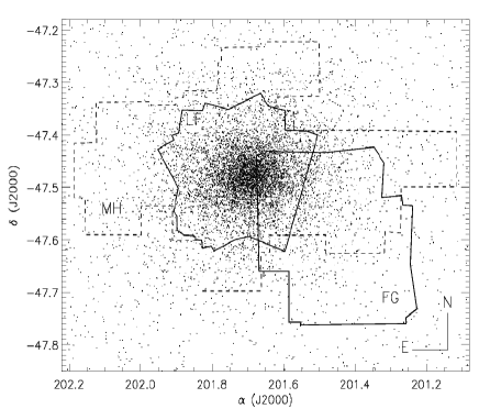
Figure 1.— The coverage of the three Strömgren data sets collected with the 1.54m Danish Telescope – L. Freyhammer (LF) central field, F. Grundahl (FG) SW fields, and M. Hilker (MH) field, superimposed to $\omega$ Cen. The background is a composite reference image of $\omega$ Cen based on randomly selected subsamples of stars from the Two Micron All Sky Survey (2MASS) and the van Leuwen et al. (2000) catalog.

Together with the aforementioned images we also acquired 210 vby images collected with the same telescope by two of us (MH, TR) in two observing runs (1993 and 1995, see Hilker 2000, hereinafter H00; HR00). The CCD used for these observations was a Tektronix 1024$\times$1024 chip, with a pixel scale of 0^′′.50 and a field of view of 6^′.3$\times$6^′.3. The log of this data set is given in Table 4 and specifics concerning the 33 fields used in this investigation are given in Table 2. To obtain a homogeneous photometric catalog, these frames were reanalyzed adopting the same procedure as was applied to the two other data sets. Fig. 1 shows the location of the three different data sets across the cluster area.

2.2. Near-Infrared data

Near-Infrared $J$, $H$, and $K_{s}$-band images of $\omega$ Cen were collected in two different runs—2001 February 5, 7, and 2002 February 2, 3, 24, 25—with the NIR camera SOFI at the NTT (ESO, La Silla). SOFI can operate at low and high spatial resolution. In the former case the pixel scale is 0^′′.292 and the field of view (FoV) is 4^′.94$\times$4^′.94, while in the latter the pixel scale is 0^′′.145 and the FoV is 2^′.47$\times$2^′.47. We observed three different fields at low resolution: field $A$ (36$J$, 55$Ks$) is located at the cluster center, field C (33$J$, 55$Ks$) is located $\sim 10$^′.5 NW of the center, and field $D$ (12$J$, 20$Ks$) is located $\sim 10$^′.7 SW of the center (see Table 5 and Fig. 2). The observing time was split between target observations on $\omega$ Cen and reference sky observations. For each pointing we acquired a set of $J$ (Detector Integration Time [DIT]=3s, Number of DIT [NDIT]=1) and $K_{s}$ (DIT=3s, NDIT=4) images. To supplement these data we retrieved from the ESO archive a mosaic of nine pointings (11$J$, 11$K_{s}$; Sollima et al. 2004) which covers an area of $\sim 13$^′$\times 13$^′across the cluster center. These images were collected on 2000 January 12, 13, using the same equipment in low-resolution mode.

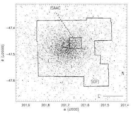
Figure 2.— Same as Fig. 1, but for a narrower cluster region showing the coverage of the two NIR data sets collected with SOFI@NTT and with ISAAC@VLT.

Moreover, we also retrieved from the ESO archive two more data sets collected during the nights 2004 June 3, 4 and 2005 April 2. These data sample three different positions: field $\alpha$ (15$J$, low resolution) located at the cluster center; field $\beta$ (15$J$, low resolution) located $\sim 5$^′ NW of the center; and field $\gamma$ located $\sim 5$^′ SE of the center. This last field was observed both at low ($\gamma_{1}$, 12$J$,12$H$,12$Ks$) and high ($\gamma_{2}$, 24$Ks$) spatial resolution.

The above data were further supplemented with a set of NIR images from the NIR camera ISAAC at the VLT (ESO, Paranal). Its pixel scale is 0^′′.145 and the FoV is 2^′.5$\times$2^′.5. The images were collected using two narrow-band filters centered on $\lambda=1.21\,\mu$m ($\Delta\lambda=0.018\,\mu$m; 8 images) and $\lambda=2.19\,\mu$m ($\Delta\lambda=0.03\,\mu$m; 24 images). We adopted the same $DIT$ of 6 sec, but $NDIT=13$ and 11 for the $NB\_1.21$ band and the $NB\_2.19$ band, respectively. The log of the entire NIR data set is given in Table 6, and the area covered by the different SOFI and ISAAC fields is shown in Fig. 2.

3. Data reduction

3.1. Strömgren data

Flat fields for the central LF field (see Table 2 and Fig. 1) were collected for the different filters and CCD settings at dusk and at dawn. The Danish Faint Object Spectrograph and Camera (DFOSC) was mounted with its File and Shutter Unit (FASU) on the telescope instrument adaptor. The 90 mm Strömgren filters were installed in the FASU. The main DFOSC instrument with the CCD camera can rotate with respect to the FASU around the optical axis, so to average out background gradients in the flat-fields—typically introduced by scattered light in the telescope and in the instrument due to inadequate baffling—we introduced offsets of 90 degrees between flat fields in the same bandpass. Because DFOSC is a focal-reducer instrument, low-level multiple reflections in the optics are known to cause effects such as sky concentration (Andersen et al. 1999). The science frames were similarly obtained with rotation offsets. For each science image a 2D bias frame was subtracted, then they were scaled in level according to prescan and overscan areas, and flat-fielded using standard IRAF tasks based on nightly averaged calibration images. The 90 mm filters turned out to be affected by the artifact known as ’filter ghosts’. The ghosts are located on the CCD images $\sim 20$ pixels leftward of saturated stars and typically have the shape of a flattened doughnut or a fan. The orientation of the ghost star may slightly change across the CCD field, but on average it is quite constant. The separation between the saturated star and its ghost is also rather constant. The orientation of the ghosts in the CCD images collected with different orientations is rotated by the same angle. This evidence indicates that the ghost is not caused by double reflected light between the filter and the CCD camera, but must occur in the filter itself. A similar effect was found by O’Connor et al. (1998) in optical images collected with the MOMI CCD camera available at the Nordic Optical Telescope (NOT, La Palma), and also in HST images collected with the WFPC2 (Krist 1995). The overall effect on our images is of the order of 0.4–1.1% in flux in $b,y$-band images and smaller in $u,v$-band images. This means that this effect is smaller than the typical photometric accuracy along the RGB. However to avoid spurious effects in the PSF photometry, we chose no PSF stars located in the neighborhood of saturated stars.

Raw images of the FG data set (see Table 2 and Fig. 1) were pre-processed using tasks available in the IRAF data-analysis environment for bias subtraction and flat-fielding. To flat-field these data we adopted median sky flats collected during the observing nights. The reader interested in the details of pre-reduction strategy adopted for the MH images is referred to H00.

The photometry was performed using DAOPHOT IV/ALLSTAR and ALLFRAME (Stetson 1987; 1991; 1994). We first estimated a point-spread function (PSF) for each frame from $\approx 100$ bright, isolated stars, uniformly distributed on the chip. We assumed a spatially varying Moffat function for the PSF. We performed preliminary PSF photometry on each image with the task ALLSTAR. Then we used the task DAOMATCH/DAOMASTER (Stetson 1994) to merge the individual detection lists from the 328 images of the three different data sets into a single global star catalog referred to a common coordinate system. Twelve images were neglected, due to either bad seeing or poor image quality. As a reference catalog we adopted $B,V,I$-band photometry for $\approx$ 270,000 stars of $\omega$ Cen (Stetson 2000). These stars are distributed over a field of about 28^′$\times$28^′ centered on the cluster and have been selected for photometric precision $\sigma_{B,V,I}\leq$ 0.03 mag. We then performed simultaneous PSF-fitting photometry over the entire data set with the task ALLFRAME. Aperture corrections were determined for each frame and applied to the individual stellar magnitudes before the weighted mean magnitudes were determined (Calamida et al. 2008b). The final merged star catalog includes $\approx 2\times 10^{5}$ stars having measurements in at least two bands and covers a field of about 23^′$\times$23^′ centered on $\omega$ Cen.

3.2. Near-Infrared data

The reduction process for the NIR data was the same as for the optical data. The pre-reduction was performed using standard IRAF procedures, and initial photometry for individual images was performed with DAOPHOT/ALLSTAR. Then the individual detection lists were merged into a single star catalog and a new photometric reduction was performed with ALLFRAME. To improve the photometric accuracy we did not stack individual images, and the spatially varying PSFs were derived from at least 50 bright, isolated stars uniformly distributed across each image.

4. Photometric calibration

4.1. Strömgren data

Figure 3.— Calibration curves for the reference night June 6.

Standard stars for the Strömgren photometry were selected from the lists of Henry Draper stars published by SN88 and O93; these were observed during four nights in April 1999 and two nights in June 1999 (see Grundahl, Stetson, & Andersen 2002 for more details). Table 7 and 8 show the observation logs for these stars. We applied the same pre-reduction strategy and performed aperture photometry on the standard frames, ending up with a list of $\approx$ 20 HD stars per night. Extinction coefficients were estimated from observations of HD stars obtained at different airmass values (see Table 9). Coefficients estimated for three out of the four nights in April are mutually consistent, but the values obtained for June 6 are slightly larger (see Table 10). We estimated independent color transformations for each night and thus obtained a set of six calibration curves. These agree quite well with each other and we finally selected the best photometric night (June 6) to perform an absolute calibration of the scientific frames collected during this night. The calibration curves for the reference night are (see also Fig. 3):

$u=u_{i}-(3.012\pm 0.015)+(0.127\pm 0.010)\times(u_{i}-b_{i})$,

$v=v_{i}-(2.820\pm 0.008)+(0.002\pm 0.016)\times(v_{i}-b_{i})$,

$b=b_{i}-(2.488\pm 0.012)$,

$y=y_{i}-(2.736\pm 0.010)$.

where $i$ stands for the $instrumental$ magnitude.

On the basis of this calibration we defined a set of secondary standard stars, by selecting both according to photometric precision ($\sigma_{u,v,b,y}\leq$ 0.05 mag) and according to the ”separation index” ($sep_{v}$ > 5) in the calibrated star catalog of the reference night. We ended up with a sample of $\sim$5000 stars having measurements in all the Strömgren bands. We extended the photometric system of the reference data to each overlapping field by an iterative procedure.

In estimating the mean calibrated magnitudes, we neglected the $b$ and $y$ frames of the LF data set because the estimate of the aperture correction was hampered by the severe stellar crowding. For two pointings of the MH data set, namely fields $q$ and $r$ (see Fig. 1 of H00), the number of local standards was too small to provide a robust estimate of the calibration curves and they have not been included in the final catalog.

Figure 4.— Comparison between the $m_{1}$ index of $\omega$ Cen stars measured by HR00 and current photometry.

A slightly different approach was applied to the MH 1993 data. This data set included many non-photometric nights (see Table 4), and there were only a few secondary standards in this region of $\omega$ Cen. Therefore, the estimate of the relative zero-points between the different frames was difficult. Thus we used the final calibrated star catalog based on the other observations as a new set of local standard stars to individually calibrate each frame of the 1993 data set. However, fields 3, 4 and 8 (see Fig. 1 of HR00) were not included because the number of secondary standards was still too small in this cluster region. The typical accuracy of the absolute zero-point calibration is $\sim$ 0.02 mag for the $u,v$-band data and $\sim$ 0.015 mag for the $b,y$-band data.

We compared our calibration with the absolute calibrations provided by Richter et al. (1999), by Mukherjee et al. (1992) and by Hughes & Wallerstein (2000). Fig. 4 shows the comparison between the $m_{1}$ index based on the current photometry and the $m_{1}$ index based on the Richter et al. photometry. The mean difference is $\Delta(m_{1})\sim$ 0.00 with a dispersion of $\sigma\sim$ 0.03 mag. The mean differences between our and the other two studies are $\Delta(m_{1})\sim$ 0.01, with $\sigma\sim$ 0.06 based on 139 stars in common with the Mukherjee et al. catalog, and $\Delta(m_{1})\sim$ -0.02, with $\sigma\sim$ 0.05, based on 228 stars in common with the Hughes & Wallerstein catalog.

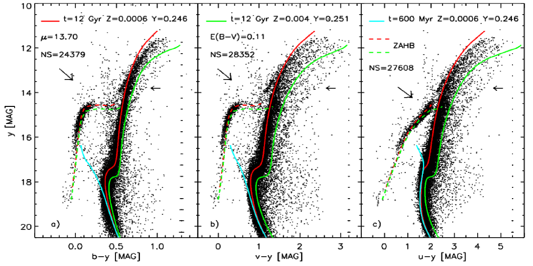
Figure 5.— From left to right a) $y$, b–y; b) $y$, v–y; c) $y$, u–y  Strömgren CMDs of $\omega$ Cen. Stars were selected according to photometric accuracy—$\sigma_{u,v}\leq$ 0.05 mag, $\sigma_{b,y}\leq$0.03 mag—and separation—$sep_{v}\geq 2$, $sep_{b,y}\geq 3$. The red and the green solid lines represent two cluster isochrones at fixed age ($t=12$ Gyr) and different chemical compositions (see labeled values). The dashed lines show two ZAHBs for the same chemical compositions and a progenitor mass of 0.8 $M/M_{\odot}$. The turquoise solid line shows a young ($t=600$ Myr), metal-poor cluster isochrone. The true distance modulus ($\mu$) and the reddening adopted to overplot the theoretical predictions are also labeled. Error bars plotted on the right side show the intrinsic photometric uncertainties in color at different $y$ magnitudes. The horizontal arrows mark the location of the $\,\omega$ 3  metal-rich RGB, while the other arrows represent the reddening vector.

The off-center field covered by the Mukherjee et al. (1992) uvby-band photometry does not overlap with fields for which $u$-band images are available in our catalog. On the other hand, an independent check on the accuracy of our $u$-band calibration has been performed comparing the location of hot horizontal branch (HB) stars ($T_{eff}\geq 8500K$) in the $[c]=[(u-b)-(b-v)]-0.2\times(b-y)$ vs u–y plane with similar stars in other globular clusters (Calamida et al. 2005, hereinafter CA05). Finally, we estimated the weighted mean magnitudes between the different data sets, ending up with a merged catalog that includes $\approx$ 185,000 stars, with an accuracy of $\sim$ 0.03 mag at y$\sim$ 19 mag. To our knowledge this is the largest Strömgren photometric catalog ever collected for a GC.

The final catalog has been filtered by photometric accuracy and stars have been plotted in the $y$, b–y (left panel), $y$, v–y (middle) and $y$, u–y (right) CMDs (Fig. 5). In order to verify the current absolute calibrations we performed a detailed comparison with theoretical predictions. In particular, we adopted the estimated true $\omega$ Cen distance modulus provided by Del Principe et al. (2006), $\mu=13.70\pm 0.06$, and a mean reddening value of $E(B-V)=0.11\pm 0.02$ (CA05). The reader interested in a more detailed discussion of the $\omega$ Cen distance is referred to Bono et al. (2008). The extinction coefficients for the Strömgren colors were estimated from the Cardelli et al. (1989) reddening law: $E(m_{1})=-0.3\times E(b-y)$, $E(b-y)=0.70\times E(B-V)$, $E(v-y)=1.33\times E(B-V)$ and $E(u-y)=1.84\times E(B-V)$. The solid lines in Fig. 5 show two cluster isochrones at fixed age ($t=12$ Gyr) and different chemical compositions, $Z=0.006,Y=0.246$ and $Z=0.004,Y=0.251$, while the dashed lines represent the corresponding Zero Age Horizontal Branch (ZAHB) models. The evolutionary models, the bolometric corrections and the color-temperature relations adopted in this investigation were discussed by Cassisi et al. (2004) and by Pietrinferni et al. (2006). The stellar models and the color transformations were computed by assuming an $\alpha-$element enhancement of $[\alpha/Fe]=+0.4$. Data plotted in Fig. 5 show that theory and observations agree within the errors over the entire magnitude range. In particular, the two old ($t=12$ Gyr) isochrones bracket the metallicity spread of the bulk of $\omega$ Cen RG stars ($-1.8\lesssim\hbox{\rm[Fe/H]}\lesssim-1.0$). (This result does not apply to the anomalous metal-rich RGB, $\omega_{3}$, (Lee et al. 1999; PA00; Freyhammer et al. 2005) marked with a horizontal leftward arrow in the figure. A detailed fit to this small sub-population is not a goal of the current investigation.) On the other hand, the v–y and the u–y colors of some RGs are redder than those predicted by models. This scatter towards redder colors might be due to differential reddening or to CN/CH enhancements. Such enhancements typically produce redder v–y / u–y colors (Grundahl et al. 2002; CA07) than for chemically normal stars. Note that in a recent investigation Stanford et al. (2007) suggested that $\approx$ 16–17% of $\omega$ Cen SGB stars are either C or N enhanced.

The Blue Straggler (BS) sequence can be easily identified in the $y$, b–y and in the $y$, v–y CMDs, but they can barely be identified in the $y$, u–y CMD. This effect is due to the fact that the $u$ and the $y$ magnitudes of main-sequence (MS) structures ($\log\sim 4.75$), at fixed metal content ($Z\sim 0.0006$), show similar decreases (1.42 vs 1.35 mag) when moving from an effective temperature of $\approx 10,000$ K to $\approx 7,000$ K (see the turquoise 600 Myr isochrone plotted in Fig. 5). In comparison, the $b$ and the $v$ magnitudes decrease, in the same temperature range, by 1.58 and 1.74 mag.

The HB is well populated ($\approx$ 2550 stars) in all the CMDs, and among them we find $\approx$ 270 are Extreme Horizontal Branch (EHB) stars, i.e., HB stars with $y\geq 17.8$ and u–y$\sim 0$. It is noteworthy that in the same cluster area we identified $\approx 2,900$ HB stars in ground-based images collected with the Wide Field Imager (WFI@2.2m ESO/MPG, La Silla) and in images collected with the Advanced Camera for Surveys (ACS, Hubble Space Telescope [HST]; Castellani et al. 2007, hereinafter CAS07). The combined catalog (WFI$+$ACS) can be considered complete in the magnitude range ($14.5\lesssim y\lesssim 18$). These star counts indicate that the current Strömgren images have allowed us to identify $\sim$ 90% of the HB stars measured in the WFI–ACS images. The $\omega$ Cen CMDs also show that our photometric catalog is contaminated by field stars, see e.g. the vertical plume of stars located at $y\leq 14.5$ and b–y$\sim 0.4$, v–y$\sim 0.9$, u–y$\sim 1.7$ mag. In section 5, we briefly describe and adopt the procedure devised by CAS07 and by CA07 to properly identify candidate field and cluster stars.

4.2. Near-Infrared data

The final calibrated NIR star catalog includes $\sim$150,000 stars with photometric precision better than 0.1 mag, i.e., objects with at least ten $\sigma$ detection significance. Panel a) of Fig. 6 shows the $K_{s},J-K_{s}$ CMD selected according to $\sigma_{J,K_{s}}\leq$0.045 mag and $sep_{K_{s}}$ > 10 mag. The current NIR photometry has very good accuracy well below the TO region. To our knowledge this is the largest IR CMD ever collected for a globular cluster. This notwithstanding, we have only marginally detected EHB stars ($K_{s}\gtrsim 17.5$) since they are very faint in the NIR bands. The cluster isochrones and the ZAHBs plotted in this figure are the same as in Fig. 5. We also adopted the same distance and reddening, while for the extinction coefficients we have used $A_{J}=0.282\times A_{V}$ and $A_{K_{s}}=0.116\times A_{V}$, according to the Cardelli et al. reddening law. Theoretical models were transformed from the Bessell & Brett (1988) NIR photometric system to the 2MASS photometric system using the transformations provided by Carpenter (2001). The cluster isochrones bracket, within the errors, the bulk of evolved and main sequence stars, while the ZAHBs appear to be, at fixed color, slightly brighter than hot HB stars.

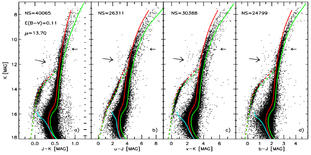
Figure 6.— From left to right NIR a) $K$, J–K, and Strömgren –NIR b) $K$, u–J; c) $K$, $v-K$; d) $K$, b–JCMDs of $\omega$ Cen. Stars are selected according to photometric accuracy $\sigma_{J,K,u,v,b}\leq 0.05$ mag and separation $sep_{K_{s}}$ > 5. Cluster isochrones, ZAHBs, true distance and reddening are the same as in Fig. 5. The error bars in the left panel show the mean intrinsic error in color at different $K$ magnitudes. The small horizontal arrows mark the location of the $\,\omega$ 3  metal-rich RGB, while the other arrows display the reddening vector.

5. Selection of RG stars

To study the $\omega$ Cen RG metallicity distribution, we selected only stars with magnitudes $y\lesssim$ 16.5 mag, ending up with a sample of $\approx$ 13,000 stars. However, in order to avoid subtle systematic uncertainties in the metallicity estimates, this sample needs to be purged of the contamination of field stars. To do this we used the optical-NIR color-color planes suggested by CAS07 and by CA07. The Strömgren photometry was cross-correlated with our NIR photometry in the central cluster regions (FOV $\approx 13\arcmin\times 13\arcmin$, see Fig. 2), while for the external regions we adopted the Two Micron All Sky Survey (2MASS) NIR catalog (see §2.2). The 2MASS catalog has an astrometric precision of $\sim$ 100 mas, and the magnitude limit ranges from $\sim 14.3$ for the $K$-band to $\sim 15.8$ for the $J$-band. In $\omega$ Cen these magnitude limits fall near the base of the RGB and the TO. The positional cross-correlation was performed with DAOMASTER, and we ended up with a sample of $\sim$ 64,000 stars having measurements in at least three of the four Strömgren bands and at least two of the three NIR bands.

Fig. 6 shows representative optical-NIR CMDs, namely $K$, u–J (panel b), $K$, v–K (panel c), and $K$, b–J (panel d). The temperature sensitivity of optical-NIR colors is quite large, and indeed the u–J  color increases by eight magnitudes when moving from hot HB stars (u–J$\sim 0$) to cool giant stars (u–J$\geq 8$) near the RGB tip. The same applies to the v–K  color, where the aforementioned star groups span a range of $\approx 7$ mag. In particular, the discrete nature of $\omega$ Cen RGBs (S05a) and the split between AGB and RGB stars can be easily identified in the three optical-NIR CMDs. The red and green lines display the same cluster isochrone as in Fig. 5, and they correspond to the same distance modulus and extinction coefficients. Data plotted in Fig. 6 show that, within the current uncertainties, theory and observations agree quite well. It is worth noting that BSs in the $K$, b–J CMD (panel d) form a spur of blue stars well separated from the bulk of the old population at $K\sim 16.5$, b–J$\sim$0.9. A more detailed comparison between theory and optical-NIR data will be discussed in a future paper.

In what follows, we have adopted the v–Kvs u–Jcolor-color plane to fully exploit the temperature sensitivity of optical-NIR colors in distinguishing cluster from field stars.

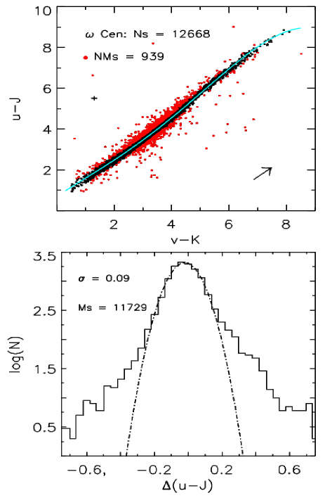
Figure 7.— Top: $\omega$ Cen RG stars plotted in the $(\hbox{\it u--J\/},\,\hbox{\it v--K\/})$ plane. The error bars display the mean photometric error in the adopted colors. Red dots are candidate field stars (Non-Member stars, NMs = 939). The solid turquoise line is the fitted cluster fiducial sequence. Bottom: logarithmic distribution of the difference between the u–J color of individual stars and the u–J color of the fiducial cluster sequence. The dashed-dotted line displays the Gaussian function that fits the color difference distribution. Objects with $\Delta(\hbox{\it u--J\/})\leq 2.5\times\sigma_{\hbox{\it u--J\/}}$ were considered candidate $\omega$ Cen RG stars (Member stars, Ms = 11,729).

We first selected RG stars with measurements in the four Strömgren bands ($u,v,b,y$) and two NIR bands ($J,K$), ending up with a sample of more than 12,000 stars (see top panel of Fig. 7). To define the fiducial cluster sequence in the $\hbox{\it u--J\/},\,\hbox{\it v--K\/}$ plane we selected the stars at distances from 0^′.5 to 1^′ from the cluster center (see black dots in the top panel of Fig. 7). In this plane the distribution of the cluster RG sequence is not linear, so we adopted a fourth-order polynomial to represent the RGB. Then, we estimated the difference in color between individual RG stars and the u–J color of the fiducial line at the same v–K color. The bottom panel of Fig. 7 shows the logarithmic distribution of the color excess $\Delta(\hbox{\it u--J\/})$ for the entire sample. We fitted the distribution with a Gaussian function and we considered only those stars with $\Delta(\hbox{\it u--J\/})\leq 2.5\times\sigma_{\hbox{\it u--J\/}}$ as bona fide $\omega$ Cen RG stars. The red dots in the top panel of Fig. 7 mark the candidate field stars after this selection.

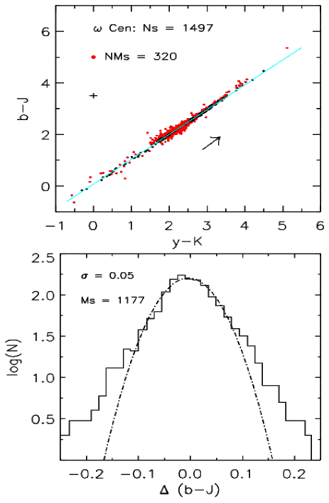
Figure 8.— Top: $\omega$ Cen RG stars plotted in the $(\hbox{\it b--J\/},\,\hbox{\it y--K\/})$ plane. The error bars show the mean photometric error in the adopted colors. Red dots are candidate field stars (NMs = 320). The solid turquoise line is the fitted cluster fiducial sequence. Bottom: logarithmic distribution of the difference between the b–J color of individual stars and the b–J color of the fiducial cluster sequence. The dashed–dotted line displays the Gaussian function that fits the distribution of the difference in color. Objects with $\Delta(\hbox{\it b--J\/})\leq 1.5\times\sigma_{\hbox{\it b--J\/}}$ were considered candidate $\omega$ Cen RG stars (Ms = 1,177).

Subsequently, we selected only stars from the MH data set with measurements in the Strömgren $v,b,y$ bands (1497 RGs) and in the $J,K$ NIR bands that were not included in the previous selection. In this case, we adopted the $\hbox{\it b--J\/},\,\hbox{\it y--K\/}$ plane to clean the RG sample of field star contamination. Fig. 8 shows the selected stars plotted in this plane, and the logarithmic distribution (bottom panel) of the color excess $\Delta(\hbox{\it b--J\/})$. In fitting the distribution with a Gaussian function, we considered only those stars having $\Delta({\hbox{\it b--J\/}})\leq 1.5\times\sigma_{\hbox{\it b--J\/}}$ as bona fide $\omega$ Cen RG stars. The red dots in the top panel of Fig. 8 mark the candidate field stars in this sample. Since we applied different selection criteria to the different samples, we ended up with a total of $\sim 12,900$ RGs with a measurement in at least three Strömgren bands and in two NIR bands. The original sample was thus reduced by roughly 10%.

Subsequently, in order to improve the selection of candidate field stars we also re-identified a subsample of our optical catalog in the proper motion catalog of van Leeuwen et al. (2000, hereinafter LE00). The average proper-motion precisions in this catalog range from 0.1 mas yr^-1 to 0.65 mas yr^-1 from the brightest to the faintest stars ($V\sim 20$ mag). The average positional errors are 14 mas. The cross identification was performed in several steps: (1) the IRAF/IMMATCH package was used to establish a preliminary spatial transformation from the Strömgren catalog CCD coordinates to the reference catalog equatorial (J2000.0) system for a subsample of matched stars; (2) the full Strömgren catalog was transformed onto and matched with the reference catalog on the basis of positional coincidence and initially also on apparent stellar brightness; (3) the previous steps were reiterated two or three times until the ultimate transformation permitted a near-complete matching, and then (4) the final, matched sample of common stars excluded entries separated by more than 0.56”. This provided us with reliable equatorial coordinates and proper motions for matching stars in the Strömgren data set.

Then, we performed a selection by proper motion. In particular, we considered as cluster members those stars with membership probabilities (see LE00) higher than 65%. This additional selection further decreased the sample of candidate RG members by $\approx$ 2%. The final catalog includes $12,700$ probable $\omega$ Cen RG stars.

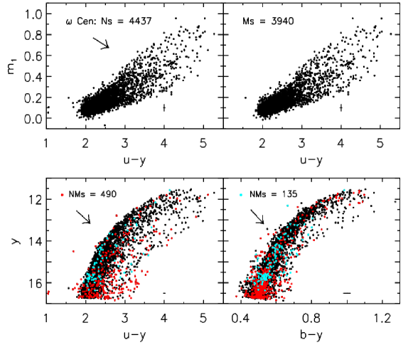
Figure 9.— Top: $\omega$ Cen RG stars selected in photometric error ($\sigma_{v,b,y}\leq$ 0.015 mag) and separation ($sep_{v,b,y}\geq$ 3) and plotted in the $m_{1},\,\hbox{\it u--y\/}$ plane (left). The right panel shows candidate $\omega$ Cen RG stars (Ms = 3,940) plotted in the same plane. Candidate cluster stars were selected according to optical–NIR colors ($\Delta(\hbox{\it u--J\/})\leq 2.5\times\sigma_{\hbox{\it u--J\/}}$ and $\Delta(\hbox{\it b--J\/})\leq 1.5\times\sigma_{\hbox{\it b--J\/}}$) and membership probability higher than 65%. Bottom: Strömgren CMDs $y$, u–y (left) and $y$, b–y (right) for cluster and field star candidates. The black dots mark candidate $\omega$ Cen RG stars, while red dots mark candidate field stars selected according to the optical–NIR color–color selection (NMs = 490). The turquoise dots mark probable field stars according to the proper motion selection (NMs = 135). The error bars account for uncertainties in intrinsic photometric errors. The arrows show the reddening vector.

Figure 10.— Radial distribution of candidate $\omega$ Cen RG stars (solid line) and of field stars (dashed line). The latter sample includes stars selected according to the optical–NIR color–color planes and to the proper motions.

To test the plausibility of the procedures adopted to disentangle $\omega$ Cen members from field stars, the top panels of Fig. 9 show from left to right the distribution in the $m_{1},\hbox{\it u--y\/}$ plane of the original RG sample selected by photometric precision ($\sigma_{v,b,y}\leq$ 0.015 mag and $sep_{v,b,y}\geq$ 3) and of the sample after the selection in the optical-NIR color-color plane. Fig. 9 shows that $\omega$ Cen RGs do not follow a well-defined sequence on the $m_{1},\hbox{\it u--y\/}$ plane, as the other GCs do (see CA07). The RG stars in $\omega$ Cen show a wide spread in color that cannot be explained as photometric errors or differential reddening (see the error bars and the reddening vector plotted in Fig. 9). The bottom panels of Fig. 9 show the same RG sample (black dots) plotted in the $y$, u–y (left) and in the $y$, b–y (right) CMDs; overplotted are the candidate field stars after the selection in the optical-NIR color-color plane (red dots), and after the selection by proper motion (turquoise dots). It is noteworthy that most of the field stars have magnitudes and colors that are very similar to the probable cluster RG stars.

As a final validation of the two selection procedures, we compared the radial distribution of candidate $\omega$ Cen RGs and field stars. Fig. 10 shows the two logarithmic distributions and the flat trend of field stars (dashed line) is quite evident when compared with the steeper and more centrally concentrated distribution of likely $\omega$ Cen stars (solid line). It was already noted by CA07 that the mild decrease in the number of apparent field stars in the outskirt of the cluster suggests that our color-color selection is very conservative, and some real cluster members have probably been erroneously rejected. However, in these photometric selections it is more important to keep the probable nonmembers out than to keep probable members in (ATT00).

6. A new calibration of the $m_{1}$, b–y metallicity relation

In CA07 we provided new empirical and semi-empirical calibrations of the $m_{1}$ metallicity index based only on cluster RG stars. These new MIC relations were then validated on the basis of GC and field RGs with known spectroscopic iron abundances in the Zinn & West (1984) metallicity scale, and were found to provide metallicity estimates with an accuracy of the order of 0.2 dex. The main difference between the CA07 MIC relations and similar relations available in the literature is that the former adopt the u–y and v–y colors instead of b–y. The main advantage of the u–y and v–y colors is the stronger temperature sensitivity, and the MIC relations show a linear and well-defined slope in the $m_{1},\hbox{\it u--y\/}/\hbox{\it v--y\/}$ planes. However, the u–y and the v–y colors also have a drawback: they are affected by carbon (C) and/or nitrogen (N) enhancements (CA07). To investigate the different behavior of the u–y, v–y, and b–y colors as a function of the CH and the CN abundances, we also performed a metallicity calibration based on the b–y color. We found that this MIC relation shows a nonlinear trend over the typical color range of RG stars, namely $0.42<(\hbox{\it b--y\/})_{0}<1.05$ (see Fig. 2 of Calamida et al. 2007b, hereinafter CA07b). Therefore, we included a quadratic color term to characterize the calibration (see also HR00 and CA07b). Specifically, we estimated a semi-empirical calibration based on the b–y color of the theoretical evolutionary models by Pietrinferni et al. (2006) for an $\alpha$-enhanced ($\hbox{\rm[$\alpha$/Fe]}=0.4$) mixture. Theoretical predictions were transformed to the observational plane with the semi-empirical Color-Temperature Relations (CTRs) provided by Clem et al. (2004). We adopted the procedure described in CA07 and applied a multilinear regression fit to estimate the coefficients of the MIC relation:

$$m_{0}=\alpha+\beta\,\hbox{\rm[Fe/H]}+\gamma\,CI_{0}+\delta\,\hbox{\rm[Fe/H]}\,CI_{0}+\epsilon\,CI_{0}^{2}+\zeta\,\hbox{\rm[Fe/H]}\,CI_{0}^{2}$$ (1)

where $m_{0}$ = $m_{10}$ and $CI_{0}$ are the unreddened color indices. Similar relations were also derived for the reddening-free $[m]=m_{1}+0.3\times(b-y)$ index. Together with the calibration of semi-empirical MIC relations we performed an independent empirical calibration using the observed colors of RG stars in selected GCs, M92, M13, NGC 1851, NGC 104, for which accurate Strömgren photometry is available (Grundahl et al. 1998; CA07). These GCs cover a broad range in metal abundances ($-2.2<\hbox{\rm[Fe/H]}<-0.7$) and are minimally affected by reddening ($E(\hbox{\it B--V\/})\leq 0.04$). The coefficients of the fit of both semi-empirical and empirical MIC relations are listed in Table 11. In order to validate the new MIC relations we decided to apply them to nine GCs for which accurate Strömgren photometry, absolute calibration, and sizable samples of RG stars are available. They are M92, NGC 6397, M13, NGC 6752, NGC 1851, NGC 288, NGC 362, M71 and NGC 104. Table 12 lists spectroscopic and photometric metallicities for these clusters. Note that five out of the nine GCs had been adopted to calibrate the empirical MIC relations. We find a good agreement for both the empirical and the semi-empirical MIC relations. The comparison between the mean photometric metallicity estimates and the spectroscopic measurements indicates that they agree with each other within $1\sigma$ uncertainties. It is noteworthy that the accuracy of photometric metallicity estimates applies not only to metal-intermediate clusters with low reddening corrections (NGC 288, $E(B-V)\sim 0.02$), but also to more metal-rich clusters with high reddening (M71, $E(B-V)\sim 0.30$, Harris 1996).

To further constrain the calibration of the new MIC relations we decided to compare them with $m_{0},(\hbox{\it b--y\/})_{0}$ metallicity calibrations available in the literature. We adopted the field RG sample by Anthony-Twarog & Twarog (1994, hereinafter ATT94) and Anthony-Twarog & Twarog (1998, hereinafter ATT98), already used by CA07. The interested reader is referred to this paper for more details concerning the selection of the RG sample.

We compared the photometric metallicities of 59 out of the 79 stars for which ATT94 provided an estimate. The spectroscopic and the photometric metallicity distributions are in fair agreement. The mean differences are $0.02\pm 0.03$, with a dispersion of $\sigma$ = 0.22 dex (ATT94) and $0.13\pm 0.03$, with a dispersion of $\sigma$ = 0.20 dex (H00). The small difference between the current errors and the original ones derived by ATT94 and H00 is only due to the different selection criteria. The mean differences using the same 59 stars and current empirical and semi-empirical MIC relations are $-0.12\pm 0.02$ and $-0.15\pm 0.02$ dex, with a dispersion of $\sigma$ = 0.15 and of $\sigma$=0.18 dex, respectively. Fig. 11 shows the comparison between the spectroscopic metallicity distribution (dashed line) and the metallicity distribution obtained with the empirical MIC relation based on the ($m_{0},(\hbox{\it b--y\/})_{0}$) calibration by ATT94. The middle panel shows the comparison with the metallicity distribution based on our empirical and semi-empirical ($m_{0},(\hbox{\it b--y\/})_{0}$) MIC relations for the complete sample of 79 RG stars. The bottom panel shows the comparison with the metallicity distribution based on the empirical MIC relation ($m_{0},(\hbox{\it b--y\/})_{0}$) provided by H00 for 73 out of the 79 RG stars with $-2.3<\hbox{\rm[Fe/H]}<-0.4$. Data plotted in the top and in the middle panel of Fig. 11 indicate that spectroscopic and photometric metallicity distributions agree quite well. The metallicity distribution based on the H00 calibration appears slightly more metal-rich ($\sim$ 0.13 dex). These data show that metal-abundance estimates for the ATT98 sample based on the ($m_{0},(\hbox{\it b--y\/})_{0}$) MIC relations are shifted by $\sim$ -0.14 dex, as already found by CA07 for empirical and semi-empirical ($m_{0},(\hbox{\it v--y\/})_{0}$; $m_{0},(\hbox{\it u--y\/})_{0}$) relations. They suggested that this difference might be due the different approach (cluster vs field RGs) in the calibration of the $m_{1}$ index. In spite of this systematic difference, the intrinsic dispersion of the difference between photometric and spectroscopic metallicities is smaller than 0.2 dex, and it is mainly due to photometric, reddening, and spectroscopic errors (see Fig. 2 of CA07b).

Figure 11.— Comparison between spectroscopic and photometric metallicity distributions based on the 79 field RG stars from the ATT94 and ATT98 sample (dashed line) versus the spectroscopic iron abundance. Top: the solid line shows the metallicity distribution based on the ATT94 empirical –$m_{0},(\hbox{\it b--y\/})_{0}$– MIC relation. Middle: the solid and the dashed-dotted lines display the metallicity distributions based on our empirical and semi-empirical –$m_{0},(\hbox{\it b--y\/})_{0}$– MIC relations. Bottom: the solid line shows the metallicity distribution based on the H00 empirical –$m_{0},(\hbox{\it b--y\/})_{0}$– MIC relation.

7. Comparison between photometric and spectroscopic iron abundances

To estimate the metal content of the selected $\omega$ Cen RG stars we adopted the MIC relations provided by CA07 (see their Table 3) and based on the u–y and on the v–y color, together with the new MIC relation derived in §6. The photometric metallicities were estimated using both the empirical and the semi-empirical calibrations.

Figure 12.— Difference between photometric and spectroscopic metallicities, $\Delta\hbox{\rm[Fe/H]}\equiv\hbox{\rm[Fe/H]}_{phot}-\hbox{\rm[Fe/H]}_{spec}$, plotted versus $\hbox{\rm[Fe/H]}_{spec}$. Spectroscopic iron abundances for 39 ROA stars come from the list of ND95 (filled circles), eight from the list of PA02 (open circles), and four from the list of SM00 (open triangles). Solid lines connect RGs with spectroscopic measurements from different authors. Panels a) and b) display the differences for two empirical calibrations ($m_{0},(\hbox{\it v--y\/})_{0}$; $[m],(\hbox{\it v--y\/})_{0}$), while the panels c) and d) show the differences for the same MIC relations, but based on the semi-empirical calibrations. Crosses mark CN-strong stars according to ND95. The error bars in the top panel represent photometric and spectroscopic errors.

The individual metallicities were estimated by assuming for $\omega$ Cen a mean reddening value of $E(B-V)$ = 0.11 (CA05) and the extinction coefficients for the Strömgren colors discussed in §4.

To verify the accuracy of the metallicity estimates, we cross-correlated our RG sample with the iron abundances—based on high-resolution spectra—of 40 ROA stars provided by ND95. We found 39 RG stars in common. Moreover, we matched our photometric catalog with the iron abundances—again based on high-resolution spectra—of ten metal-rich RGs provided by PA02. Two of these stars (ROA 179, 371), are also in the ND95 sample. We also adopted the iron abundances provided by SM00 for four RGs in common with the ND95 sample (ROA 102, 213, 219, 253) based on similar high-resolution spectra. We ended up with a sample of 47 RGs with accurate iron measurements for which we have either three (47, $vby$) or four (28, $uvby$) independent Strömgren magnitudes. The difference between the inferred photometric metallicities and the spectroscopic measurements are plotted versus spectroscopic abundances in Fig. 12. The four different panels display metallicity estimates based on different empirical MIC relations. Data plotted in this figure indicate that photometric and spectroscopic abundances are in reasonable agreement. The mean difference for the four MIC relations is $<\Delta\hbox{\rm[Fe/H]}>=<\hbox{\rm[Fe/H]}_{phot}-\hbox{\rm[Fe/H]}_{spec}>$= 0.17$\pm$0.01 dex, with a dispersion of the residuals of $\sigma$ = 0.31 dex. Once we remove CN-strong and chemically peculiar stars (vide infra), the scatter around the mean is mainly due to photometric and spectroscopic measuring errors. The error bars on the top panel of Fig. 12 display the entire error budget. Note that throughout the paper with the symbol $\hbox{\rm[Fe/H]}_{phot}$ we mean the overall stellar metallicity, i.e., the sum of all elements beyond helium (VandenBerg et al. 2000).

Uncertainties in reddening corrections minimally affect the current metallicity estimates, and indeed the photometric metallicities based on the reddening-free metallicity index, $[m]$, have similar differences and dispersions (panels b, d). The same outcome applies to photometric metallicities based on empirical and on semi-empirical MIC calibrations. However, eight RG stars with iron abundance ranging from $\hbox{\rm[Fe/H]}_{spec}=-1.7$ to –0.9 (ROA 53, 100, 139, 144, 162, 253, 279, 480) present larger ($\Delta\hbox{\rm[Fe/H]}>$ 0.3 dex) differences. Interestingly, six of them (marked with crosses in Fig. 12) are CN-strong stars, while ROA 279 (marked with an asterisk) is a CH-star (see, e.g. ND95). The CN-weak star ROA 53 has $\Delta\hbox{\rm[Fe/H]}\approx$ 0.8 dex, but the photometric metallicity is probably affected by poor photometric precision ($\sigma_{v,b,y}\sim$ 0.05). The other three discrepant stars, with $\hbox{\rm[Fe/H]}_{spec}\geq-1.0$ belong to the PA02 sample. However, the PA02 spectroscopic measurements for the two ROA stars in common with ND95 are more metal-rich by $\approx$ 0.2 dex. This systematic difference has already been discussed by PA02. On the other hand, the iron abundances provided by ND95 and SM00 for the same RGs agree within the uncertainties. This suggests that these more metal-rich discrepant objects deserve further investigation.

If we neglect the CN-strong stars, the CH-star, the ROA53, and the three stars from the PA02 sample, the mean difference for the four MIC relations is $0.02\pm 0.02$ dex, with a dispersion of the residuals of $\sigma$ = 0.16 dex.

Figure 13.— Same as Fig. 12, but for the 28 stars for which the $u$-band photometry is available. Photometric metallicities are based on four different MIC relations ($m_{0},(\hbox{\it u--y\/})_{0}$; $[m],(\hbox{\it u--y\/})_{0}$). Crosses mark CN-strong stars according to ND95, while the plus marks the candidate CN-strong star ROA 248.

To further constrain the plausibility of our findings, we performed the same comparison using 28 stars for which $u$-band photometry is available. Fig. 13 shows the difference between photometric and spectroscopic abundances using both empirical (panels a,b) and semi-empirical (panels c,d) calibrations ($m_{0},(\hbox{\it u--y\/})_{0}$; $[m],(\hbox{\it u--y\/})_{0}$). The result is quite similar to the MIC relation based on the v–y color, and indeed the mean difference is $<\Delta\hbox{\rm[Fe/H]}>$ = 0.26$\pm$0.02 dex, and the dispersion of the residuals is $\sigma\sim$ 0.36 dex. The star ROA 248 ($\hbox{\rm[Fe/H]}=-0.78$ dex) shows a large discrepancy ($\Delta\hbox{\rm[Fe/H]}\approx 0.6$). However, ROA 248 could be a candidate CN-strong star, as suggested by the large value of the cyanogen index, S3839 = 0.51 (ND95), and by its peculiar position in the $m_{0},(\hbox{\it v--y\/})_{0}$ plane and in the $y_{0},(\hbox{\it v--y\/})_{0}$ CMD (see Fig. 14). If we neglect the five CN-strong stars, the stars ROA 248, ROA 53, and the three stars from PA02, for which the discrepancy in this plane is even larger, the mean difference for the four MIC relations is $0.07\pm 0.03$ dex, with a dispersion of $\sigma$ = 0.16 dex.

We performed the same test using the empirical and the semi-empirical $m_{0},(\hbox{\it b--y\/})_{0}$ MIC relations and we found that the mean difference over a sample of 47 objects is $<\Delta\hbox{\rm[Fe/H]}>$ = 0.22$\pm$0.05 dex, and the dispersion of the residuals is $\sigma\sim$ 0.43 dex. Once we remove the objects with peculiar abundances we find $<\Delta\hbox{\rm[Fe/H]}>$ = 0.01$\pm$0.03 dex, and the dispersion of the residuals is $\sigma\sim$ 0.24 dex.

To avoid subtle uncertainties caused by the limited sample of RG stars with accurate spectroscopic measurements, we took advantage of the recent large sample of iron abundances, based on high-resolution spectra for 180 RG stars in $\omega$ Cen, collected by Johnson et al. (2008, hereinafter J08). This catalog was cross-correlated with the proper motion measurements by LE00 and we considered as candidate cluster stars those with a proper motion probability of 80%. We cross-correlated this spectroscopic sample with our photometric catalog and we found 118 RGs in common. We estimated the difference between photometric ($m_{0},\hbox{\it v--y\/}_{emp}$) and spectroscopic metallicities and found a mean difference of $0.05\pm 0.02$ dex, with a dispersion of the residuals of $\sigma$ = 0.36 dex.

To constrain on a quantitative basis the impact of possible CN enhancements we supplemented previous spectroscopic catalogs with the large set of medium-resolution spectra collected by VL07 (for more details see §9). We found 373 RGs in common with our photometric catalog.

Figure 14.— Difference between photometric and spectroscopic metallicities, $\Delta\hbox{\rm[Fe/H]}=\hbox{\rm[Fe/H]}_{phot}(m_{0},\hbox{\it v--y\/}_{0})_{emp}-\hbox{\rm[Fe/H]}_{spec}$, plotted versus $\hbox{\rm[Fe/H]}_{spec}$ for the 118 RG stars with accurate iron abundances by J08. Filled circles mark stars with the measurement of the spectroscopic $S3839$ index (VL07), while those for which this measurement is not available are marked with open circles. Crosses mark CN-strong stars according to both our selection (see §9) and to ND95. The error bars account for both photometric and spectroscopic errors. The mean difference is $\sim 0.05\pm 0.03$ dex, with a dispersion in the residuals of $\sigma=0.37$ dex. The stars with $\Delta\hbox{\rm[Fe/H]}\geq 0.3$ dex are either CN-strong or do not have a spectroscopic CN-band measurement.

Fig. 14 shows the difference between photometric and spectroscopic iron abundances for the 118 RGs in common with J08. Filled circles mark the stars for which the measurement of the $S3839$ index (cyanogen band) is available (VL07), while the open circles represent stars which lack of this measurement. The crosses mark the CN-strong stars according to either our selection ($\delta CN>0.2$, see §9) or to that of ND95. Data plotted in this figure show that CN-strong stars are, as expected, concentrated among the more metal-rich stars ($\hbox{\rm[Fe/H]}\gtrsim-1.5$, Gratton, Sneden & Carretta 2004). The mean difference between photometric and spectroscopic abundances, using the six different MIC relations, is $\Delta\hbox{\rm[Fe/H]}=0.05\pm 0.03$ and $\sigma=0.37$ dex. Once again we found that the dispersion of the residuals is larger in the $m_{0},(\hbox{\it b--y\/})_{0}$ than in the $m_{0},(\hbox{\it v--y\/})_{0}$ relation ( 0.36 vs 0.42, empirical; 0.33 vs 0.40, semi-empirical).

It is worth mentioning that 25 out of the 118 stars show discrepancies in iron abundance larger than 0.3 dex. The measurement of the CN index is available for thirteen of these stars and among them ten are CN-strong. If we move the limit down to 0.2 dex, the number of discrepant stars is 46, and the CN index is available for 20 of them. The fraction of CN-strong stars becomes of the order of 75%. On the other hand, 17 stars appear to be under-abundant in iron by more than 0.3 dex; among them ten have measurements of the CN index and only one is a CN-strong star. The current findings thus indicate that stars with large positive discrepancies in the photometric metallicity are highly correlated with the occurrence of strong CN bands. The stars with large negative discrepancies require a more detailed spectroscopic investigation to constrain their abundance pattern. If we neglect the CN-strong stars we find a mean difference of $\Delta\hbox{\rm[Fe/H]}=0.02\pm 0.04$ and $\sigma=0.37$ dex (93 stars).

As a final test of the intrinsic accuracy of the photometric abundances, we plotted the 118 RGs by J08 (open circles), the 39 ROA stars (open triangles) and the 8 RGs by PA02 (open diamonds) onto the $m_{0},(\hbox{\it v--y\/})_{0}$ plane (Fig. 15, top panel). The spectroscopic stars have the expected $m_{0}$/color distribution with the eight metal-rich RGs by PA02 attaining the largest $m_{0}$ values and color the faintest apparent $y_{0}$ magnitudes at fixed color (bottom panel). The plausibility of their metal-rich nature is also supported by the fact that six of them are located along the anomalous RGB ($\,\omega$ 3). It is noteworthy that CN-strong stars (crosses) possess intermediate $m_{0}$ values and apparent $y_{0}$ magnitudes. This finding should not be affected by selection effects, since the low-resolution spectra collected by V07 cover a significant fraction of the RG branch in $\omega$ Cen (down to V$\sim$16). The same outcome applies for the CH-star (asterisk), while the candidate CN-strong star ROA 248 (plus) shows the largest $m_{0}$ value and the reddest v–y color in the sample, thus supporting its peculiar nature.

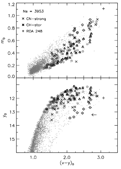
Figure 15.— Top: RG stars of $\omega$ Cen in the $m_{0},(\hbox{\it v--y\/})_{0}$ plane. The open circles mark the 108 RGs from J08, the open triangles mark the 39 ROA stars from ND95 and the diamonds the eight RGs from PA02. The CN-strong stars are marked with crosses, the CH-star (ROA 279) with an asterisk and the candidate CN-strong star (ROA 248) with a plus. Bottom: Same as the top, but in the $y_{0},(\hbox{\it v--y\/})_{0}$ CMD. The arrow indicates the metal-rich RGs located along the $\,\omega$ 3  branch.

The above results highlight three relevant findings: i)– Photometric iron abundances agree quite well with spectroscopic measurements, and indeed the mean difference is, within the errors, negligible. This supports the hypothesis suggested by CA07 (see also §6) that the discrepancy between photometric and spectroscopic abundances found for field RG stars is caused by an intrinsic difference in their abundance patterns. ii)– The MIC relations based on the $(\hbox{\it u--y\/})$ and the $(\hbox{\it v--y\/})$ color are more affected by C and N enhancements. Two strong CN absorption bands at $\lambda=4142$ and $\lambda=4215$ Å, are close to the effective wavelength of the $v$ ($\lambda_{eff}=4110$ Å) filter, while the two CN bands at $\lambda=3590$ and $\lambda=3883$ Å  affect the $u$ ($\lambda_{eff}=3450$ Å) filter (see e. g. Smith 1987; Bell & Gustafsson 1978; ATT94; H00; Grundahl et al. 2002; CA07). Although these MIC relations depend on CN both in the $m_{1}$ index and in the color, they provide more robust photometric abundances when compared with the $m_{0},(\hbox{\it b--y\/})_{0}$ relation, due to their stronger temperature sensitivity. iii)– The dispersion of the residuals between photometric and spectroscopic abundances is of the order of 0.3–0.4 dex. However, the dispersion decreases by at least a factor of two if all the stars appearing to have abundance anomalies (ND95 data) are removed from the sample.

8. Photometric metal abundance distributions

In the previous section we have investigated pros and cons of the different MIC relations to estimate the metal content of RG stars. To constrain the metallicity distribution of $\omega$ Cen RGs we selected the stars with photometric precision $\sigma_{v,b,y}\leq$ 0.015 and, $\sigma_{u}\leq$ 0.02 mag, and $sep>$ 3. Moreover, we excluded all the stars with colors redder/bluer than the color range covered by empirical and semi-empirical calibrations (CA07). We ended up with a sample of 3,953 RGs; among them 2,846 stars also have the $u$-band measurement. Independent estimates of the photometric metallicity were obtained from the three different MIC relations and the two calibrations. Fig. 16 shows the six different metallicity distributions for the selected RGs. The individual distributions were smoothed with a Gaussian kernel having a standard deviation equal to the photometric error in the $m_{1}$ index. To provide a robust fit of the metallicity distributions we developed an interactive program that performs a preliminary Gaussian fit of the main peaks. On the basis of the residuals between the metallicity distributions and the analytical fit, the software allow us to insert manually new Gaussian components. At each step, the code compute a new global solution and the procedure is iterated until the residuals are vanishing. We fit the distributions with a sum of seven Gaussians and the dashed lines plotted in Fig. 16 display the cumulative fits, while the asterisks mark the position of the different Gaussian peaks. The peaks and the sigma of the different Gaussian fits are listed in Table 13.

Figure 16.— Distribution of photometric iron abundances based on empirical (top) and semi-empirical (bottom) calibrations of different MIC relations. The sample size of the $m_{0},(\hbox{\it u--y\/})_{0}$ (left), of the $m_{0},(\hbox{\it v--y\/})_{0}$ (middle) and of the $m_{0},(\hbox{\it b--y\/})_{0}$ (right) relations are also labeled. The metallicity distributions were smoothed with a Gaussian kernel with a $\sigma$ equal to the individual intrinsic error on the $m_{1}$ index. The dashed line shows the fit of the metallicity distribution computed as the sum of seven Gaussians. The asterisks mark the peaks of the seven Gaussians. The vertical dotted lines display the different metallicity regimes: metal-poor (MP), metal-intermediate (MI), metal-rich (MR) and solar-metallicity (SM).

The shape of the metallicity distributions is, as expected, asymmetric with a sharp cut-off in the metal-poor tail ($\hbox{\rm[Fe/H]}_{phot}<$ –2) and a metal-rich tail approaching Solar iron abundances. The different MIC relations and the different calibrations show, within the errors, very similar metallicity distributions. The same conclusion applies to the peaks in the metallicity distribution (see Table 13). The peaks according to the six calibrations are located at $\hbox{\rm[Fe/H]}_{phot}=$ $-1.73\pm 0.08$, $-1.29\pm 0.03$, $-1.05\pm 0.02$, $-0.80\pm 0.04$, $-0.42\pm 0.12$ and $-0.07\pm 0.08$ dex, where the uncertainties are the standard errors of the mean. A handful of objects seems to show super-Solar iron abundance – $\hbox{\rm[Fe/H]}_{phot}\approx$ $0.24\pm 0.13$ –, but this sample vanishes in the $m_{0},\ (\hbox{\it u--y\/})_{0}$ distribution and might be caused by CN-strong stars of the metal-rich peak at $\hbox{\rm[Fe/H]}_{phot}\approx$ -0.07 dex. These findings are minimally affected by uncertainties in reddening corrections, since the metallicity distributions based on the reddening-free $[m]$ index are very similar (Calamida 2007).

The four most significant peaks ($-1.73\leq\hbox{\rm[Fe/H]}\leq-0.80$) in the photometric iron distributions agree quite well with the spectroscopic peaks measured by J08 (see their Fig. 10). Iron abundances based on high-resolution spectra also suggest the presence in $\omega$ Cen of more metal-rich stars ($\hbox{\rm[Fe/H]}=-0.60\pm 0.15$) stars (ND95; PA02; Pancino 2004). The outcome is the same if we compare photometric abundances with metallicity distributions based on low and medium resolution spectra. These investigations are typically based on measurements of the calcium triplet (N96, 517 RGBs; SK96, 343 RGBs; S05b, 152 SGBs; Stanford et al. 2006a, 442 MSs) that are transformed into iron abundances via empirical relations, or on direct iron line measurements (H04, $\sim$ 400 MSs and SGBs; van Loon et al. 2007, hereinafter VL07, $\sim$ 1500 HBs and RGBs; Villanova et al. 2007, 80 SGBs). In particular, the metal-rich tail in the metallicity distributions based on larger cluster samples approaches $\hbox{\rm[Fe/H]}\approx-0.5\pm 0.2$ dex. The metallicity distributions based on photometric indices (HR00, $m_{1}$-index, $\sim 1500$ RGs; Rey et al. 2000, $hk$-index 131 RR Lyrae; Hughes et al. 2004, $m_{1}$-index, $\sim 2500$ MSs, SGBs, RGBs) also provide similar results.

Figure 17.— Average distribution of photometric iron abundances based on the three empirical (top) and on the three semi-empirical (bottom) calibrations of the adopted MIC relations. The asterisks mark the peaks of the seven Gaussian adopted in the cumulative fit (dashed line). The vertical dotted lines display the mean of the different metallicity regimes identified in Fig. 16.

The large number of RGs allows us to identify four different metallicity regimes: metal-poor (MP) with $\hbox{\rm[Fe/H]}\lesssim-1.5$, metal-intermediate (MI) with $-1.5\lesssim\hbox{\rm[Fe/H]}\lesssim-1.0$, metal-rich (MR) with $-1.0\lesssim\hbox{\rm[Fe/H]}\lesssim-0.1$ and Solar metallicity with $\hbox{\rm[Fe/H]}\approx 0$ dex (see vertical dotted lines in Fig. 16). The limits of these metallicity regimes are arbitrary, though identified with the occurrence of either a local minimum or a shoulder in the metallicity distribution.

Following the anonymous referee suggestion we estimated the average metallicity distributions of both empirical and semi-empirical MIC relations (see Fig. 17). We performed on the average distributions the same Gaussian fits adopted for the individual distributions. Data plotted in Fig. 17 (see also Table 13) show that both the peaks and the metallicity regimes are, within the errors, quite similar. The difference between the cumulative fits and the metallicity distributions suggests the possible occurrence of a secondary peak located at the edge between the MR and SM regime ($[Fe/H]\sim-0.25$).

The main findings concerning the metallicity distributions in $\omega$ Cen according to the photometric abundance estimates are the following:

i) The metallicity distribution shows a very sharp cutoff in the metal-poor regime, and the fraction of stars more metal-poor than $\hbox{\rm[Fe/H]}\approx-2.0$ dex is vanishing.

ii) The main iron peak is located at $\hbox{\rm[Fe/H]}\approx-1.73\pm 0.08$ dex, and the weighted mean fraction of stars in this metal-poor regime ($\hbox{\rm[Fe/H]}\leq-1.49$) is $\sim 39\pm 1$%. However, four out of the six metallicity distributions show either a double peak or a shoulder ($m_{0},(\hbox{\it u--y\/})_{0}$; $m_{0},(\hbox{\it v--y\/})_{0}$, see Fig. 16). The distance between the two peaks is on average of the order 0.2 dex. The large number of stars per bin and the minimal impact of CN-strong stars in this metallicity range suggest that the split is real.

iii) The metal-intermediate regime ($-1.49<\hbox{\rm[Fe/H]}\leq-0.93$) includes two secondary peaks ($\hbox{\rm[Fe/H]}\approx-1.29\pm 0.03$ [MI1], $-1.05\pm 0.03$ [MI2] dex) and a weighted mean fraction of stars of $\sim 32\pm 1$%.

iv) The metal-rich regime ($-0.93<\hbox{\rm[Fe/H]}\leq-0.19$) also includes two secondary peaks ($\hbox{\rm[Fe/H]}\approx-0.80\pm 0.04$ [MR1] $-0.42\pm 0.13$ [MR2] dex) and has a weighted mean fraction of stars of $\sim\;19\pm 4$%. In the spectroscopic metallicity distributions available in the literature, the last two peaks become more evident as soon as the sample size becomes of the order of several hundred stars.

v) In the solar metallicity regime ($\hbox{\rm[Fe/H]}\approx 0$) two secondary peaks are also present ($\hbox{\rm[Fe/H]}\approx-0.07\pm 0.08$ [SM1], $0.24\pm 0.13$ [SM2] dex), but only with a small fraction of stars ($\sim\;8\pm 5$%). This tail should be treated with caution, since we still lack firm spectroscopic evidence for the presence of RGs with solar iron abundances in $\omega$ Cen . Moreover, we cannot exclude the possibility that these objects either are affected by strong C and/or N enhancements, or belong to the Galactic field population.

vi) The difference in iron content among the individual peaks is roughly constant and equal to a factor of 3–4 (–1.7, –1.2, –0.6, and 0 on the logarithmic abundance scale).

vii) The fraction of stars belonging to the different metallicity regimes steadily decreases when moving from the metal-poor to the metal-rich domain. The relative fractions based on the different photometric diagnostics are in fair agreement (see Table 14). There are three exceptions. a) The $m_{0},(\hbox{\it u--y\/})_{0}$ indicates a larger fraction of MP stars when compared with the other MIC relations ($48\pm 2$% vs $38\pm 1$%). The difference might be due to the stronger sensitivity of this color in the faint RG limit (see left panel of Fig. 18 and Fig. 11 in CA07). To validate this working hypothesis we estimated the same fractions using only bright RGs ($y_{0}\leq 15$) and we found that the new values, within the uncertainties, agree quite well ($52\pm 2$% vs $49\pm 2$%). This evidence suggests that the current fraction of MP stars should be considered as a lower limit. b) The $m_{0},(\hbox{\it v--y\/})_{0}$ indicates a larger fraction of MR stars when compared with the other MIC relations ($24\pm 1$% vs $17\pm 1$%). The difference is almost certainly due to the stronger sensitivity of this color to CN-strong stars. This hypothesis is also supported by the slow decrease that the metallicity distribution shows in this abundance interval (see the middle panels in Fig. 16). c) The $m_{0},(\hbox{\it b--y\/})_{0}$ diagram indicates a significantly larger fraction of SM stars when compared with the other MIC relations ($14\pm 1$ vs $6\pm 1$%). The difference is due to the lesser sensitivity of this color in the metal-rich regime (see right panel in Fig. 18).

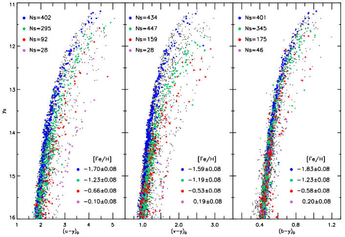
Figure 18.— Unreddened Strömgren CMDs for RGs characterized by different mean iron abundances. The blue dots mark metal-poor (MP) RGs, the green dots metal-intermediate (MI) RGs, the red dots metal-rich (MR) RGs and the purple dots the solar metallicity (SM) RGs. The individual sample sizes and the metallicity intervals are labeled.

Current findings agree well with the metallicity distribution function obtained by S05a using broad band photometry of RG stars (1364). In particular, they found a well defined MP peak ($Fe/H]\approx$-1.6 dex), three MI peaks ($Fe/H]\approx$-1.4,-1.1,-0.9 dex) and a sharp peak in the MR tail ($Fe/H]\approx$-0.6 dex, see their Fig. 8). The same outcome applies to the relative fraction of RG stars in the quoted metallicity regimes (see their Table 2).

To test the plausibility of the selected metallicity regimes, Fig. 18 shows the distribution of four different stellar groups with different mean metal abundances in three different CMDs. The MP sample are RGs located around the main peak, i.e., $\hbox{\rm[Fe/H]}\approx-1.70\pm 0.08$, while the other samples are located near other three main peaks: MI for $\hbox{\rm[Fe/H]}\approx-1.23\pm 0.08$, MR for $\hbox{\rm[Fe/H]}\approx-0.66\pm 0.08$ and SM for $\hbox{\rm[Fe/H]}\approx-0.1\pm 0.08$ dex. Data plotted in the left panel show a well defined u–y-color ranking over the entire magnitude range when moving from the metal-poor (blue dots) to the metal-intermediate (green dots), metal-rich (red dots) and solar metallicity (purple dots) RGs. The result is the same for the v–y–color (middle panel), but the solar metallicity stars located along the $\,\omega$ 3  branch show a larger color scatter and the four different groups merge in the faint magnitude range ($y_{0}<15$). The degeneracy becomes more evident when moving to the b–y–color (right panel).

The anonymous referee raised the problem that the CN molecular bands affect the Stroemgren u and v bands. Therefore, the Stroemegren MIC relations cannot be adopted to estimate [Fe/H] values in complex systems unless one has a knowledge of the strength of those CN bands. However, some circumstantial evidence move against this working hypothesis.
i)– In this investigation we are not attempting to estimate an iron content that is identical to the iron abundance measured by spectroscopist using high-resolution spectra. We have clearly stated that with [Fe/H], we mean a global metallicity, i.e., the sum of all elements beyond helium without explicit assumptions concerning the relative distribution among those elements. Plain physical arguments indicate that the sensitivity of the Stroemgren indices to metallicity comes from changes to the stellar structure —such as envelope opacity, and consequently stellar radius as a function of luminosity—and not merely from atmospheric spectral features. For this reason, a photometric index representing ”all metals” is a crude zero-th order estimate of the chemical content of a star. These metallicity estimates are adopted to rank RG stars according to their heavy element content and to detect sample of stars characterized by different relative ”metal” abundances.
ii)–The occurrence of strong molecular bands increases the dispersion in the mapping of heavy element abundances. However, even though the Stroemgren indices do not provide an exact equivalence with the iron abundance they still give a meaningful correlation with the star global metallicity. The precence of this correlation is supported by these evidence: a)– metallicity distributions based on MIC relations, with different sensitivities to the CN molecular bands, show similar peaks and valleys (see Fig. 16); b)– the position of peaks and valleys in the mean metallicity distributions (see Fig. 17) are, within the errors, very similar to the individual ones; c)– the RG stars show a well defined drift in color in the CMD, when moving from metal-poor to metal-rich stars (sse Fig. 18); d)– the main peaks of current metallicity distributions agree quite well with spectroscopic measurements. These findings indicate that metallicity estimates based on Stroemgren MIC relations are a robust diagnostic to identify stellar populations characterized by different global metallicities.
iii)– Accurate spectroscopic measurements indicate variations in the heavy element abundance on a star-by-star basis in all GCs. Together with changes in the relative abundances of CNO elements, well defined anticorrelations have been found between O and Na and between Mg and Al. Field RG stars do not show the above chemical anomalies (Gratton, Sneden, & Carretta 2004). To provide homogeneous metallicity estimates of cluster RGs we provided new calibrations of the Stroemgren metallicity indices using cluster RG stars. These calibrations appear to be more appropriate in dealing with cluster RGs than similar calibrations available in the literature. However, a detailed comparison between photometric and spectroscopic ($CNO$, $\alpha$-elements) metallicities is required before reaching a firm conclusion.

9. Abundance anomalies among RG stars

9.1. CN-strong stars

To further constrain the evolutionary and chemical properties of $\omega$ Cen RGs, we cross-correlated our photometric catalog with the large set (1,519 stars) of low-resolution spectra recently collected by VL07. These spectra were cross-correlated with the proper motion measurements by LE00 and candidate cluster stars were selected according to a membership probability larger than 90%. We found 373 RG stars in common. Fig. 19 shows the $S3839$ (CN) index for these stars measured by VL07 following the definition of Norris et al. (1981). To select the CN-strong stars, we adopted the $\delta$CN parameter—the CN excess according to the definition by Smith (1987). We defined as CN-strong stars the objects that in the CN,$(y-K)_{0}$ plane attain $S3839$ values larger ($\delta CN>$ 0.2) than the reference baseline CN = $0.158\times(V-K)_{0}-0.332$. The baseline is based on metal-poor synthetic spectra computed by Cohen & Bell (1986). We ended up with a sample of 181 stars shown as crosses in Fig. 21. The above selection is arbitrary and driven by the evidence that the distribution of CN stars has a local minimum along the dotted line. A similar effect is typically detected in GCs showing a bimodal CN distribution (Norris et al. 1981; Smith 1987; Kayser et al. 2008).

Figure 19.— Cyanogen $S3839$ index estimated by VL07 as a function of the unreddened $(y-K)_{0}$ color. The solid line shows the reference line defined by Smith (1987), while the dotted line the cut we adopted to pin point the candidate CN-strong RG stars (crosses, $\delta CN>$ 0.2).

To constrain the properties of CN-strong stars, Fig. 20 shows their distribution in the $S3839$ vs [Fe/H]plane. The iron abundances are based on both photometric ($\hbox{\rm[Fe/H]}_{m_{0},(\hbox{\it v--y\/})_{0}}$, top; $\hbox{\rm[Fe/H]}_{m_{0},(\hbox{\it u--y\/})_{0}}$, bottom) and spectroscopic (J08, ND95) estimates. These data support the evidence suggested by VL07 that only a few CN-strong stars belong to the metal-poor tail ($\hbox{\rm[Fe/H]}<-1.75$), while the peak of the distribution is located around $\hbox{\rm[Fe/H]}\approx-1$ and extends to Solar metallicity values. It is worth noting that CN-weak and CN-strong stars appear well separated, and indeed only a few objects are located at $S3839\approx 0.18$. This supports the criterion we adopted to distinguish CN-strong stars. Data plotted in Fig. 20 also show that CN-weak stars range from $\hbox{\rm[Fe/H]}\approx-2$ to $\hbox{\rm[Fe/H]}\approx-0.75$ (see also KA06), while more metal-rich RGs seem to be CN-strong stars.

Figure 20.— Cyanogen $S3839$ index (filled circles) estimated by VL07 as a function of two different photometric metallicities based on the $m_{0},(\hbox{\it v--y\/})_{0}$ (top) and on the $m_{0},(\hbox{\it u--y\/})_{0}$ (bottom) semi-empirical MIC relations. Open circles mark the stars with spectroscopic iron abundances by J08 (54) and by ND95 (9). The CN-strong stars are marked with crosses. See text for more details.

As a whole, we find that the fraction of CN-strong stars among the objects with measured cyanogen indices is of the order of 50%. However, this fraction is affected by the adopted selection criteria and by possible selection effects in the VL07 sample. To provide an independent estimate of the relative frequency of candidate CN-strong stars, we computed the difference between the metallicity estimates based on the $m_{0},(\hbox{\it v--y\/})_{0}$ (more sensitive to the CN strength) and the $m_{0},(\hbox{\it u--y\/})_{0}$ semi-empirical MIC relations. We found that $19\pm 1$% (540 objects) of RG stars display a discrepancy larger than 0.2 dex. Unfortunately, the measurement of the $S3839$ index (VL07) is available for only 15 of these candidate CN-strong stars, but among them 14 were selected as candidate CN-strong stars according to their positions in the $S3839$ vs $(y-K)_{0}$ plane. This means that the above fraction of candidate CN-strong stars should be considered as a conservative estimate, due to the ubiquitous effects of the CN molecular bands. The current finding, within the errors, agrees quite well with the fraction of SGB stars that according to Stanford et al. (2007) display an enhancement in either C ($\sim$ 17%) or N ($\sim$ 16%; see their Table 4).

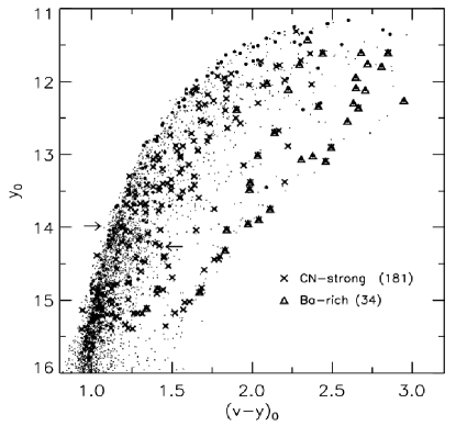
Figure 21.— Unreddened $y,\hbox{\it v--y\/}$ CMD of bright RGs. Objects in common with VL07 are plotted as filled circles. The crosses mark candidate CN-strong stars ($\delta CN>0.2$, see text for more details), while the triangles the $Ba$-rich stars according to the selection by VL07. The two arrows display the region covered by RG bump stars.

In passing we note that CN-strong stars are distributed over the entire magnitude range covered by our RG sample (Fig. 20). In particular, they are present above, below and through the RG bump region (horizontal arrows in Fig. 21). This further supports the evidence that these objects are related to MS and SGB stars apparently having enhancements in either C or N. Finally, Fig. 21 shows the barium-rich stars according to the selection by VL07. The clear correlation of these objects with the metal-rich RG stars located along the $\,\omega$ 3  branch strongly supports the recent findings by McDonald et al. (2008).

9.2. $\alpha$-element abundances

We took advantage of the accurate $\alpha$-element (O, Mg, Si, Ca, Ti) measurements of RG stars in $\omega$ Cen provided by ND95 (filled circles) and by PA02 (open circles) to investigate whether the photometric metallicities correlate with the abundance of these elements. We performed several tests and found that metallicities based on the $m_{0},(\hbox{\it v--y\/})_{0}$ and $m_{0},(\hbox{\it u--y\/})_{0}$ relations show very well defined correlations with the abundance of [Ca+Si/H]. Data plotted in Fig. 22 show that for metal abundances ranging from $\hbox{\rm[Fe/H]}\sim-1.6$ up to Solar metallicity they display a tight correlation. This correlation does not apply to more metal-poor objects, and indeed for [Ca+Si/H]$\approx$–1.5 and $\hbox{\rm[Fe/H]}\lesssim-1.7$ dex they form a plateau.

Figure 22.— [Ca+Si/H] spectroscopic abundances for RG stars in common with ND95 (filled circles) and PA02 (open circles) as a function of photometric metallicities based on the $m_{0},(\hbox{\it v--y\/})_{0}$ (top), and $m_{0},(\hbox{\it u--y\/})_{0}$ (bottom) semi-empirical MIC relations. The dashed lines display the bisector lines. Crosses mark CN-strong stars, the asterisk the CH-star and the plus the candidate CN-strong star ROA 248. The error bars account for both photometric and spectroscopic errors.

A good fraction of candidate CN-strong stars follows the same correlation, while the CH-star (asterisk) appears heavily depleted in Ca+Si abundance. A more detailed analysis concerning the possible occurrence of stars showing either a C,N and/or an $\alpha$-element enhancement or a large CH line blocking would require a larger sample of stars with accurate individual elemental abundances. Note that the correlation between the $\alpha$-elements and photometric metallicities might open new opportunities to discriminate between field and cluster RGs.

10. Summary and conclusions

We have presented new and accurate multiband Strömgren ($u,v,b,y$) and NIR ($J,H,K$) photometry of the Galactic Globular cluster $\omega$ Cen. On the basis of the new data sets we addressed several questions concerning the properties of the sub-populations present in this stellar system. The main findings are the following:

a) New calibrations of the $m_{0},(\hbox{\it b--y\/})_{0}$ MIC relation. We have provided new empirical and semi-empirical calibrations of $m_{0},(\hbox{\it b--y\/})_{0}$ MIC relations. Photometric metallicities based on the new MIC relations agree quite well with spectroscopic data and with photometric metallicities based on similar MIC relations available in the literature.

b) Comparison between photometric and spectroscopic iron abundances. We performed a detailed comparison between photometric and spectroscopic iron abundances. We selected iron abundances based on high-resolution spectra collected by ND95 (39), P02 (8) and J08 (118). We found, using four different MIC relations, that the mean difference between photometric and spectroscopic (ND95, P02) abundances is $<\Delta\hbox{\rm[Fe/H]}>\equiv\hbox{\rm[Fe/H]}_{phot}-\hbox{\rm[Fe/H]}_{spec}=0.17\pm 0.01$ with a dispersion in the residuals of $\sigma$=0.31 dex (47 stars). If we discard the RG stars affected by abundance anomalies in CN or CH, the mean difference becomes $<\Delta\hbox{\rm[Fe/H]}>=$$0.02\pm 0.02$ and the dispersion decreases by a factor of two ($\sigma$=0.16 dex, 36 stars). The same conclusion applies if we use the spectroscopic sample by J08: the difference is $<\Delta\hbox{\rm[Fe/H]}>=0.05\pm 0.03$, with $\sigma=0.37\,$dex (118 stars). When we remove the RGs affected by abundance anomalies we find that the mean difference deecreases ($<\Delta\hbox{\rm[Fe/H]}>=0.02\pm 0.04$), while the dispersion in the residuals attains a similar value ($\sigma=0.37\,$dex, 93 stars). Note that measurements of the $S3839$ index are available for only a small fraction of the sample, but these suggest that photometric and spectroscopic abundances are, on average, minimally different. The dispersion of the residuals decreases once we remove all the RGs affected by abundance anomalies. These findings do not depend significantly on the adopted MIC relations, although the $m_{0},(\hbox{\it b--y\/})_{0}$ MIC relations do have, on average, larger dispersions.

c) Metallicity distributions based on different MIC relations. We have estimated the metallicity distribution using both empirical and semi-empirical MIC relations. The six distributions based on two independent calibrations have similar properties, in particular, they show four main peaks at $\hbox{\rm[Fe/H]}_{phot}=$ $-1.73\pm 0.08$, $-1.29\pm 0.03$, $-1.05\pm 0.02$, $-0.80\pm 0.04$, and three minor peaks at $-0.42\pm 0.12$, $-0.07\pm 0.08$ and $0.24\pm 0.13$ dex (where the uncertainties are standard errors in the centroid of each peak). The four main peaks agree quite well with low- (N96, SK96), medium-(H04, S05b) and high-resolution (J08) spectroscopic iron abundances and with previous photometric metallicities (HR00, S05a). Spectroscopic abundances also suggest the occurrence of metal-rich ($\hbox{\rm[Fe/H]}=-0.60\pm 0.15$) stars in $\omega$ Cen(ND95; P00; Pancino 2004). The stars belonging to the solar metallicity tail should be regarded with caution since they might be either CN-strong stars or field RGs.

d) Identification of sub–populations according to their metal content. We identified four different metallicity regimes. The weighted mean fraction of stars in the metal-poor ($\hbox{\rm[Fe/H]}\leq-1.49$) component is $\sim 39\pm 1$%, with a sharp cutoff for $\hbox{\rm[Fe/H]}\approx-2.0$ dex. In comparison, the weighted mean fraction of stars in the metal–intermediate ($-1.49<\hbox{\rm[Fe/H]}\leq-0.93$) component is $\sim 32\pm 1$%, while the fraction of metal-rich ($-0.95<\hbox{\rm[Fe/H]}\leq-0.15$) stars is $\sim 19\pm 4$%, and the solar metallicity stars ($\hbox{\rm[Fe/H]}\approx 0$) represent only a small fraction of the total ($\sim 8\pm 5$%). This last apparent sub-population lacks a firm spectroscopic confirmation.

The new mosaic cameras available at telescopes of the 4–8m class, and the increased sensitivity of new CCDs to short wavelengths combine to make medium-band photometry very promising for constraining the nature of any composite stellar population that may be found in globular clusters. The same conclusion applies equally well to more complex systems such as the Galactic bulge and nearby dwarf galaxies (Faria et al. 2007).

e) Abundance anomalies. We have cross-correlated our optical-NIR photometric catalog with the large spectroscopic catalog collected by VL07. Using the $S3839$ index (cyanogen band) defined by VL07 and $(y-K)_{0}$ we selected a sample of 181 candidate CN-strong stars with a CN excess of $\delta{\hbox{CN}}>0.2$. Taken at face value this selection would imply a fraction of CN-strong stars of the order of 50%. We provided an independent estimate of the fraction of CN-strong stars from the difference between the iron content based on the semi-empirical $m_{0},(\hbox{\it v--y\/})_{0}$ (more sensitive to the CN-band strength) and the semi-empirical $m_{0},(\hbox{\it u--y\/})_{0}$ relations. We found that the fraction of candidate CN-strong RGs ($\Delta\hbox{\rm[Fe/H]}>0.2$ dex) is of the order of $19\pm 1$%. This fraction agrees quite well with the fraction of SGB stars that, according to Stanford et al. (2007), display enhancements in either C ($\sim$ 17%) or N ($\sim$ 16%) (see their Table 4). If these enhancements are caused by binary interaction, as suggested by Stanford et al. (2007, and references therein), the current evidence would imply that $\omega$ Cen hosts a population of binary stars that is at least a factor of five larger than suggested by spectroscopy (Mayor et al. 1996) and a factor of two larger than the typical binary fraction believed to be present in most GCs (Davies et al. 2006).

We also found that photometric metallicities correlate with the [Ca+Si/H] abundance from $\hbox{\rm[Fe/H]}\sim$ –1.6 up to Solar metallicity. More metal-poor stars display a plateau at [Ca+Si/H]$\approx$–1.5 and $\hbox{\rm[Fe/H]}\lesssim$ –1.7 dex.

This investigation is just a step in the ongoing effort to improve the use of Stroemgren indices as measures of chemical content. This should certainly be refined as more discriminating data become available. Our results also suggest the potential power of simultaneous use of optical data collected with other medium-band photometric systems. The DDO system (McClure & van den Bergh 1968) with filters centered on the CN molecular band at $\lambda\sim 4215$ Å, on the G band near 4300 Å, and on the magnesium complex near 5160 Å appears particularly promising. The use of the $hk$ index (ATT98) to estimate the calcium abundance of cluster HB and RG stars should also be explored further.

Table 1Positional, photometric and structural parameters of the Galactic Globular Cluster $\omega$ Cen.

Parameter		Ref.
$\alpha$ (J2000)	13 26 45	1
$\delta$ (J2000)	-47 28 37	1
$M_{V}$ (mag)	-10.3	1
$r_{c}$ (arcmin)	$2.58$	2
$r_{t}$ (arcmin)	$44.8$	2
$e$	$0.15$	3
$\sigma_{V}$ (km s-1)	$15$	4
E(B-V)	$0.11\pm 0.02$	5
$(m-M)_{0}$ (mag)	$13.70\pm 0.12$	6
$\mu_{\alpha}\times cos\delta,\mu_{\delta}$ (mas/yr)	(-3.97, -4.38)	7
Position angle (Degree)	$100$	3

Table 2Strömgren data adopted in this investigation.

Field	Images	FoV	RA	DEC
LF	25$u$,28$v$,22$b$,30$y$	$13.7\times 13.7$	13 26 24	-47 28 12
FG-1	3$u,3v,3b,3y$	$13.7\times 13.7$	13 26 24	-47 28 12
FG-2	4$u,4v,4b,4y$	$13.7\times 13.7$	13 25 48	-47 38 24
MH-1	2$v,2b,2y$	$6.3\times 6.3$	13 26 57	-47 33 09
MH-2	3$v,3b,3y$	$6.3\times 6.3$	13 26 59	-47 38 50

Table 3Log of scientific CCD images of $\omega$ Cen collected by LF and by FG.

Frame	Date	HJD	ET	Filter	Seeing
(1)	(2)	(3)	(4)	(5)	(6)
LF run
dfsc0656	28-03-99	2451265.7938	450	y	1.32
dfsc0660	28-03-99	2451265.8398	2000	u	2.59
dfsc0661	28-03-99	2451265.8519	900	v	1.50
dfsc0662	28-03-99	2451265.8600	600	b	1.58
dfsc0663	28-03-99	2451265.8665	450	y	1.82

Table 4Log of scientific CCD images of $\omega$ Cen collected by MH.

Frame	Field	Date	HJD	ET	Filter	Seeing
(1)	(2)	(3)	(4)	(5)	(6)	(7)
MH 1993 run
om1y3	MH-1	13-05-93	2449120.6384	30	y	2.36
om1b3	MH-1	13-05-93	2449120.6427	60	b	2.57
om1v3	MH-1	13-05-93	2449120.6474	120	v	2.65
om2y3	MH-2	13-05-93	2449120.7222	30	y	2.05
om2b3	MH-2	13-05-93	2449120.7265	60	b	2.21

Table 5NIR photometric data adopted in this investigation.

Field	Images	FoV	RA	DEC
ISAAC_NE	8$NB\_1.21$, 24$NB\_2.19$	$2.5\times 2.5$	13 26 36	-47 27 31
SOFI_A	36$J$,55$K_{s}$	$4.9\times 4.9$	13 26 46	-47 28 36
SOFI_C	33$u$,55$K_{s}$	$4.9\times 4.9$	13 26 07	-47 24 25
SOFI_D	12$J$,20$K_{s}$	$4.9\times 4.9$	13 26 11	-47 34 52
SOFI_om11	1$J,1K_{s}$	$4.9\times 4.9$	13 27 08	-47 32 36

Table 6Log of scientific NIR CCD images of $\omega$ Cen.

Frame	Date	HJD	ET	Filter	Seeing
(1)	(2)	(3)	(4)	(5)	(6)
ISAAC_NE field
f1_219_01	2005-02-20	2453456.2889	66	NB_2.19	0.51
f1_219_02	2005-02-20	2453456.2851	66	NB_2.19	0.41
f1_219_03	2005-02-20	2453456.2839	66	NB_2.19	0.40
f1_219_04	2005-02-20	2453456.2801	66	NB_2.19	0.48
f1_219_05	2005-02-20	2453456.2789	66	NB_2.19	0.45

Table 7Set of Strömgren standard stars observed by FG.

Star	Date	Filter
(1)	(2)	(3)
HD112039	15-04-99	$u,v,b,y$
HD181720	15-04-99	$u,v,b,y$
HD167756	15-04-99	$u,v,b,y$
HD165896	15-04-99	$u,v,b,y$
HD165793	15-04-99	$u,v,b,y$

Table 8Log of standard stars of the reference photometric night.

Star	HJD	ET	Filter
(1)	(2)	(3)	(4)
HD119896	2451334.9467	7	y
HD119896	2451334.9471	15	b
HD119896	2451334.9475	25	v
HD119896	2451334.9480	70	u
HD119896	2451334.9895	7	y

Table 9Log of HD standard stars observed at different airmass values.

Star	Airmass	HJD	ET	Filter
(1)	(2)	(3)	(4)	(5)
HD119896	1.263	51334.9467	7	y
HD119896	1.262	51334.9471	15	b
HD119896	1.260	51334.9475	25	v
HD119896	1.258	51334.9480	70	u
HD119896	1.134	51334.9895	7	y
HD119896	1.133	51334.9898	15	b
HD119896	1.132	51334.9902	25	v
HD119896	1.132	51334.9908	70	u
HD119896	1.068	51335.0353	7	y
HD119896	1.068	51335.0357	15	b
HD119896	1.067	51335.0361	25	v
HD119896	1.065	51335.0366	70	u

Table 10Extinction coefficients estimated for the observing nights.

Date	$k_{u}$	$k_{v}$	$k_{b}$	$k_{y}$
(1)	(2)	(3)	(4)	(5)
15-04-99	0.230	0.130	0.074	0.064
16-04-99	0.350	0.308	0.187	0.127
19-04-99	0.522	0.309	0.185	0.145
22-04-99	0.412	0.273	0.162	0.120
06-06-99	0.604	0.403	0.270	0.176

Table 11Multilinear regression coefficients for the Strömgren MIC relations: $m=\alpha+\beta\cdot\hbox{\rm[Fe/H]}+\gamma\cdot CI+\delta\cdot(\hbox{\rm[Fe/H]}\cdot CI)+\epsilon\cdot CI^{2}+\zeta\cdot(\hbox{\rm[Fe/H]}\cdot CI^{2})$.

Relation	$\alpha$	$\beta$	$\gamma$	$\delta$	$\epsilon$	$\zeta$	$r$
(1)	(2)	(3)	(4)	(5)	(6)	(7)	(8)
Empirical based on selected GCs (see CA07)
$m_{0},(\hbox{\it b--y\/})_{0}$	-0.51	-0.17$\pm$0.04	1.66$\pm$0.20	0.56$\pm$0.13	-0.020$\pm$0.14	-0.003$\pm$0.090	1.00
$[m],(\hbox{\it b--y\/})_{0}$	-0.47	-0.15$\pm$0.05	1.90$\pm$0.21	0.53$\pm$0.13	0.001$\pm$0.14	0.004$\pm$0.090	1.00
Semi-empirical based on transformations by Clem et al. (2004)
$m_{0},(\hbox{\it b--y\/})_{0}$	-0.64	-0.22$\pm$0.06	2.04$\pm$0.30	0.71$\pm$0.18	-0.22$\pm$0.20	-0.10$\pm$0.12	0.99
$[m],(\hbox{\it b--y\/})_{0}$	-0.51	-0.16$\pm$0.06	2.01$\pm$0.26	0.57$\pm$0.16	0.003$\pm$0.18	0.003$\pm$0.110	0.99

Table 12Spectroscopic measurements from Rutledge et al. (1997) and photometric metallicity estimates for the GCs adopted to validate the MIC relations.

Relation	M92	NGC6397	M13	NGC6752	NGC288	NGC1851	NGC362	M71	NGC104
(1)	(2)	(3)	(4)	(5)	(6)	(7)	(8)	(9)	(10)
Spectroscopy
$\ldots$	-2.24 $\pm$0.10	-1.91$\pm$0.14	-1.65$\pm$0.06	-1.54$\pm$0.09	-1.40$\pm$0.12	-1.33$\pm$0.10	-1.27$\pm$0.07	-0.73 $\pm$0.05	-0.71$\pm$0.05
Empirical based on selected GCs
$m_{0},(\hbox{\it b--y\/})_{0}$	$\ldots$	-2.04$\pm$0.15	$\ldots$	-1.67$\pm$0.18	-1.30$\pm$0.11	$\ldots$	-1.24$\pm$0.30	-0.48$\pm$0.34	$\ldots$
$[m],(\hbox{\it b--y\/})_{0}$	$\ldots$	-2.02$\pm$0.15	$\ldots$	-1.67$\pm$0.16	-1.31$\pm$0.12	$\ldots$	-1.28$\pm$0.24	-0.55$\pm$0.32	$\ldots$
Semi-empirical based on transformations by Clem et al. (2004)
$m_{0},(\hbox{\it b--y\/})_{0}$	-2.11$\pm$0.17	-2.05$\pm$0.16	-1.79$\pm$0.11	-1.69$\pm$0.15	-1.32$\pm$0.11	-1.53$\pm$0.18	-1.27$\pm$0.25	-0.50$\pm$0.36	-0.48$\pm$0.38
$[m],(\hbox{\it b--y\/})_{0}$	-2.09$\pm$0.16	-2.05$\pm$0.15	-1.81$\pm$0.09	-1.72$\pm$0.15	-1.38$\pm$0.11	-1.55$\pm$0.18	-1.34$\pm$0.22	-0.65$\pm$0.31	-0.61$\pm$0.31

Table 13Peaks and sigmas of multigaussian fits to the RG metallicity distributions based on the different MIC relations.

Relation	MP	MI1	MI2	MR1	MR2	SM1	SM2
Empirical calibrations
$m_{0},(\hbox{\it u--y\/})_{0}$	-1.74/0.32	-1.26/0.09	-1.03/0.11	-0.81/0.11	-0.48/0.24	-0.07/0.21	0.32/0.09
$m_{0},(\hbox{\it v--y\/})_{0}$	-1.70/0.32	-1.29/0.10	-1.06/0.07	-0.79/0.29	-0.20/0.11	-0.02/0.02	0.16/0.22
$m_{0},(\hbox{\it b--y\/})_{0}$	-1.79/0.26	-1.30/0.15	-1.04/0.09	-0.79/0.16	-0.46/0.15	-0.06/0.21	0.35/0.10
$Average$	-1.72/0.31	-1.30/0.09	-1.09/0.09	-0.88/0.10	-0.61/0.22	-0.03/0.17	0.32/0.08
Semi-empirical calibrations
$m_{0},(\hbox{\it u--y\/})_{0}$	-1.70/0.25	-1.32/0.09	-1.10/0.09	-0.89/0.11	-0.55/0.15	-0.20/0.07	0.00/0.15
$m_{0},(\hbox{\it v--y\/})_{0}$	-1.59/0.28	-1.24/0.10	-1.03/0.10	-0.76/0.16	-0.33/0.22	0.05/0.08	0.33/0.13
$m_{0},(\hbox{\it b--y\/})_{0}$	-1.84/0.24	-1.33/0.20	-1.03/0.18	-0.79/0.19	-0.49/0.14	-0.10/0.17	0.31/0.11
$Average$	-1.69/0.26	-1.28/0.12	-1.07/0.10	-0.88/0.04	-0.71/0.26	-0.03/0.18	0.30/0.17
$Mean$	-1.73$\pm$0.08	-1.29$\pm$0.03	-1.05$\pm$0.03	-0.80$\pm$0.04	-0.42$\pm$0.13	-0.07$\pm$0.08	0.24$\pm$0.13

Table 14Relative fraction of $\omega$ Cen RGs in the selected metallicity groups.

Relation	MP	MI	MR	SM
Empirical calibrations
$m_{0},(\hbox{\it u--y\/})_{0}$	47$\pm$2	31$\pm$1	16$\pm$1	5$\pm$1
$m_{0},(\hbox{\it v--y\/})_{0}$	38$\pm$1	32$\pm$1	23$\pm$1	7$\pm$1
$m_{0},(\hbox{\it b--y\/})_{0}$	38$\pm$1	31$\pm$1	17$\pm$1	14$\pm$1
$Average$	40$\pm$1	31$\pm$1	20$\pm$1	9$\pm$1
Semi-empirical calibrations
$m_{0},(\hbox{\it u--y\/})_{0}$	48$\pm$2	33$\pm$1	16$\pm$1	3$\pm$1
$m_{0},(\hbox{\it v--y\/})_{0}$	36$\pm$1	34$\pm$1	25$\pm$1	7$\pm$1
$m_{0},(\hbox{\it b--y\/})_{0}$	36$\pm$1	33$\pm$1	17$\pm$1	14$\pm$1
$Average$	38$\pm$1	34$\pm$1	20$\pm$1	8$\pm$1
$Mean$	39$\pm$1	32$\pm$1	19$\pm$4	8$\pm$5

References

- Andersen et al. (1999) Andersen, M. I., Piirola, V., Andersen, J., Lindberg, B. 1999, in Astrophysics with the NOT, ed. H. Karttunen and V.P. Piikkio, (Tuorla, Finland), 23
- Anthony-Twarog & Twarog (1994) Anthony-Twarog, B.J., & Twarog, B.A. 1994, AJ, 107, 1577 (ATT94)
- Anthony-Twarog & Twarog (1998) Anthony-Twarog, B.J., & Twarog, B.A. 1998, AJ, 116, 1922 (ATT98)
- Anthony-Twarog & Twarog (2000) Anthony-Twarog, B.J., & Twarog, B.A. 2000, AJ, 120, 3111
- Bell & Gustafsson (1978) Bell, R.A., & Gustafsson, B. 1978, A&AS, 34, 229
- Bessell & Brett (1988) Bessell, M. S., Brett, J. M. 1988, PASP, 100, 1134
- Bono et al. (2008) Bono, G., et al. 2008, ApJ, 686, L87
- Busso et al. (2001) Busso, M., Gallino, R., Lambert, D.L., Travaglio, C., & Smith, V.V. 2001, ApJ, 557, 802
- Calamida et al. (2005) Calamida, A. et al. 2005, AJ, 634, L69 (CA05)
- Calamida et al. (2007) Calamida, A. et al. 2007, ApJ, 670, 400 (CA07)
- (11) Calamida, A. et al. 2007b, in Mem. Soc. Astr. Italiana, Vol. 79, XXI Century Challenges for Stellar Evolution, ed. S. Cassisi and M. Salaris, 673 (CA07b)
- Calamida (2007) Calamida, A. 2007, PhD thesis, University of Rome Tor Vergata
- Cannon & Stobie (1973) Cannon, R.D., & Stobie, R.S. 1973, MNRAS, 162, 207
- Cardelli et al. (1989) Cardelli, J.A., Clayton, G.C., & Mathis, J.S. 1989, ApJ, 345, 245
- Carpenter (2001) Carpenter, J.M. 2001, AJ, 121, 2851
- Cassisi et al. (2004) Cassisi, S., Salaris, M., Castelli, F., & Pietrinferni, A. 2004, ApJ, 616, 498
- Castellani, Chieffi & Straniero (1990) Castellani, V., Chieffi, A., & Straniero, O. 1990, ApJS, 74, 463
- Castellani et al. (2006) Castellani, M., Castellani, V., Prada Moroni, P.G. 2006, A&A, 457, 569
- Castellani et al. (2007) Castellani, V., et al. 2007, ApJ, 663, 1021 (CAS07)
- Crawford & Barnes (1970) Crawford, D.L., & Barnes, J. V. 1970, AJ, 75,624
- Cunha et al. (2002) Cunha, K., Smith, V.V., Suntzeff, N.B., Norris, J.E., Da Costa, G.S., & Plez, B. 2002, AJ, 124, 379
- Clem et al. (2004) Clem, J. L., VandenBerg, Don A., Grundahl, F., & Bell, R. A. 2004, AJ, 127, 1227
- Del Principe et al. (2006) Del Principe, M., et al. 2006, ApJ, 77, 330
- Dickens & Wooley (1967) Dickens, R.J., & Wooley, R.v.d.R. 1967, , 128, 255
- Dickens & Bell (1976) Dickens, R.J., Bell, R.A. 1976, ApJ, 207, 506
- Faria et al. (2007) Faria, D., Feltzing, S., Lundstr m, I., Gilmore, G., Wahlgren, G. M., Ardeberg, A., Linde, P. 2007, A&A, 465, 357
- Freyhammer et al. (2005) Freyhammer, L. M., et al. 2005, ApJ, 623, 860
- Freeman & Rodgers (1975) Freeman, K.C., Rodgers, A.W. 1975, ApJ, 201, L71
- Gratton, Sneden & Carretta (2004) Gratton, R., Sneden, C., & Carretta, E. 2004, ARA&A, 42, 85
- Grundahl et al. (1998) Grundahl, F., Vandenberg, Don A., Andersen, M. I. 1998, ApJ, 500, 179
- Grundahl et al. (1999) Grundahl, F., Catelan, M., Landsman, W. B., Stetson, P. B., Andersen, M. I. 1999, ApJ, 524, 242
- Grundahl, Stetson, & Andersen (2002) Grundahl, F., Stetson, P. B., Andersen, M. I. 2002, A&A, 395, 481
- Harris (1996) Harris, W.E. 1996, AJ, 112, 1487
- Hilker et al. (2000) Hilker, M. 2000, A&A, 355, 994 (H00)
- Hilker & Richtler (2000) Hilker, M., & Richtler, T. 2000, A&A, 362, 895 (HR00)
- Hilker et al. (2004) Hilker, M., Kayser, A., Richtler, T., & Willemsen, P. 2004, A&A, 422, L9 (H04)
- Hughes & Wallerstein (2000) Hughes, J. & Wallerstein, G. 2000,AJ, 119, 1225
- Hughes et al. (2004) Hughes, J., Wallerstein, G., van Leeuwen, F., & Hilker, M. 2004, AJ, 127, 980
- Johnson et al. (2008) Johnson, C.I., Pilachowski, C.A., Simmerer, J., Schwenk, D. 2008, ApJ, 681, 1505 (J08)
- Kayser et al. (2006) Kayser, A., Hilker, M., Richtler, T., & Willemsen, P. G. 2006, A&A, 458, 777 (KA06)
- Krist (1995) Krist, J.E. 1995, in Hubble Space Telescope Workshop: Post Servicing Mission, ed. A. Koratkar & C. Leitherer (Baltimore: STScI), 311
- Lee et al. (1999) Lee, Y. W., Joo, J. M., Sohn, Y. J., et al. 1999, Nature, 402, 55
- Maeder & Meynet (2006) Maeder, A., & Meynet, G. 2006, A&A, 448, L37
- Mayor et al. (1996) Mayor, M., et al. 1996, in The origins, evolution, and destinies of binary stars in clusters, ed. E.F. Milone and J.-C. Mermilliod, (San Francisco: ASP), 190
- McClure & van den Bergh (1968) McClure, R.D., van den Bergh, S. 1968, AJ, 73, 313
- McDonald et al. (2008) McDonald, I., et al. 2008, MNRAS, 394, 831
- Mukherjee et al. (1992) Mukherjee, K., Anthony-Twarog, B.J., Twarog, B. A. 1992, PASP, 104, 561
- Norris et al. (1981) Norris, J.E., Cottrell, P.L., Freeman, K.C., Da Costa, G.S. 1981, ApJ, 244, 205
- Norris & Da Costa (1995) Norris, J.E., & Da Costa, G.S. 1995, ApJ, 447, 680 (ND95)
- Norris et al. (1996) Norris, J.E., Freeman, K.C., & Mighell, K.J. 1996, ApJ, 462, 241 (N96)
- Ochsenbein, Bauer & Marcout (2000) Ochsenbein, F., Bauer, P., & Marcout, J. 2000, A&AS, 143, 221
- O’Connor et al. (1998) O’Connor, J.A., Meaburn, J., & Bryce, M. 1998, MNRAS, 300, 411
- Olsen (1993) Olsen, E.H. 1993, A&AS, 102, 89 (O93)
- Pancino et al. (2000) Pancino, E., Ferraro, F.R., Bellazzini, M., Piotto, G., & Zoccali, M. 2000, ApJ, 534, 83 (PA00)
- Pancino et al. (2002) Pancino, E., Pasquini, L., Hill, V., Ferraro, F.R., & Bellazzini, M. 2002, ApJ, 568, L101 (PA02)
- Pancino (2004) Pancino, E., 2004, in Origin and Evolution of the Elements, ed. A. McWilliam and M. Rauch (Cambridge: Cambridge Univ. Press), 45
- Pietrinferni et al. (2006) Pietrinferni, A., Cassisi, S., Salaris, M. and Castelli, F. 2006, ApJ, 642, 697
- Reijns et al. (2006) Reijns, R.A., et al. 2006, A&A, 445, 503
- Rey et al. (2000) Rey, S.-C., et al. 2000, AJ, 119, 1824
- Rey et al. (2004) Rey, S.-C., Lee, Y.-W., Ree, C.H., Joo, J.-M., Sohn, Y.-J., Walker, A.R. 2004, AJ, 127, 958
- Richter et al. (1999) Richter, P., Hilker, M., & Richtler, T. 1999, A&A, 350, 476
- Rutledge et al. (1997) Rutledge, et al. 1997, PASP, 109, 907
- Schuster & Nissen (1988) Schuster, W. J., Nissen, P. E. 1988, A&AS, 221, 65 (SN88)
- Smith (1987) Smith, G.H. 1987, PASP, 99, 67
- Smith et al. (2000) Smith, V.V., et al. 2000, AJ, 119, 1239 (SM00)
- Sollima et al. (2004) Sollima, A., Ferraro, F. R., Origlia, L., Pancino, E., Bellazzini, M. 2004, A&A, 420, 173
- (67) Sollima, A., Ferraro, F.R., Pancino, E., Bellazzini, M. 2005a, MNRAS, 357, 265 (S05a)
- (68) Sollima, A., Pancino, E., Ferraro, F.R., Bellazzini, M., Straniero, O., & Pasquini, L. 2005b, AJ, 634, 332 (S05b)
- (69) Stanford, L., Da Costa, G.S., Norris, J.E. 2006, AJ, 647, 1075
- Stanford et al. (2007) Stanford, L.M., Da Costa, G.S., Norris, J.E., Cannon, R.D. 2007, ApJ, 667, 911
- Stetson (1987) Stetson, P. B. 1987, PASP, 99, 191
- Stetson (1991) Stetson, P. B. 1991, AJ, 102, 589
- Stetson (1994) Stetson, P. B. 1994, PASP, 106, 250
- Stetson (2000) Stetson, P. B. 2000, PASP, 112, 925
- Stetson et al. (2003) Stetson, P. B., Bruntt, H., & Grundahl, F. 2003, PASP, 115, 413
- Suntzeff & Kraft (1996) Suntzeff, N.B., & Kraft, R.P. 1996, AJ, 111, 1913 (SK96)
- Trager, King & Djorgovski (1995) Trager, S.C., King, I.R., & Djorgovski, S. 1995, AJ, 109, 218
- vandenBerg et al. (2000) VandenBerg, D. A., Swenson, F. J., Rogers, F. J., Iglesias, C. A., & Alexander, D. R. 2000, ApJ, 532, 430
- van de Ven et al. (2006) van de Ven, G., van den Bosch, R.C. E., Verolme, E.K., de Zeeuw, P.T. 2006, A&A, 445, 513
- van Leeuwen et al. (2000) van Leeuwen, F., Le Poole, R. S., Reijns, R. A., Freeman, K. C., & de Zeeuw, P. T. 2000, A&A, 360, 472 (LE00)
- van Loon et al. (2007) van Loon, J.T., van Leeuwen, F., Smalley, B., Smith, A.W., Lyons, N.A., McDonald, I., Boyer, M.L. 2007, MNRAS, 382, 1353 (VL07)
- Vanture et al. (2002) Vanture, A.D., Wallerstein, G., & Suntzeff, N.B. 2002, ApJ, 569, 984
- Villanova et al. (2007) Villanova, S., et al. 2007, ApJ, 663, 296
- Woolley (1966) Woolley, R.v.d.R. 1966, , 2, 1
- Zinn & West (1984) Zinn, R., & West, M. J. 1984, ApJS, 55, 45
- Zinn (1985) Zinn, R. 1985, ApJ, 293, 424