Dijet imbalance in hadronic collisions

Abstract

The imbalance of dijets produced in hadronic collisions has been used to extract the average transverse momentum of partons inside the hadrons. In this paper we discuss new contributions to the dijet imbalance that could complicate or even hamper this extraction. They are due to polarization of initial state partons inside unpolarized hadrons that can arise in the presence of nonzero parton transverse momentum. Transversely polarized quarks and linearly polarized gluons produce specific azimuthal dependences of the two jets that in principle are not suppressed. Their effects cannot be isolated just by looking at the angular deviation from the back-to-back situation, rather they enter jet broadening observables. In this way they directly affect the extraction of the average transverse momentum of unpolarized partons that is thought to be extracted. We discuss appropriately weighted cross sections to isolate the additional contributions.

I Introduction

Event shape observables have been widely studied for various reasons. In $e^{+}e^{-}$-annihilation, observables such as the thrust and jet broadening have been studied primarily to extract $\alpha_{s}(M_{z})$, cf. for instance Refs. Rakow:1981qn ; Catani:1992jc ; Dokshitzer:1998kz ; Jones:2003yv ; GehrmannDeRidder:2007hr ; Weinzierl:2009ms for theoretical studies and Refs. Berger:1983yp ; Naroska:1986si ; Acton:1993zh ; Abe:1994mf ; MovillaFernandez:1997fr ; Pfeifenschneider:1999rz ; Abdallah:2004xe ; Achard:2004sv ; Abbiendi:2005gb for experimental studies. In the center-of-mass system (cms) of the $e^{+}e^{-}$ collisions at lowest order in $\alpha_{s}$, the produced quark-antiquark pair is exactly back-to-back leading for two-jet events to a thrust $T$ equal to unity. Gluon radiation, i.e. order $\alpha_{s}$ corrections, gives rise to nonzero $1-T$ and also to nonzero jet broadening. In the perturbative regime these observables can be used to extract $\alpha_{s}$, which has been done recently at next-to-next-to-leading order Dissertori:2007xa ; Bethke:2008hf ; Dissertori:2009qa . The results compare very well with those obtained by other means of extraction. In the nonperturbative regime, hadronization will also lead to nonzero event or jet shapes. This is characterized by a mean transverse momentum $\langle k_{\perp}\rangle$, leading in general to a contribution suppressed by a power of the large scale, the cms energy $Q$. For example, in the nonperturbative regime $1-T\propto\langle k_{\perp}\rangle/Q$. It has been suggested that this contains universal information on $\alpha_{s}$ in the infrared regime. We refer to Ref. Dokshitzer:1998nz for a review on this topic.

Event and jet shapes have also been studied in hadronic collisions. Compared to $e^{+}e^{-}$-annihilation here the additional complication of initial parton transverse momenta arises. Another difference is that instead of the thrust axis, it is common to use the transverse thrust axis $n_{t}$, which is the axis in the transverse plane having maximum transverse energy flow. The corresponding transverse thrust is defined as Ellis:1986ig :

$$T_{t}=\max\sum_{i=1}^{n}\frac{|\boldsymbol{p}_{T}^{i}\cdot\boldsymbol{n}_{t}|}{E_{T}},$$ (1)

where $\boldsymbol{p}_{T}^{i}$ is the transverse momentum of the outgoing hadron $i$, $E_{T}=\sum_{i}|\boldsymbol{p}_{T}^{i}|$ is the total transverse energy (neglecting masses) and the transverse thrust axis is the transverse unit vector $\boldsymbol{n}_{t}$ that maximizes $T_{t}$. Here we use the notation of Ref. Ellis:1986ig , where also the jet broadening variable $Q_{t}$ is defined as:

$$Q_{t}=\sum_{i=1}^{n}|\boldsymbol{p}_{T}^{i}\times\boldsymbol{n}_{t}|.$$ (2)

An experimental investigation of the average $Q_{t}$ as a function of $E_{T}$ in $p\bar{p}$ collisions has been reported in Ref. Abe:1991dma . Higher order perturbative corrections to the transverse thrust and jet broadening are discussed in e.g. Refs. Nagy:2003tz ; Banfi:2004nk .

Assuming collinear factorization and ignoring broadening from hadronization, $Q_{t}$ will be zero for $2\to 2$ partonic subprocesses and only sensitive to $2\to 3$ processes, like for $e^{+}e^{-}$-annihilation except that there are more subprocesses to consider in hadronic collisions. Extraction of $\alpha_{s}$ in hadronic collisions Ellis:1992qq ; Affolder:2001hn is however complicated due to the presence of parton transverse momenta and the transverse momentum distribution of hadrons inside the jet. The former effect one can minimize by considering events with at least three pronounced jets, which means considering only large values of $Q_{t}$, whereas the latter effect could be minimized by considering $Q_{t}$ for jets, instead of hadrons. In fact, the quantity $Q_{t}$ for two-jet events, where $i$ now denotes the $i$-th jet and $n=2$, has been used to study and extract the average parton transverse momentum. This has been done for instance in Refs. Angelis:1978uv ; Clark:1979vc ; Baier:1979tp ; Corcoran:1979kd ; Angelis:1980bs ; Begel:1999rc ; Levai:2005fa ; Adler:2006sc ; Morsch:2006pf ; Fai:2006pd . As can be seen from those results, the average parton transverse momentum extracted from the data increases with energy ($\sqrt{s}$) and is in general much too large to be attributable to “intrinsic” transverse momentum. This is a consequence of soft parton radiation, similar to what happens for the transverse momentum distribution of vector boson production in hadronic processes Altarelli:1977kt ; Parisi:1979se ; Collins:1984kg ; Altarelli:1984xd (see also the instructive discussion in Ref. Collins:1985kw ). Resummation of soft radiation effectively broadens the transverse momentum dependence of the parton distributions, increasingly so with increasing center of mass energy.

In this paper we point out that besides initial parton transverse momentum and soft parton radiation, there are additional contributions to $Q_{t}$, even for the simplest two-jet case. These are contributions due to the transverse polarization of quarks and the linear polarization of gluons inside the initial unpolarized hadrons. These contributions can arise for nonzero initial parton transverse momentum. We will show how these effects contribute to $Q_{t}$ and discuss that besides complicating the extraction of the average parton transverse momentum from $Q_{t}$, they may even hamper that extraction altogether depending on their magnitude.

In Ref. Ellis:1986ig collinear factorization was assumed, making the observable $\langle Q_{t}\rangle$ only sensitive to $2\to 3$ subprocesses. In reality collinear factorization is not always applicable, due to the partonic transverse momentum effects. In a simple picture of a Gaussian distribution of intrinsic parton momentum $p_{t}$, the average value $\langle p_{t}\rangle$ can be extracted from $\langle Q_{t}\rangle$, but in fact, no factorization theorem has been established for two-jet or two-hadron production in $pp$ or $p\bar{p}$ collisions for observables that are sensitive to parton transverse momenta. To make matters worse, in the framework of transverse momentum dependent parton distribution functions, nowadays commonly referred to as TMDs, it even seems that factorization cannot be established for this particular type of process when taking into account nontrivial effects of gauge links Bomhof:2006dp ; Pijlman:2006tq ; Collins:2007nk ; Collins:2007jp ; MuldersRogers09 . This would cast doubt on any conclusion drawn from $\langle Q_{t}\rangle$ in hadronic collisions, except for large $Q_{t}$ where collinear factorization can be applied. But even if factorization will work out in some as yet unknown way, the additional contributions from spin dependent TMDs may complicate matters considerably. Schematically this can be seen as follows.

Consider the process $h_{1}h_{2}\to j_{1}j_{2}X$, where $j_{i}$ stands for produced jet $i$. In the plane transverse to the collision axis, $\delta\phi$ denotes the deviation of the (azimuthal) angle between the two jets from $\pi$, i.e. $\delta\phi=\phi_{j_{1}}-\phi_{j_{2}}-\pi$. It is sometimes referred to as the dijet imbalance. Let us consider only $2\to 2$ subprocesses. In collinear factorization the $\delta\phi$ dependence of the cross section will then only receive a contribution at $\delta\phi=0$. Allowing for parton transverse momentum in the initial hadrons leads to a smearing of the $\delta\phi$ distribution. For the idealized case of equal jet transverse momenta (both equal to $E_{T}/2$) the differential cross section takes the form:

$$\frac{d\sigma}{dE_{T}d\delta\phi}=A(Q_{t}^{2})+B(Q_{t}^{2})Q_{t}^{2}+C(Q_{t}^{2})Q_{t}^{4}\,,$$ (3)

where $Q_{t}=E_{T}|\sin(\delta\phi/2)|$ is equal to the absolute value of the transverse momentum of the two-jet system. $A,B,C$ are functions of $Q_{t}^{2}$, which do not need to vanish at $Q_{t}^{2}=0$. The terms $B$ and $C$ appear from spin effects inside the initial hadrons $h_{i}$, for which expressions will be presented in this paper. In general these spin-dependent contributions are not suppressed by powers of $1/E_{T}$, also not when arising from polarized gluons as claimed in Ref. Lu:2008qu . A result for $B$ has recently been obtained in Lu:2008qu following a calculation similar to the one for $p\bar{p}\to\gamma jX$ presented in Boer:2007nd . This contribution arises from the quark TMD $h_{1}^{\perp\,q}$ Boer:1997nt , which represents the distribution of transversely polarized quarks inside an unpolarized hadron. The new result in this paper is the contribution from $h_{1}^{\perp\,g}$ Mulders:2000sh , the distribution of linearly polarized gluons inside an unpolarized hadron, which gives rise to $C$. Upon ignoring these spin effects, only the term $A$ remains and the average $Q_{t}$ value in that case will indeed be directly related to the average transverse momentum that is thought to be extracted in Refs. Angelis:1978uv ; Clark:1979vc ; Baier:1979tp ; Corcoran:1979kd ; Angelis:1980bs ; Begel:1999rc ; Levai:2005fa ; Adler:2006sc ; Morsch:2006pf ; Fai:2006pd . Our results in principle cast doubt on whether the actual value of $\langle k_{t}^{2}\rangle$ has been extracted in those cases. In practice, it all depends on the magnitude of $B$ and $C$. We will present a simple Gaussian model to illustrate the generic shape of the modification of the dijet imbalance distribution by $B$ and $C$ terms.

The paper is organized as follows. First we will present the calculation and expressions for the cross section in Eq. (3), assuming factorization in terms of transverse momentum dependent correlators and ignoring the possible effects from gauge links. We will actually discuss the more general case in which the two jet transverse momenta are not equal, but differ by a small amount w.r.t. $E_{T}$. In that case the angular dependence is more involved than given in Eq. (3), even upon expansion in the small transverse momentum difference of the two jets with respect to their sum. We will first express the cross section in terms of the individual jet momenta through their sum and difference (section II, in particular Eq. (16)) and subsequently in terms of the sum and difference of the lengths of the jet momenta in order to arrive at the dijet imbalance distribution expressed in more standard variables (section III, in particular Eq. (51)). In section IV we discuss angular-projected asymmetries, such as $\langle\cos\delta\phi\rangle$ and the ones that can be used to extract $B$ and $C$. After that we consider the consequences of nonzero $h_{1}^{\perp}$ functions for the jet broadening quantity $Q_{t}$, in particular for the averages $\langle Q_{t}\rangle$ and $\langle Q_{t}^{2}\rangle$. Finally (section VI) we briefly address the open issues of factorization (breaking) and color flow dependence upon inclusion of gauge links. We end with conclusions and two appendices, one on relations among various variables in the transverse plane and one on photon-jet production that completes the treatment given in Ref. Boer:2007nd .

II Theoretical framework: calculation of the cross section

We consider the process

$$h_{1}(P_{1}){+}h_{2}(P_{2})\,{\rightarrow}\,{\rm jet}(K_{1}){+}{\rm jet}(K_{2}){+}X\,,$$ (4)

where the four-momenta of the particles are given within brackets, and the jet-jet pair in the final state is almost back-to-back in the plane perpendicular to the direction of the incoming hadrons. Along the lines of Ref. Boer:2007nd , we will instead of collinear factorization consider a generalized factorization scheme taking into account partonic transverse momenta. We make a lightcone decomposition of the two incoming hadronic momenta in terms of the light-like Sudakov vectors $n_{+}$ and $n_{-}$, satisfying $n_{+}^{2}\,{=}\,n_{-}^{2}\,{=}\,0$ and $n_{+}{\cdot}n_{-}\,{=}\,1$:

$$P_{1}^{\mu}=P_{1}^{+}n_{+}^{\mu}+\frac{M_{1}^{2}}{2P_{1}^{+}}n_{-}^{\mu}\ ,\qquad\text{and}\qquad P_{2}^{\mu}=\frac{M_{2}^{2}}{2P_{2}^{-}}n_{+}^{\mu}+P_{2}^{-}n_{-}^{\mu}\ ~{}.$$ (5)

The partonic momenta ($p_{1}$, $p_{2}$) can be expressed in terms of the lightcone momentum fractions ($x_{1}$, $x_{2}$) and the intrinsic transverse momenta ($p_{1T}$, $p_{2T}$), as follows

$$p_{1}^{\mu}=x_{1}^{\phantom{+}}\!P_{1}^{+}n_{+}^{\mu}+\frac{p_{1}^{2}{+}\boldsymbol{p}_{1T}^{2}}{2x_{1}^{\phantom{+}}\!P_{1}^{+}}n_{-}^{\mu}+p_{1T}^{\mu}\ ,\qquad\text{and}\qquad p_{2}^{\mu}=\frac{p_{2}^{2}{+}\boldsymbol{p}_{2T}^{2}}{2x_{2}^{\phantom{-}}\!P_{2}^{-}}n_{+}^{\mu}+x_{2}^{\phantom{-}}\!P_{2}^{-}n_{-}^{\mu}+p_{2T}^{\mu}\ .$$ (6)

In general $n_{+}$ and $n_{-}$ will define the lightcone components of every vector $a$ as $a^{\pm}\equiv a\cdot n_{\mp}$, while perpendicular vectors $a_{\perp}$ will always refer to the components of $a$ orthogonal to both incoming hadronic momenta, $P_{1}$ and $P_{2}$. Therefore in Eq. (6), if we neglect hadron masses, $p_{1T}^{\mu}=p_{1\perp}^{\mu}$ and $p_{2T}^{\mu}=p_{2\perp}^{\mu}$. We denote with $s$ the total energy squared in the hadronic cms frame, $s=(P_{1}+P_{2})^{2}=E^{2}_{\rm cms}$, and with $\eta_{i}$ the pseudo-rapidities of the outgoing partons, i.e. $\eta_{i}\,{=}\,{-}\ln\big{(}\tan(\frac{1}{2}\theta_{i})\big{)}$, $\theta_{i}$ being the polar angles of the outgoing partons in the same frame. Finally, we introduce the partonic Mandelstam variables

$$\hat{s}=(p_{1}+p_{2})^{2},\qquad\hat{t}=(p_{1}-K_{1})^{2},\qquad\hat{u}=(p_{1}-K_{2})^{2},$$ (7)

which satisfy the relations

$$-\frac{\hat{t}}{\hat{s}}\equiv y=\frac{1}{e^{\eta_{1}-\eta_{2}}\,{+}\,1}~{},\qquad{\rm and}\qquad-\frac{\hat{u}}{\hat{s}}=1-y~{}.$$ (8)

Following Refs. Boer:2007nd and Bacchetta:2007sz we assume that at sufficiently high energies the hadronic cross section factorizes in a soft parton correlator for each observed hadron and a hard part:

$$d\sigma^{h_{1}h_{2}\rightarrow{\rm jet}\,{\rm jet}\,X} = \frac{1}{2s}\,\frac{d^{3}K_{1}}{(2\pi)^{3}\,2E_{1}}\frac{d^{3}K_{2}}{(2\pi)^{3}\,2E_{2}}{\int}dx_{1}\,d^{2}\boldsymbol{p}_{1T}\,dx_{2}\,d^{2}\boldsymbol{p}_{2T}\,(2\pi)^{4}\delta^{4}(p_{1}{+}p_{2}{-}K_{1}{-}K_{2})$$ (9)

$$\qquad\qquad\qquad\qquad\qquad\times\sum_{a{,}b{,}c{,}d}\ \Phi_{a}(x_{1}{,}\boldsymbol{p}_{1T})\otimes\Phi_{b}(x_{2}{,}\boldsymbol{p}_{2T})\otimes\,|H_{ab\rightarrow cd}(p_{1},p_{2},K_{1},K_{2})|^{2}\ .$$

This form assumes the simplest possible factorization omitting any gauge link dependence in the correlators, which can modify or even break the factorization (see section VI for a discussion of these open issues).

In Eq. (9) the sum runs over all the incoming and outgoing partons taking part in the reaction. The convolutions $\otimes$ indicate the appropriate traces over Dirac indices and $|H|^{2}$ is the hard partonic squared amplitude. The parton correlators are defined on the lightfront LF ($\xi{\cdot}n\,{\equiv}\,0$, with $n\equiv n_{-}$ for parton 1 and $n\equiv n_{+}$ for parton 2); they describe the hadron $\rightarrow$ parton transitions and can be parameterized in terms of transverse momentum dependent (TMD) distribution functions. In particular, the quark content of an unpolarized hadron is at leading twist (omitting gauge links) described by the correlator Boer:1997nt

$$\Phi_{q}(x{,}\boldsymbol{p}_{T})={\int}\frac{d(\xi{\cdot}P)\,d^{2}\xi_{T}}{(2\pi)^{3}}\ e^{ip\cdot\xi}\,\langle P|\,\overline{\psi}(0)\,\psi(\xi)\,|P\rangle\,\big{\rfloor}_{\text{LF}}=\frac{1}{2}\,\bigg{\{}\,f_{1}^{q}(x{,}\boldsymbol{p}_{T}^{2})\;\hbox to0.0pt{\hbox to7.80904pt{\hfil/\hfil}\hss}P+ih_{1}^{\perp\,q}(x{,}\boldsymbol{p}_{T}^{2})\;\frac{[\hbox to0.0pt{\hbox to5.03125pt{\hfil/\hfil}\hss}p_{T},\hbox to0.0pt{\hbox to7.80904pt{\hfil/\hfil}\hss}P]}{2M}\bigg{\}}\,,$$ (10)

where $f_{1}^{q}(x,\boldsymbol{p}_{T}^{2})$ is the unpolarized quark distribution, which integrated over $\boldsymbol{p}_{T}$ gives the familiar lightcone momentum distribution $f_{1}^{q}(x)$. The time-reversal (T) odd function $h_{1}^{\perp q}(x,\boldsymbol{p}_{T}^{2})$ is interpreted as the quark transverse spin distribution in an unpolarized hadron Boer:1997nt . Analogously, for an antiquark,

$$\bar{\Phi}_{q}(x{,}\boldsymbol{p}_{T})=-{\int}\frac{d(\xi{\cdot}P)\,d^{2}\xi_{T}}{(2\pi)^{3}}\ e^{-ip\cdot\xi}\,\langle P|\,\overline{\psi}(0)\,\psi(\xi)\,|P\rangle\,\big{\rfloor}_{\text{LF}}=\frac{1}{2}\,\bigg{\{}\,f_{1}^{\bar{q}}(x{,}\boldsymbol{p}_{T}^{2})\;\hbox to0.0pt{\hbox to7.80904pt{\hfil/\hfil}\hss}P+ih_{1}^{\perp\,\bar{q}}(x{,}\boldsymbol{p}_{T}^{2})\;\frac{[\hbox to0.0pt{\hbox to5.03125pt{\hfil/\hfil}\hss}p_{T},\hbox to0.0pt{\hbox to7.80904pt{\hfil/\hfil}\hss}P]}{2M}\bigg{\}}\,.$$ (11)

The gluon correlator (omitting gauge links) is given by Mulders:2000sh

$$\Phi_{g}^{\mu\nu}(x{,}\boldsymbol{p}_{T}) = \frac{n_{\rho}\,n_{\sigma}}{(p{\cdot}n)^{2}}{\int}\frac{d(\xi{\cdot}P)\,d^{2}\xi_{T}}{(2\pi)^{3}}\ e^{ip\cdot\xi}\,\langle P|\,\operatorname{Tr}\big{[}\,F^{\mu\rho}(0)\,F^{\nu\sigma}(\xi)\,\big{]}\,|P\rangle\,\big{\rfloor}_{\text{LF}}$$ (12)

$$= \frac{1}{2x}\,\bigg{\{}-g_{T}^{\mu\nu}\,f_{1}^{g}(x{,}\boldsymbol{p}_{T}^{2})+\bigg{(}\frac{p_{T}^{\mu}p_{T}^{\nu}}{M^{2}}\,{+}\,g_{T}^{\mu\nu}\frac{\boldsymbol{p}_{T}^{2}}{2M^{2}}\bigg{)}\;h_{1}^{\perp\,g}(x{,}\boldsymbol{p}_{T}^{2})\bigg{\}}\,,$$

with $g^{\mu\nu}_{T}$ being a transverse tensor defined as

$$g^{\mu\nu}_{T}=g^{\mu\nu}-n_{+}^{\mu}n_{-}^{\nu}-n_{-}^{\mu}n_{+}^{\nu}\,.$$ (13)

The function $f_{1}^{g}(x{,}\boldsymbol{p}_{T}^{2})$ represents the unpolarized gluon distribution, while the T-even function $h_{1}^{\perp\,g}(x{,}\boldsymbol{p}_{T}^{2})$ is the distribution of linearly polarized gluons in an unpolarized hadron.

In order to derive an expression for the cross section in terms of parton distributions, we insert the parametrizations in Eqs. (10), (11) and (12) of the TMD correlators into Eq. (9). Furthermore, utilizing the decompositions of the parton momenta in Eq. (6), the $\delta$-function in Eq. (9) can be rewritten as

$$\delta^{4}(p_{1}{+}p_{2}{-}K_{1}{-}K_{2}) = \frac{2}{s}\,\delta\bigg{(}\,x_{1}{-}\frac{1}{\sqrt{s}}(\,|\boldsymbol{K}_{1\perp}|\,e^{\eta_{1}}\,{+}|\boldsymbol{K}_{2\perp}|\,e^{\eta_{2}}\,)\,\bigg{)}\,\delta\bigg{(}\,x_{2}{-}\frac{1}{\sqrt{s}}(\,|\boldsymbol{K}_{1\perp}|e^{-\eta_{1}}\,{+}|\boldsymbol{K}_{2\perp}|\,e^{-\eta_{2}}\,)\,\bigg{)}$$ (14)

$$\mspace{200.0mu}\times\delta^{2}(\boldsymbol{p}_{1T}{+}\boldsymbol{p}_{2T}{-}\boldsymbol{K}_{1\perp}{-}\boldsymbol{K}_{2\perp})\ ,$$

with corrections of order $\mathcal{O}(1/s)$. After integration over $x_{1}$ and $x_{2}$, from the first two $\delta$-functions on the r.h.s. of Eq. (14), one obtains

$$x_{1}=\frac{1}{\sqrt{s}}\bigg{(}\,|\boldsymbol{K}_{1\perp}|\,e^{\eta_{1}}\,{+}|\boldsymbol{K}_{2\perp}|\,e^{\eta_{2}}\,\bigg{)},\,\quad x_{2}{=}\frac{1}{\sqrt{s}}\bigg{(}\,|\boldsymbol{K}_{1\perp}|e^{-\eta_{1}}\,{+}|\boldsymbol{K}_{2\perp}|\,e^{-\eta_{2}}\,\bigg{)}\,,$$ (15)

which relates the partonic momentum fractions $x_{1}$, $x_{2}$ to the rapidities and the transverse momenta of the jets. These basic tree-level relations will be used in our treatment. We will not consider several other effects that need to be accounted for in practice such as the actually used jet definition and higher order corrections that affect the above relations and cause additional smearing.

The hadronic cross section can be written in the form

$$\frac{d\sigma^{h_{1}h_{2}\rightarrow{\rm jet}\,{\rm jet}\,X}}{d\eta_{1}d\eta_{2}d^{2}\boldsymbol{K}_{1\perp}d^{2}\boldsymbol{K}_{2\perp}}=\frac{\alpha_{s}^{2}}{s\boldsymbol{K}_{\perp}^{2}}\bigg{[}A(\boldsymbol{q}_{T}^{2})+B(\boldsymbol{q}_{T}^{2})\boldsymbol{q}_{T}^{2}\cos 2(\phi_{T}-\phi_{\perp})+C(\boldsymbol{q}_{T}^{2})\boldsymbol{q}_{T}^{4}\cos 4(\phi_{T}-\phi_{\perp})\bigg{]}$$ (16)

where $\boldsymbol{q}_{T}\equiv\boldsymbol{K}_{1\perp}+\boldsymbol{K}_{2\perp}$ and $\boldsymbol{K}_{\perp}\equiv(\boldsymbol{K}_{1\perp}-\boldsymbol{K}_{2\perp})/2$. The sum momentum $\boldsymbol{q}_{T}$ is useful as an in principle accessible experimental observable momentum which in our calculations via the delta function in Eq. (14) is related to intrinsic transverse momenta, $\boldsymbol{q}_{T}=\boldsymbol{p}_{1T}+\boldsymbol{p}_{2T}$. We denote with $\phi_{T}$ and $\phi_{\perp}$ the azimuthal angles of $\boldsymbol{q}_{T}$ and $\boldsymbol{K}_{\perp}$, respectively. Besides $\boldsymbol{q}_{T}^{2}$, the terms $A$, $B$ and $C$ depend on other kinematic variables often not explicitly indicated, namely $y$, $x_{1}$, $x_{2}$, and contain convolutions of the various parton distributions. These are discussed separately in the following three subsections, where explicit expressions for them can be found, calculated at leading order (LO) in perturbative QCD. In deriving these expressions we will often employ the approximation $|\boldsymbol{q}_{T}|\ll|\boldsymbol{K}_{1\perp}|\approx|\boldsymbol{K}_{2\perp}|\approx|\boldsymbol{K}_{\perp}|$ which is applicable in the situation in which the two jets are almost back-to-back in the transverse plane. However, in deriving Eq. (16) we must be particularly careful with the angular dependence, because approximations in the angular dependence that boil down to approximating $\phi_{1}\approx\phi_{2}+\pi$ (such as in Eq. (21) of Ref. Boer:2007nd ) will of course not give the proper dependence of the dijet imbalance angle $\delta\phi=\phi_{1}-\phi_{2}+\pi$. In Eq. (16) the combination $\phi_{T}-\phi_{\perp}$ appears, which will allow to isolate the terms $B$ and $C$ by $\boldsymbol{q}_{T}^{2}$-weighted integration over $\boldsymbol{q}_{T}$ (cf. section IV). However, in order to arrive at the $\delta\phi$ distribution discussed in the introduction, it is more convenient to express the cross section in terms of the combination $\phi_{T}-\phi_{j}$, where $\phi_{j}$ is the average jet direction angle, i.e. $\phi_{j}=(\phi_{1}+\phi_{2}-\pi)/2$ with $\phi_{1}$ and $\phi_{2}$ the azimuthal angles of the two outgoing jets in the transverse plane. In the present case where $|\boldsymbol{K}_{\perp}|\gg(|\boldsymbol{K}_{1\perp}|-|\boldsymbol{K}_{2\perp}|$), it holds that $\phi_{\perp}\approx\phi_{j}$ allowing the two angles to be identified to good approximation for all values of $\delta\phi$ (cf. Eq. (85)). In the limiting case when $|\boldsymbol{K}_{1\perp}|=|\boldsymbol{K}_{2\perp}|$, the angles $\phi_{\perp}$ and $\phi_{j}$ exactly coincide and the $T$ and $\perp$ directions are orthogonal, so we have exactly $\cos 2(\phi_{T}-\phi_{\perp})=-1$ (note that this will lead to Eq. (3) with a minus sign in front of $B$, but that is of course only a matter of definition) and $\cos 4(\phi_{T}-\phi_{\perp})=1$. This implies that all angular dependence then resides in $\boldsymbol{q}_{T}^{2}$, which is in that case solely depends on the off-collinearity of the jets through the dijet imbalance angle $\delta\phi$ (discussed in section III).

II.1 Angular independent part of the cross section

The term $A$ in Eq. (16) is the angular independent part of the cross section and is given by the sum of several contributions ${\cal A}^{ab\to cd}$ coming from the partonic subprocesses $ab\to cd$ underlying the reaction $h_{1}\,h_{2}\to{\rm jet}\,{\rm jet}\,X$:

$$A(y,x_{1},x_{2},\boldsymbol{q}_{T}^{2})=\sum_{a,b,c,d}{\cal A}^{ab\to cd}(y,x_{1},x_{2},\boldsymbol{q}_{T}^{2})\,,$$ (17)

with $a$,…, $d=q$, $q^{\prime}$, $\bar{q}$, $\bar{q}^{\prime}$, $g$. We denote with $q$ and $q^{\prime}$ two quarks having different flavors, and similar notation holds for the antiquarks. Furthermore, the following convolutions of unpolarized parton distributions are defined

$${\cal{F}}^{ab}(x_{1},x_{2},\boldsymbol{q}_{T}^{2}) \equiv \int d^{2}\boldsymbol{p}_{1T}\,d^{2}\boldsymbol{p}_{2T}\,\delta^{2}(\boldsymbol{p}_{1T}+\boldsymbol{p}_{2T}-\boldsymbol{q}_{T})f_{1}^{a}(x_{1},\boldsymbol{p}^{2}_{1T})f_{1}^{{b}}(x_{2},\boldsymbol{p}^{2}_{2T})\,,$$ (18)

where a sum over all (anti)quark flavors is understood. Our results for the terms ${\cal A}^{ab\to cd}$ in Eq. (17) are listed below, starting from the ones corresponding to the (anti)quark induced processes,

$${\cal A}^{qq^{\prime}\to qq^{\prime}} = a(y){\cal{F}}^{qq^{\prime}}(x_{1},x_{2},\boldsymbol{q}_{T}^{2})+a(1-y){\cal{F}}^{q^{\prime}q}(x_{1},x_{2},\boldsymbol{q}_{T}^{2})\,,$$ (19)

$${\cal A}^{q\bar{q}^{\prime}\to q\bar{q}^{\prime}} = a(y){\cal{F}}^{q\bar{q}^{\prime}}(x_{1},x_{2},\boldsymbol{q}_{T}^{2})+a(1-y){\cal{F}}^{\bar{q}^{\prime}q}(x_{1},x_{2},\boldsymbol{q}_{T}^{2})\,,$$ (20)

$${\cal A}^{qq\to qq} = \frac{N^{2}-1}{2N^{2}}\,y(1-y)\,\bigg{[}\frac{1+(1-y)^{2}}{y^{2}}+\frac{1+y^{2}}{(1-y)^{2}}-\frac{2}{N}\frac{1}{y(1-y)}\bigg{]}{\cal{F}}^{qq}(x_{1},x_{2},\boldsymbol{q}_{T}^{2})\,,$$ (21)

$${\cal A}^{q\bar{q}\to q\bar{q}} = b(y){\cal{F}}^{q\bar{q}}(x_{1},x_{2},\boldsymbol{q}_{T}^{2})+b(1-y){\cal{F}}^{\bar{q}q}(x_{1},x_{2},\boldsymbol{q}_{T}^{2})\,,$$ (22)

$${\cal A}^{q\bar{q}\to q^{\prime}\bar{q}^{\prime}} = \frac{N^{2}-1}{2N^{2}}\,y(1-y)\,\left[y^{2}+(1-y)^{2}\right]\bigg{[}{\cal{F}}^{q\bar{q}}(x_{1},x_{2},\boldsymbol{q}_{T}^{2})+{\cal{F}}^{\bar{q}q}(x_{1},x_{2},\boldsymbol{q}_{T}^{2})\bigg{]}\,,$$ (23)

$${\cal A}^{q\bar{q}\to gg} = \frac{N^{2}-1}{N}\bigg{(}y^{2}+(1-y)^{2}-\frac{1}{N^{2}}\bigg{)}\frac{y^{2}+(1-y)^{2}}{2}\bigg{[}{\cal{F}}^{q\bar{q}}(x_{1},x_{2},\boldsymbol{q}_{T}^{2})+{\cal{F}}^{\bar{q}q}(x_{1},x_{2},\boldsymbol{q}_{T}^{2})\bigg{]}\,,$$ (24)

with $N$ being the number of colors and

$$a(y) = \frac{N^{2}-1}{2N^{2}}\,(1-y)\frac{1+(1-y)^{2}}{y}\,,\qquad b(y)\,=\,a(y)+\frac{N^{2}-1}{2N^{2}}\,y(1-y)\,\bigg{[}y^{2}+(1-y)^{2}+\frac{2}{N}\frac{(1-y)^{2}}{y}\bigg{]}\,.$$ (25)

Analogously, from the gluon induced processes, one has:

$${\cal A}^{qg\to qg} = c(y){\cal{F}}^{qg}(x_{1},x_{2},\boldsymbol{q}_{T}^{2})+c(1-y){\cal{F}}^{gq}(x_{1},x_{2},\boldsymbol{q}_{T}^{2})\,,$$ (26)

$${\cal A}^{gg\to gg} = 4\,\frac{N^{2}}{N^{2}-1}\,\frac{(1-y(1-y))^{3}}{y(1-y)}{\cal{F}}^{gg}(x_{1},x_{2},\boldsymbol{q}_{T}^{2})\,,$$ (27)

$${\cal A}^{gg\to q\bar{q}} = \frac{N}{N^{2}-1}\,\bigg{(}y^{2}+(1-y)^{2}-\frac{1}{N^{2}}\bigg{)}\,\frac{y^{2}+(1-y)^{2}}{2}\,{\cal{F}}^{gg}(x_{1},x_{2},\boldsymbol{q}_{T}^{2})\,,$$ (28)

where

$$c(y)=\frac{1+(1-y)^{2}}{2}\,\bigg{[}\frac{1+(1-y)^{2}}{y}-\frac{y}{N^{2}}\bigg{]}~{}.$$ (29)

Agreement is found between the results given in the present subsection and the explicit expressions of the partonic cross sections published, for example, in Owens:1977sj ; Combridge:1977dm ; Cutler:1977qm ; Jaffe:1996ik ; Bomhof:2006ra . However, with respect to Ref. Lu:2008qu we find agreement with the expression for the unpolarized $qq$ production subprocess, but not for the $q\bar{q}$ production subprocesses. In particular, we find differences as compared with their Eqs. (24) and (33).

II.2 The $\cos 2(\phi_{T}-\phi_{\perp})$ angular distribution of the dijet

In Ref. Lu:2008qu it is shown that the subprocesses $qq\to qq$ and $q\bar{q}\to q\bar{q}$ contribute not only to the angular independent part of the cross section, according to Eqs. (21) and (22), but also to an azimuthal asymmetry of the dijet arising from the product of two T-odd functions, $h_{1}^{\perp q}h_{1}^{\perp q}$ or $h_{1}^{\perp q}h_{1}^{\perp\bar{q}}$. Such an asymmetry is similar to the one calculated in the Drell-Yan Boer:1999mm and in the photon-jet production Boer:2007nd processes. We refer to Boer:2007nd for the details of the derivation and present here only our final results. In analogy to Eq. (17), we write

$$B(y,x_{1},x_{2},\boldsymbol{q}_{T}^{2})=\sum_{a,b,c,d}{\cal B}^{ab\to cd}(y,x_{1},x_{2},\boldsymbol{q}_{T}^{2})\,,$$ (30)

with

$${\cal B}^{qq\to qq} = \frac{N^{2}-1}{N^{3}}\,y(1-y){\cal{H}}^{qq}(x_{1},x_{2},\boldsymbol{q}_{T}^{2})\,,$$ (31)

$${\cal B}^{q\bar{q}\to q\bar{q}} = d(y){\cal{H}}^{q\bar{q}}(x_{1},x_{2},\boldsymbol{q}_{T}^{2})+d(1-y){\cal{H}}^{\bar{q}q}(x_{1},x_{2},\boldsymbol{q}_{T}^{2})\,,$$ (32)

and

$$d(y) = \frac{N^{2}-1}{N^{3}}\,y(1-y)^{2}\,(1+Ny)~{}.$$ (33)

The following convolution of (transversely polarized) quark and antiquark distributions has been introduced

$$\boldsymbol{q}_{T}^{2}\,{\cal{H}}^{q\bar{q}}(x_{1},x_{2},\boldsymbol{q}_{T}^{2}) \equiv \frac{1}{M_{1}M_{2}}\sum_{\rm flavors}\int d^{2}\boldsymbol{p}_{1T}\,d^{2}\boldsymbol{p}_{2T}\,\delta^{2}(\boldsymbol{p}_{1T}+\boldsymbol{p}_{2T}-\boldsymbol{q}_{T})$$ (34)

$$\qquad\qquad\qquad\mbox{}\times\left(2(\boldsymbol{\hat{h}}\cdot\boldsymbol{p}_{1T})(\boldsymbol{\hat{h}}\cdot\boldsymbol{p}_{2T})-(\boldsymbol{p}_{1T}\cdot\boldsymbol{p}_{2T})\right)\ h_{1}^{\perp q}(x_{1},\boldsymbol{p}^{2}_{1T})h_{1}^{\perp\bar{q}}(x_{2},\boldsymbol{p}^{2}_{2T})\,,$$

with $\hat{\boldsymbol{h}}\equiv\boldsymbol{q}_{T}/|\boldsymbol{q}_{T}|$, and a similar definition holds for ${\cal H}^{qq}$ upon replacement of $\bar{q}\to q$ in Eq. (34). The small-$\boldsymbol{q}_{T}$ behavior of ${\cal H}$ is regular provided the integrations over $\boldsymbol{p}_{T}^{4}\,h_{1}^{\perp q}(x,\boldsymbol{p}_{T}^{2})$ converge. In addition to Eqs. (31) and (32), we find that the subprocesses $q\bar{q}\to gg$ and $q\bar{q}\to q^{\prime}\bar{q}^{\prime}$, not considered in Lu:2008qu , also show a $\cos 2(\phi_{T}-\phi_{\perp})$ angular dependence, leading respectively to

$${\cal B}^{q\bar{q}\to gg} = \frac{N^{2}-1}{N}\bigg{(}y^{2}+(1-y)^{2}-\frac{1}{N^{2}}\bigg{)}y(1-y)\bigg{[}{\cal{H}}^{q\bar{q}}(x_{1},x_{2},\boldsymbol{q}_{T}^{2})+{\cal{H}}^{\bar{q}q}(x_{1},x_{2},\boldsymbol{q}_{T}^{2})\bigg{]}\,,$$ (35)

and

$${\cal B}^{q\bar{q}\to q^{\prime}\bar{q}^{\prime}} = \frac{N^{2}-1}{N^{2}}\,y^{2}(1-y)^{2}\bigg{[}{\cal{H}}^{q\bar{q}}(x_{1},x_{2},\boldsymbol{q}_{T}^{2})+{\cal{H}}^{\bar{q}q}(x_{1},x_{2},\boldsymbol{q}_{T}^{2})\bigg{]}~{}.$$ (36)

Agreement is found between the results given in the present subsection and the explicit expressions of the polarized partonic cross sections published in Jaffe:1996ik ; Bomhof:2006ra ; Ji:1992ev ; Soffer:2002tf . For the polarized $qq$ production subprocess we find agreement with Ref. Lu:2008qu , but again not for the $q\bar{q}$ production subprocesses (in particular, we find a difference compared to their Eq. (26)).

II.3 The $\cos 4(\phi_{T}-\phi_{\perp})$ angular distribution of the dijet

The $\cos 4(\phi_{T}-\phi_{\perp})$ angular distribution of the dijet is related to the presence of linearly polarized gluons in unpolarized hadrons. This being a new result of the present paper, its derivation will be discussed in some more detail. The gluon-gluon induced part of the reaction under study, to lowest order in pQCD, is described in terms of the partonic two-to-two subprocesses

$$g(p_{1})+{g}(p_{2})\rightarrow g(K_{1})+g(K_{2})\,,\qquad{\rm and}\qquad g(p_{1})+{g}(p_{2})\rightarrow q(K_{1})+\bar{q}(K_{2})~{}.$$ (37)

The corresponding cross sections are given by

$$\frac{d\sigma^{gg\to gg}}{d\eta_{1}\,\,d\eta_{2}\,d^{2}\boldsymbol{K}_{\perp}\,d^{2}\boldsymbol{q}_{T}} = \frac{\alpha_{s}^{2}}{s\boldsymbol{K}_{\perp}^{2}}\bigg{[}{\cal A}^{gg\to gg}(y,x_{1},x_{2},\boldsymbol{q}_{T}^{2})+\int d^{2}\boldsymbol{p}_{1T}\,d^{2}\boldsymbol{p}_{2T}\,\delta^{2}(\boldsymbol{p}_{1T}+\boldsymbol{p}_{2T}-\boldsymbol{q}_{T})$$ (38)

$$\quad\times\frac{N^{2}}{N^{2}-1}\,y(1-y)(1-y(1-y))\,{\cal P}^{gg}(\boldsymbol{p}_{1T},\boldsymbol{p}_{2T},\boldsymbol{K}_{1\perp},\boldsymbol{K}_{2\perp})\bigg{]}\,,$$

and

$$\frac{d\sigma^{gg\to q\bar{q}}}{d\eta_{1}\,d\eta_{2}\,d^{2}\boldsymbol{K}_{\perp}\,d^{2}\boldsymbol{q}_{T}} = \frac{\alpha_{s}^{2}}{s\boldsymbol{K}_{\perp}^{2}}\,\bigg{[}{\cal A}^{gg\to q\bar{q}}(y,x_{1},x_{2},\boldsymbol{q}_{T}^{2})-\int d^{2}\boldsymbol{p}_{1T}\,d^{2}\boldsymbol{p}_{2T}\,\delta^{2}(\boldsymbol{p}_{1T}+\boldsymbol{p}_{2T}-\boldsymbol{q}_{T})$$ (39)

$$\quad\times\frac{N}{N^{2}-1}\,\frac{y(1-y)}{4}\,\bigg{(}y^{2}+(1-y)^{2}-\frac{1}{N^{2}}\bigg{)}\,{\cal{P}}^{gg}(\boldsymbol{p}_{1T},\boldsymbol{p}_{2T},\boldsymbol{K}_{1\perp},\boldsymbol{K}_{2\perp})\bigg{]}\,,$$

where

$${\cal{P}}^{gg}(\boldsymbol{p}_{1T},\boldsymbol{p}_{2T},\boldsymbol{K}_{1\perp},\boldsymbol{K}_{2\perp}) = \bigg{[}-\boldsymbol{p}_{1T}^{2}\boldsymbol{p}_{2T}^{2}+\frac{2}{\boldsymbol{K}_{\perp}^{4}}\,\bigg{(}(\boldsymbol{K}_{1\perp}\cdot\boldsymbol{K}_{2\perp})(\boldsymbol{p}_{1T}\cdot\boldsymbol{p}_{2T})-{(\boldsymbol{K}_{1\perp}\cdot\boldsymbol{p}_{1T})(\boldsymbol{K}_{2\perp}\cdot\boldsymbol{p}_{2T})}$$ (40)

$$~{}~{}~{}~{}~{}~{}-(\boldsymbol{K}_{1\perp}\cdot\boldsymbol{p}_{2T})(\boldsymbol{K}_{2\perp}\cdot\boldsymbol{p}_{1T})\bigg{)}^{2}\bigg{]}\frac{1}{M_{1}^{2}M_{2}^{2}}\,h_{1}^{\perp g}(x_{1},\boldsymbol{p}^{2}_{1T})\,h_{1}^{\perp g}(x_{2},\boldsymbol{p}^{2}_{2T})~{}.$$

The functions ${\cal A}^{gg\to gg}$ and ${\cal A}^{gg\to q\bar{q}}$, given in Eqs. (27) and (28), contain the convolution of unpolarized gluon distribution functions ${\cal F}^{gg}$ defined in Eq. (18). In order to show that the two cross sections in Eqs. (38) and (39) can be written in the same form as Eq. (16), we introduce the functions

$$\boldsymbol{q}_{T}^{4}\,{\cal{I}}^{gg}(x_{1},x_{2},\boldsymbol{q}_{T}^{2}) \equiv \frac{1}{M_{1}^{2}M_{2}^{2}}\int d^{2}\boldsymbol{p}_{1T}\,d^{2}\boldsymbol{p}_{2T}\,\delta^{2}(\boldsymbol{p}_{1T}+\boldsymbol{p}_{2T}-\boldsymbol{q}_{T})$$ (41)

$$\qquad\qquad\qquad\mbox{}\times\bigg{(}2(\hat{\boldsymbol{h}}\cdot\boldsymbol{p}_{1T})(\hat{\boldsymbol{h}}\cdot\boldsymbol{p}_{2T})-(\boldsymbol{p}_{1T}\cdot\boldsymbol{p}_{2T})\bigg{)}^{2}\ h_{1}^{\perp g}(x_{1},\boldsymbol{p}^{2}_{1T})h_{1}^{\perp g}(x_{2},\boldsymbol{p}^{2}_{2T})\,,$$

where again $\hat{\boldsymbol{h}}\equiv\boldsymbol{q}_{T}/|\boldsymbol{q}_{T}|$, and

$$\boldsymbol{q}_{T}^{4}\,{{\cal{L}}^{gg}(x_{1},x_{2},\boldsymbol{q}_{T}^{2})}\equiv\frac{1}{M_{1}^{2}M_{2}^{2}}\,\int d^{2}\boldsymbol{p}_{1T}\,d^{2}\boldsymbol{p}_{2T}\,\delta^{2}(\boldsymbol{p}_{1T}+\boldsymbol{p}_{2T}-\boldsymbol{q}_{T})\boldsymbol{p}^{2}_{1T}\boldsymbol{p}^{2}_{2T}h_{1}^{\perp g}(x_{1},\boldsymbol{p}^{2}_{1T})h_{1}^{\perp g}(x_{2},\boldsymbol{p}^{2}_{2T})~{}.$$ (42)

The small-$\boldsymbol{q}_{T}$ behavior of ${\cal I}$ and ${\cal L}$ are regular provided the integrations over $\boldsymbol{p}_{T}^{8}\,h_{1}^{\perp g}(x,\boldsymbol{p}_{T}^{2})$ converge. Hence we have

$$\int d^{2}\boldsymbol{p}_{1T}\,d^{2}\boldsymbol{p}_{2T}\,\delta^{2}(\boldsymbol{p}_{1T}+\boldsymbol{p}_{2T}-\boldsymbol{q}_{T}){\cal P}^{gg}$$

$$\qquad\mbox{}=\boldsymbol{q}_{T}^{4}\sum_{i,j,l,m=1}^{2}\,\frac{\boldsymbol{K}_{1\perp}^{\{i}\boldsymbol{K}_{2\perp}^{j\}}\boldsymbol{K}_{1\perp}^{\{l}\boldsymbol{K}_{2\perp}^{m\}}}{4\,\boldsymbol{K}_{\perp}^{4}}\bigg{[}2(\delta^{il}\delta^{jm}-\delta^{ij}\delta^{lm}+\delta^{im}\delta^{jl})({\cal{L}}^{gg}-{\cal{I}}^{gg})$$

$$\qquad\quad\mbox{}-\delta^{il}\delta^{jm}{\cal{L}}^{gg}+2\bigg{(}\frac{\boldsymbol{q}_{T}^{\{i}\boldsymbol{q}_{T}^{j\}}}{\boldsymbol{q}_{T}^{2}}-\delta^{ij}\bigg{)}\bigg{(}\frac{\boldsymbol{q}_{T}^{\{l}\boldsymbol{q}_{T}^{m\}}}{\boldsymbol{q}_{T}^{2}}-\delta^{lm}\bigg{)}(2{\cal{I}}^{gg}-{\cal{L}}^{gg})\bigg{]}$$

$$\qquad\mbox{}=\boldsymbol{q}_{T}^{4}\,\cos 2(2\phi_{T}-\phi_{1}-\phi_{2})(2{\cal I}^{gg}-{\cal L}^{gg})\,.$$ (43)

The difference between the angular dependence $\cos 2(2\phi_{T}-\phi_{1}-\phi_{2})=\cos 4(\phi_{T}-\phi_{j})$ and $\cos 4(\phi_{T}-\phi_{\perp})$ is of order $\boldsymbol{q}_{T}^{2}/\boldsymbol{K}_{\perp}^{2}$ (cf. Appendix A). Substituting Eq. (43) into Eqs. (38) and (39), and defining $d\sigma^{gg}\equiv d\sigma^{gg\to gg}+d\sigma^{gg\to q\bar{q}}$, we finally obtain

$$\frac{d\sigma^{gg}}{d\eta_{1}\,d\eta_{2}\,d^{2}\boldsymbol{K}_{\perp}\,d^{2}\boldsymbol{q}_{T}} = \frac{\alpha_{s}^{2}}{s\boldsymbol{K}_{\perp}^{2}}\bigg{[}{\cal A}^{gg}(y,x_{1},x_{2},\boldsymbol{q}_{T}^{2})+{\cal C}^{gg}(y,x_{1},x_{2},\boldsymbol{q}_{T}^{2})\,\boldsymbol{q}_{T}^{4}\,\cos 4(\phi_{T}-\phi_{\perp})\bigg{]}\,,$$

where ${\cal A}^{gg}\equiv{\cal A}^{gg\to gg}+{\cal A}^{gg\to q\bar{q}}$, ${\cal C}^{gg}\equiv{\cal C}^{gg\to gg}+{\cal C}^{gg\to q\bar{q}}$, with

$${\cal C}^{gg\to gg}=\frac{N^{2}}{N^{2}-1}\,y(1-y)(1-y(1-y))\,\bigg{[}2{\cal{I}}^{gg}(x_{1},x_{2},\boldsymbol{q}_{T}^{2})-{\cal{L}}^{gg}(x_{1},x_{2},\boldsymbol{q}_{T}^{2})\bigg{]}\,,$$ (45)

and

$${\cal C}^{gg\to q\bar{q}}=-\frac{N}{N^{2}-1}\,\frac{y(1-y)}{4}\,\bigg{(}y^{2}+(1-y)^{2}-\frac{1}{N^{2}}\bigg{)}\,\bigg{[}2{\cal{I}}^{gg}(x_{1},x_{2},\boldsymbol{q}_{T}^{2})-{\cal{L}}^{gg}(x_{1},x_{2},\boldsymbol{q}_{T}^{2})\bigg{]}~{}.$$ (46)

It turns out that the two subprocesses $gg\to gg$ and $gg\to q\bar{q}$ are the only ones that determine the $\cos 4(\phi_{T}-\phi_{\perp})$ dependence of the cross section. Therefore in Eq. (16)

$$C(y,x_{1},x_{2},\boldsymbol{q}_{T}^{2}) = {\cal C}^{gg}={\cal C}^{gg\to gg}+{\cal C}^{gg\to q\bar{q}}\,,$$ (47)

which, together with Eqs. (41)-(42) and Eqs. (45)-(46), leads to

$$C=\frac{N}{N^{2}-1}\,y(1-y)\bigg{[}N(1-y(1-y))-\frac{1}{4}\bigg{(}y^{2}+(1-y)^{2}-\frac{1}{N^{2}}\bigg{)}\bigg{]}\bigg{[}2{\cal I}^{gg}(x_{1},x_{2},\boldsymbol{q}_{T}^{2})-{\cal L}^{gg}(x_{1},x_{2},\boldsymbol{q}_{T}^{2})\bigg{]}\,,$$ (48)

showing how the azimuthal asymmetry under investigation is related to the T-even, spin and transverse momentum dependent parton distribution function $h_{1}^{\perp g}(x,\boldsymbol{p}_{T}^{2})$.

III Dijet imbalance distributions

In this section we study the cross section for the process $h_{1}\,h_{2}\to{\rm jet}\,{\rm jet}\,X$ in terms of the total transverse energy $E_{T}$ and the dijet imbalance $\delta\phi\equiv\phi_{1}-\phi_{2}-\pi$, which are the kinematic variables commonly used in the experiments. The dijet imbalance angle describes the deviation of the two jets from a back-to-back configuration (see Fig. 2 in Appendix A).

The transverse energy is the sum of the transverse energies of the two jets, $E_{T}=|\boldsymbol{K}_{1\perp}|+|\boldsymbol{K}_{2\perp}|$, and the difference is defined as $\Delta K_{\perp}=|\boldsymbol{K}_{1\perp}|-|\boldsymbol{K}_{2\perp}|$. In our basic expression for the cross section in Eq. (16) we have traded $\boldsymbol{K}_{1\perp}$ and $\boldsymbol{K}_{2\perp}$ for $\boldsymbol{q}_{T}$ and $\boldsymbol{K}_{\perp}$, but we can also trade the variables ($|\boldsymbol{K}_{1\perp}|$, $|\boldsymbol{K}_{2\perp}|$) for ($E_{T}$, $\Delta K_{\perp}$) and ($\phi_{1}$, $\phi_{2}$) for ($\phi_{j}$, $\delta\phi$). We find in the back-to-back approximation

$$\boldsymbol{q}_{T}^{2}=\Delta K_{\perp}^{2}\,\cos^{2}\left(\frac{\delta\phi}{2}\right)+E_{T}^{2}\sin^{2}\left(\frac{\delta\phi}{2}\right)\approx\Delta K_{\perp}^{2}+E_{T}^{2}\sin^{2}\left(\frac{\delta\phi}{2}\right)\,,$$ (49)

$$4\,\boldsymbol{K}_{\perp}^{2}=E_{T}^{2}\cos^{2}\left(\frac{\delta\phi}{2}\right)+\Delta K_{\perp}^{2}\,\sin^{2}\left(\frac{\delta\phi}{2}\right)\approx E_{T}^{2}\ .$$ (50)

In the first expression we cannot drop the term proportional to $\Delta K_{\perp}^{2}$ because it is not a good approximation for $\delta\phi\approx 0$, which is most relevant. Note also that this implies $\boldsymbol{q}_{T}^{2}\geq\Delta K_{\perp}^{2}$, i.e. $\Delta K_{\perp}^{2}$ sets a lower bound on the $\boldsymbol{q}_{T}^{2}$ values probed, which may be very relevant if the functions $A,B,C$ are steeply falling functions with increasing $\boldsymbol{q}_{T}^{2}$.

The cross section in Eq. (16) rewritten yields

$$\frac{d\sigma^{h_{1}h_{2}\rightarrow{\rm jet}\,{\rm jet}\,X}}{d\eta_{1}d\eta_{2}dE_{T}d\Delta K_{\perp}d\phi_{j}d\delta\phi}=\frac{\alpha_{s}^{2}}{2s}\bigg{[}A(\boldsymbol{q}_{T}^{2})+{B}(\boldsymbol{q}_{T}^{2})\,\boldsymbol{q}_{T}^{2}\,\cos 2(\phi_{T}-\phi_{j})+{C}(\boldsymbol{q}_{T}^{2})\,\boldsymbol{q}_{T}^{4}\,\cos 4(\phi_{T}-\phi_{j})\bigg{]}\,,$$ (51)

with $\boldsymbol{q}_{T}^{2}$ given in the unapproximated first part of Eq. (49) and

$$\boldsymbol{q}_{T}^{2}\,\cos 2(\phi_{T}-\phi_{j}) = \Delta K_{\perp}^{2}\,\cos^{2}\left(\frac{\delta\phi}{2}\right)-E_{T}^{2}\sin^{2}\left(\frac{\delta\phi}{2}\right)\,,$$ (52)

$$\boldsymbol{q}_{T}^{4}\,\cos 4(\phi_{T}-\phi_{j}) = \left[E_{T}^{2}\sin^{2}\left(\frac{\delta\phi}{2}\right)-\Delta K_{\perp}^{2}\,\cos^{2}\left(\frac{\delta\phi}{2}\right)\right]^{2}-E_{T}^{2}\,\Delta K_{\perp}^{2}\,\sin^{2}(\delta\phi)\,.$$ (53)

In this way we have arrived at an expression that is amenable to phenomenological studies, approximating $|\boldsymbol{K}_{1\perp}|\approx|\boldsymbol{K}_{2\perp}|\approx E_{T}/2$ only in places where the difference is negligible for all values of $\delta\phi$.

For $\Delta K_{\perp}=0$ we obtain:

$$\frac{d\sigma^{h_{1}h_{2}\rightarrow{\rm jet}\,{\rm jet}\,X}}{d\eta_{1}d\eta_{2}dE_{T}d\Delta K_{\perp}d\phi_{j}d\delta\phi}=\frac{\alpha_{s}^{2}}{2s}\bigg{[}A(\boldsymbol{q}_{T}^{2})-{B}(\boldsymbol{q}_{T}^{2})\boldsymbol{q}_{T}^{2}+{C}(\boldsymbol{q}_{T}^{2})\boldsymbol{q}_{T}^{4}\bigg{]}\,,$$ (54)

with in that case exactly $\boldsymbol{q}_{T}^{2}=E_{T}^{2}\sin^{2}\left(\delta\phi/2\right)$, and in essence recovering Eq. (3) (the sign in front of $B$ is just a matter of definition).

To illustrate the effect of nonzero $B$ and $C$ terms, we will make a Gaussian Ansatz for these functions of $\boldsymbol{q}_{T}^{2}$. We will take:

$$A(\boldsymbol{q}_{T}^{2})=\frac{R_{A}^{2}}{\pi}\exp(-\boldsymbol{q}_{T}^{2}R_{A}^{2}),\qquad B(\boldsymbol{q}_{T}^{2})=\frac{R_{B}^{4}}{c\pi}\exp(-\boldsymbol{q}_{T}^{2}R_{B}^{2}),\qquad C(\boldsymbol{q}_{T}^{2})=\frac{R_{C}^{6}}{2c^{2}\pi}\exp(-\boldsymbol{q}_{T}^{2}R_{C}^{2}),$$ (55)

normalized such that

$$\int d^{2}\boldsymbol{q}_{T}A(\boldsymbol{q}_{T}^{2})=1,\qquad\int d^{2}\boldsymbol{q}_{T}\boldsymbol{q}_{T}^{2}B(\boldsymbol{q}_{T}^{2})=1/c,\qquad\int d^{2}\boldsymbol{q}_{T}\boldsymbol{q}_{T}^{4}C(\boldsymbol{q}_{T}^{2})=1/c^{2}.$$ (56)

Fig. 1 shows a plot of the cross section in Eq. (51) as a function of $\delta\phi$ for the arbitrary, but perhaps realistic choices $|\boldsymbol{K}_{1\perp}|=30$ GeV, $|\boldsymbol{K}_{2\perp}|=31$ GeV, $R_{A}=0.5$ GeV^-2, $R_{B}=2R_{A},R_{C}=3R_{A}$ and $c=3$.

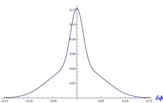
Figure 1: An illustration of the effect of sizeable $B$ and $C$ terms on the $\delta\phi$ distribution of the cross section in Eq. (51).

For smaller $\Delta K_{\perp}$ the shoulders become more pronounced, but already for $\Delta K_{\perp}=2$ GeV the shoulders are hardly distinguishable anymore. In general, $B$ and $C$ have to be significant in size and broad enough to generate an observable effect, i.e. for the $\delta\phi$ distribution to deviate visibly from a Gaussian distribution.

Although the $B$ and $C$ terms were not considered before in experimental analyses of dijet imbalance measurements in hadronic collisions, there is experimental data available that has some bearing on the size of $B$ compared to $A$. It comes from the measurement of the violation of the Lam-Tung relation in the Drell-Yan process. As shown in Ref. Boer:1999mm , this violation $\kappa$ is given by the ratio $\boldsymbol{q}_{T}^{2}\,{\cal{H}}^{q\bar{q}}/{\cal{F}}^{q\bar{q}}$ (Eq. (34) divided by the angular averaged result in Eq. (18)) but with the sums over flavors weighted with a factor $e_{q}^{2}$, the quark charge squared. This has the effect of emphasizing the contribution from up quarks. In the present two-jet production case, the ratio $\boldsymbol{q}_{T}^{2}\,B/A$ in the midrapidity region ($\eta_{1}\approx\eta_{2}\approx 0$) and for large $N$ can be approximated by $\boldsymbol{q}_{T}^{2}\,{\cal{H}}^{q\bar{q}}/{\cal{F}}^{q\bar{q}}$. The size of $\kappa$ in Drell-Yan may thus be expected to give some indication of the size of $\boldsymbol{q}_{T}^{2}\,B/A$. The violation of the Lam-Tung relation in Drell-Yan has recently been measured in $pp$ and $pd$ collisions Zhu:2008sj . It is consistent with no violation, but with sizeable errors. Small violation would be in line with the expectation that $h_{1}^{\perp}$ for antiquarks inside a proton is considerably smaller than for quarks. For $p\bar{p}$ one however expects a large violation, as observed in $\pi p$ collisions Falciano:1986wk ; Guanziroli:1987rp ; Conway:1989fs . So the effect of a nonzero $h_{1}^{\perp}$ for quarks may be mostly relevant for jet broadening studies in $p\bar{p}$ Abe:1991dma .

IV Weighted cross sections

Apart from the fact that nonzero $h_{1}^{\perp}$ functions for quarks and gluons modify the $\delta\phi$ distribution and hence affect the extraction of the average initial parton transverse momentum from this dijet imbalance distribution, it would in principle be of interest to extract these functions themselves from it. Therefore, the question arises whether one can project out the $B$ and $C$ terms separately. In Ref. Lu:2008qu this is discussed for $B$ only, but there are some problems with the proposed method. It was suggested that $\langle\cos\delta\phi\rangle$, i.e. the cross section integrated over $\delta\phi$ weighted with an additional factor of $\cos\delta\phi$, projects out a contribution from $h_{1}^{\perp\,q}$ exclusively. However, our result in Eq. (51) shows that $\langle\cos\delta\phi\rangle$ does not project out $B$ nor a part of $B$ exclusively, not even in the idealized case when $|\boldsymbol{K}_{1\perp}|=|\boldsymbol{K}_{2\perp}|$, as can be seen from Eq. (54). To see the appropriate weighting, we return to the form in Eq. (16) and note that $B$ is projected out by

$$\big{\langle}\cos 2(\phi_{T}-\phi_{\perp})\big{\rangle}\equiv\int\frac{d\phi_{T}}{2\pi}\ \cos 2(\phi_{T}-\phi_{\perp})\,{\frac{d\sigma^{h_{1}h_{2}\to{\rm jet}\,{\rm jet}\,X}}{d\eta_{1}\,d\eta_{2}\,d^{2}\boldsymbol{K}_{\perp}\,d^{2}\boldsymbol{q}_{T}}}=\frac{1}{2}\,\frac{\alpha_{s}^{2}}{s\boldsymbol{K}_{\perp}^{2}}\,\boldsymbol{q}_{T}^{2}\,B(y,x_{1},x_{2},\boldsymbol{q}_{T}^{2})~{}.$$ (57)

Integrating over the length of $\boldsymbol{q}_{T}$ gives with possible inclusion of additional weighting with powers of $\boldsymbol{q}_{T}^{2}$,

$$\pi\int d\boldsymbol{q}_{T}^{2}\ \ \left(\frac{\boldsymbol{q}_{T}^{2}}{M_{1}M_{2}}\right)^{M}\,\big{\langle}\cos 2(\phi_{T}-\phi_{\perp})\big{\rangle}=\int d^{2}\boldsymbol{q}_{T}\ \ \left(\frac{\boldsymbol{q}_{T}^{2}}{M_{1}M_{2}}\right)^{M}\,\cos 2(\phi_{T}-\phi_{\perp})\,{\frac{d\sigma^{h_{1}h_{2}\to{\rm jet}\,{\rm jet}\,X}}{d\eta_{1}\,d\eta_{2}\,d^{2}\boldsymbol{K}_{\perp}\,d^{2}\boldsymbol{q}_{T}}}\,,$$ (58)

in which we get for $M=1$ the factorized result

$$\pi\int d\boldsymbol{q}_{T}^{2}\ \left(\frac{\boldsymbol{q}_{T}^{2}}{M_{1}M_{2}}\right)\,\boldsymbol{q}_{T}^{2}\,{\cal{H}}^{qq}(x_{1},x_{2},\boldsymbol{q}_{T}^{2})=8\sum_{{\rm flavors}}\,h_{1}^{\perp q(1)}(x_{1})\,h_{1}^{\perp q(1)}(x_{2}),$$ (59)

in the $B$ contributions. For $M=0$, the expression does not deconvolute. In that case usable, but model dependent expressions may be obtained by making a Gaussian Ansatz for the transverse momentum shape of $h_{1}^{q}$. For the type of convolution that appears in $B$ this has been done in the literature, see for instance Ref. Boer:1997mf .

Next, we will analyze in some more detail the weighted asymmetry that projects out $C$. A measurement of the weighted cross section

$$\big{\langle}\cos 4(\phi_{T}-\phi_{\perp})\big{\rangle}\equiv\int\frac{d\phi_{T}}{2\pi}\ \cos 4(\phi_{T}-\phi_{\perp})\,{\frac{d\sigma^{h_{1}h_{2}\to{\rm jet}\,{\rm jet}\,X}}{d\eta_{1}\,d\eta_{2}\,d^{2}\boldsymbol{K}_{\perp}\,d^{2}\boldsymbol{q}_{T}}}=\frac{1}{2}\,\frac{\alpha_{s}^{2}}{s\boldsymbol{K}_{\perp}^{2}}\,\boldsymbol{q}_{T}^{4}\,C(y,x_{1},x_{2},\boldsymbol{q}_{T}^{2})\,,$$ (60)

with $C$ given in Eq. (48), would give access to the linearly polarized gluon distribution of a hadron. After integration over the length of $\boldsymbol{q}_{T}$ with possible inclusion of additional weighting with $\boldsymbol{q}_{T}^{2}$, we obtain

$$\pi\int d\boldsymbol{q}_{T}^{2}\ \ \left(\frac{\boldsymbol{q}_{T}^{2}}{M_{1}M_{2}}\right)^{M}\,\big{\langle}\cos 4(\phi_{T}-\phi_{\perp})\big{\rangle}=\int d^{2}\boldsymbol{q}_{T}\ \ \left(\frac{\boldsymbol{q}_{T}^{2}}{M_{1}M_{2}}\right)^{M}\,\cos 4(\phi_{T}-\phi_{\perp})\,{\frac{d\sigma^{h_{1}h_{2}\to{\rm jet}\,{\rm jet}\,X}}{d\eta_{1}\,d\eta_{2}\,d^{2}\boldsymbol{K}_{\perp}\,d^{2}\boldsymbol{q}_{T}}}\,.$$ (61)

In this case we get for $M=2$ the deconvoluted result

$$\pi\int d\boldsymbol{q}_{T}^{2}\ \left(\frac{\boldsymbol{q}_{T}^{2}}{M_{1}M_{2}}\right)^{2}\,\boldsymbol{q}_{T}^{4}\,\left(2\,{\cal I}^{gg}-{\cal L}^{gg}\right)=96\,h_{1}^{\perp g(2)}(x_{1})\,h_{1}^{\perp g(2)}(x_{2}),$$ (62)

in the $C$ contributions. In order to evaluate the integral in Eq. (60) without weights or study the explicitly $\boldsymbol{q}_{T}^{2}$-dependence, one can employ a Gaussian model for $h_{1}^{\perp g}$, of which the easiest choice has a factorized $x$ and $\boldsymbol{p}_{T}$ dependence, that is, neglecting the dependence on the factorization scale,

$$h_{1}^{\perp g}(x,\boldsymbol{p}_{T}^{2})=\frac{R_{h}^{2}}{\pi}\,h_{1}^{\perp g}(x)\,e^{-R_{h}^{2}\boldsymbol{p}_{T}^{2}}\,,$$ (63)

$$h_{1}^{\perp g(n)}(x)=\int d^{2}\boldsymbol{p}_{T}\,\left(\frac{\boldsymbol{p}_{T}^{2}}{2M^{2}}\right)^{n}\,h_{1}^{\perp g}(x,\boldsymbol{p}_{T}^{2})=\frac{n!}{(2\,M^{2}\,R_{h}^{2})^{n}}\,h_{1}^{\perp g}(x),$$ (64)

where $R_{h}$ is a size parameter related to the average partonic $\boldsymbol{p}_{T}^{2}$ by the relation $R_{h}^{2}=1/\langle\boldsymbol{p}_{T}^{2}\rangle$. For incoming (anti)protons, $R_{p}=R_{\bar{p}}\equiv R$, so one has

$$\int d^{2}\boldsymbol{q}_{T}\,\boldsymbol{q}_{T}^{4}\,(2{\cal I}^{gg}-{\cal L}^{gg}) = \frac{1}{M_{1}^{2}M_{2}^{2}}\int d^{2}\boldsymbol{q}_{T}\ d^{2}\boldsymbol{p}_{1T}\,d^{2}\boldsymbol{p}_{2T}\,\delta^{2}(\boldsymbol{p}_{1T}+\boldsymbol{p}_{2T}-\boldsymbol{q}_{T})\bigg{[}2\bigg{(}2(\hat{\boldsymbol{h}}\cdot\boldsymbol{p}_{1T})(\hat{\boldsymbol{h}}\cdot\boldsymbol{p}_{2T})-(\boldsymbol{p}_{1T}\cdot\boldsymbol{p}_{2T})\bigg{)}^{2}$$ (65)

$$\qquad\qquad-\boldsymbol{p}_{1T}^{2}\boldsymbol{p}_{2T}^{2}\bigg{]}\,\frac{R^{4}}{\pi^{2}}\,h_{1}^{\perp g}(x_{1})h_{1}^{\perp g}(x_{2})e^{-R^{2}(\boldsymbol{p}_{1T}^{2}+\boldsymbol{p}_{2T}^{2})}~{}.$$

Using the $\boldsymbol{p}_{2T}$ integration to eliminate the delta function in Eq. (65) and shifting the integration variable $\boldsymbol{p}_{1T}\to\boldsymbol{p}_{1T}^{\prime}=\boldsymbol{p}_{1T}-\frac{1}{2}\boldsymbol{q}_{T}$, one arrives at

$$\int d^{2}\boldsymbol{q}_{T}\,\boldsymbol{q}_{T}^{4}\,(2{\cal I}^{gg}-{\cal L}^{gg}) = \frac{1}{M_{1}^{2}M_{2}^{2}}\frac{R^{4}}{16\,\pi}\int d^{2}\boldsymbol{q}_{T}\,d\boldsymbol{p}_{1T}^{\prime 2}\,\boldsymbol{q}_{T}^{4}\,e^{-R^{2}\big{(}2\boldsymbol{p}_{1T}^{\prime 2}+\frac{1}{2}\boldsymbol{q}_{T}^{2}\big{)}}\,h_{1}^{\perp g}(x_{1})h_{1}^{\perp g}(x_{2})$$ (66)

$$= \frac{1}{2M_{1}^{2}M_{2}^{2}}\,\frac{1}{R^{4}}\,h_{1}^{\perp g}(x_{1})h_{1}^{\perp g}(x_{2})~{}.$$

Substituting Eq. (66) into Eq. (60) shows that for a Gaussian shape one finds for the unweighted average the final result

$$\pi\int d\boldsymbol{q}_{T}^{2}\ \langle\cos 4(\phi_{T}-\phi_{\perp})\rangle = \frac{\alpha_{s}^{2}}{s\boldsymbol{K}_{\perp}^{2}}\,\frac{N}{N^{2}-1}\,{y(1-y)}\bigg{[}N(1-y(1-y))-\frac{1}{4}\bigg{(}y^{2}+(1-y)^{2}-\frac{1}{N^{2}}\bigg{)}\bigg{]}$$ (67)

$$\qquad\qquad\qquad\mbox{}\times h_{1}^{\perp g(1)}(x_{1})h_{1}^{\perp g(1)}(x_{2}).$$

V Jet broadening

In our almost back-to-back jet situation, the jet-direction $j$ coincides with the transverse thrust axis and the jet broadening variable $Q_{t}$ defined in Eq. (2) is given by

$$Q_{t}=E_{T}\,\left|\sin\left(\frac{\delta\phi}{2}\right)\right|=|\boldsymbol{q}_{T}||\sin(\phi_{T}-\phi_{j})|\approx|\boldsymbol{q}_{T}||\sin(\phi_{T}-\phi_{\perp})|\,,$$ (68)

for which we refer to Eq. (83) in Appendix A and one needs to use Eqs. (84) and (85) to check the validity of the approximation. Using this expression we can now turn to the evaluation of the average jet broadening $\langle Q_{t}\rangle$ as a function of $|\boldsymbol{K}_{\perp}|$,

$$\langle Q_{t}\rangle\propto\int\frac{d\phi_{\perp}}{2\pi}\,d^{2}\boldsymbol{q}_{T}\ Q_{t}\left(|\boldsymbol{q}_{T}|,\phi_{T},\phi_{\perp}\right)\,\frac{d\sigma^{h_{1}h_{2}\rightarrow{\rm jet}\,{\rm jet}\,X}}{d^{2}\boldsymbol{K}_{\perp}\,d^{2}\boldsymbol{q}_{T}}~{}.$$ (69)

The differential cross section in the integrand is obtained from Eq. (16) and contains, besides the well-known, angular independent term $A$, also the terms $B$ (due to the transverse polarization of quarks and antiquarks in the colliding hadrons) and $C$ (related to the linear polarization of gluons). The following integrals,

$$\int_{0}^{2\pi}d\phi_{T}\,|\sin(\phi_{T}-\phi_{\perp})|=4\,,$$ (70)

$$\int_{0}^{2\pi}d\phi_{T}\,|\sin(\phi_{T}-\phi_{\perp})|\cos 2(\phi_{T}-\phi_{\perp})=-\frac{4}{3}\,,$$ (71)

$$\int_{0}^{2\pi}d\phi_{T}\,|\sin(\phi_{T}-\phi_{\perp})|\cos 4(\phi_{T}-\phi_{\perp})=-\frac{4}{15}\,$$ (72)

are all different from zero, meaning that the $A$, $B$ and $C$ terms contribute to $\langle Q_{t}\rangle$:

$$\langle Q_{t}\rangle\propto\int d^{2}\boldsymbol{q}_{T}|\boldsymbol{q}_{T}|\bigg{[}A(\boldsymbol{q}_{T}^{2})-\frac{1}{3}{B}(\boldsymbol{q}_{T}^{2})\boldsymbol{q}_{T}^{2}-\frac{1}{15}{C}(\boldsymbol{q}_{T}^{2})\boldsymbol{q}_{T}^{4}\bigg{]}~{}.$$ (73)

In order to calculate $\langle Q_{t}^{2}\rangle$, one needs to evaluate the integrals

$$\int_{0}^{2\pi}d\phi_{T}\,\sin^{2}(\phi_{T}-\phi_{\perp})=\pi\,,$$ (74)

$$\int_{0}^{2\pi}d\phi_{T}\,\sin^{2}(\phi_{T}-\phi_{\perp})\cos 2(\phi_{T}-\phi_{\perp})=-\frac{\pi}{2}\,,$$ (75)

$$\int_{0}^{2\pi}d\phi_{T}\,\sin^{2}(\phi_{T}-\phi_{\perp})\cos 4(\phi_{T}-\phi_{\perp})=0\,,$$ (76)

which show that only the terms $A$ and $B$ enter in the estimate of $\langle Q_{t}^{2}\rangle$:

$$\langle Q_{t}^{2}\rangle\propto\int d^{2}\boldsymbol{q}_{T}\boldsymbol{q}_{T}^{2}\bigg{[}A(\boldsymbol{q}_{T}^{2})-\frac{1}{2}{B}(\boldsymbol{q}_{T}^{2})\boldsymbol{q}_{T}^{2}\bigg{]}~{}.$$ (77)

VI Color flow dependence and factorization

In our treatment in this paper we have simply convoluted the quark and gluon correlators with the hard partonic cross sections, without worrying about possible nontrivial effects arising from the gauge link structure in these correlators. The proper gauge invariant definitions of TMDs as well as collinear correlators involve nonlocal operators containing path-ordered exponentials, the gauge links. The gauge link is the result of resumming all gluons with polarizations along the momentum of a particular hadron into the soft parts. In the case of TMDs the path of the gauge links generally depends on the process. The path dependence disappears after integration over transverse momenta. In the collinear correlators, one can usually choose a gauge that makes the gauge link unity, but the same procedure for TMDs can leave transverse pieces that are situated at lightcone infinity. These links can have physical effects, for instance in single transverse spin asymmetries that arise from the Sivers effect, which is described by a T-odd TMD. The Sivers asymmetries in semi-inclusive deep inelastic scattering and the Drell-Yan process are predicted to differ by a sign as a consequence of the gauge links Collins:2002kn .

In the more complicated processes $h_{1}^{\uparrow}h_{2}\rightarrow\gamma/{\rm jet}+{\rm jet}+X$ the single spin asymmetries involving the Sivers function Bacchetta:2007sz ; Boer:2003tx ; Bomhof:2007su come from correlators with more complex paths in the gauge links. This causes deviations that are more involved than a simple sign change with respect to e.g. semi-inclusive deep inelastic scattering. But also in this case, calculable process-dependent “color flow” factors can be obtained which may be different for each hard partonic subprocess. In this way they allow for the calculation of particular weighted cross sections in dijet production, resulting in a small asymmetry Bomhof:2007su ; Qiu:2007ey ; Vogelsang:2007jk , as also shown by the data Abelev:2007ii . However, claims of possible factorization breaking have been put forward for this process Collins:2007nk ; Collins:2007jp and this remains an open question.

For observables involving a product of two T-odd TMDs, such as the one discussed in the present paper, the situation is less clear. For $\cos 2\phi$ asymmetries in Drell-Yan Boer:1999mm and $h_{1}h_{2}\to\gamma\,{\rm jet}\,X$ the effects of nontrivial gauge links were included in Ref. Boer:2007nd following the methods outlined in Refs. Bomhof:2006dp ; Pijlman:2006tq ; Bomhof:2006ra ; Bomhof:2007xt . In both cases the color flow factor obtained was $+1$. However, since the methods used were developed for observables involving a single non-contracted transverse momentum $p_{T}$ for a T-odd TMD for one of the hadrons in the process, the extension to cases in which non-contracted transverse momenta of partons in two different hadrons are involved certainly needs careful study. The $p_{T}$-dependence for $h_{1}^{\perp}$ in the correlators for gluons, moreover, has a rank two tensor structure in the non-contracted transverse momentum, although it is T-even. For the present case of dijet production (for which nontrivial color flow factors were presented in Ref. Lu:2008qu ), which is necessarily more complicated and for which doubts about factorization have been put forward, at this stage we do not include any color flow factors. Since we have presented the expressions for each partonic subprocess separately, it is possible to include the correct factors at a later stage, once they have been firmly established. If factorization cannot be proven for the process of interest, however, this not only implies that the functions $h_{1}^{\perp}$ cannot be extracted but neither can in that case $\langle p_{T}^{2}\rangle$ be obtained.

VII Summary and Conclusions

In this paper we study the effects of transverse momenta of the initial state hadrons in hadronic dijet production. The transverse momentum produces an imbalance in the dijets in the transverse plane. In the usual treatments the effects are attributed to gluon radiation and to the transverse momentum dependence of the unpolarized quark distributions. We look at the effects of two additional TMD functions that enter in the scattering of unpolarized hadrons, the distribution of transversely polarized quarks ($h_{1}^{\perp q}$) and the distribution of linearly polarized gluons ($h_{1}^{\perp g}$). They produce specific azimuthal dependences of the two jets, that are not suppressed a priori. The effects cannot be isolated by only looking at the angular deviation from the back-to-back situation, but depend on the jet transverse energy and the contributions to it of the two jets. We have discussed appropriate weighting to isolate the specific additional contributions. We also pointed out their effect on the jet broadening quantities $\langle Q_{t}\rangle$ and $\langle Q_{t}^{2}\rangle$, which we considered for the simplest two-jet case, but the conclusion that $h_{1}^{\perp}$ functions contribute to them also affects the more general cases containing a sum over hadrons. This in principle complicates the extraction of the average initial parton transverse momentum from the jet broadening, but possibly even hampers it altogether if factorization of the (sufficiently sizeable) spin dependent contributions indeed turns out to be broken.

Appendix A Transverse plane variables

In the transverse plane we have the two jet momenta $\boldsymbol{K}_{1\perp}$ and $\boldsymbol{K}_{2\perp}$ defining azimuthal angles $\phi_{1}$ and $\phi_{2}$. From them one can construct the sum and difference angles,

$$\phi_{j}=(\phi_{1}+\phi_{2}-\pi)/2,$$ (78)

$$\delta\phi=\phi_{1}-\phi_{2}-\pi.$$ (79)

The sum and difference of the transverse energies of the two jets, $|\boldsymbol{K}_{1\perp}|$ and $|\boldsymbol{K}_{1\perp}|$, define

$$E_{T}=|\boldsymbol{K}_{1\perp}|+|\boldsymbol{K}_{2\perp}|$$ (80)

$$\Delta K_{\perp}=|\boldsymbol{K}_{1\perp}|-|\boldsymbol{K}_{2\perp}|$$ (81)

Figure 2: The transverse plane is defined as orthogonal with respect to the two incoming hadrons. The jet direction ($j$) is defined as $\phi_{j}=(\phi_{1}+\phi_{2}-\pi)/2$. The momenta $\boldsymbol{q}_{T}=\boldsymbol{K}_{1\perp}+\boldsymbol{K}_{2\perp}$ and $\boldsymbol{K}_{\perp}=(\boldsymbol{K}_{1\perp}-\boldsymbol{K}_{2\perp})/2$ define the azimuthal angles $\phi_{T}$ and $\phi_{\perp}$.

One can use $d^{2}\boldsymbol{K}_{1\perp}\,d^{2}\boldsymbol{K}_{2\perp}$ = $\tfrac{1}{8}\,(E_{T}^{2}-\Delta K_{\perp}^{2})\,dE_{T}\,d\Delta K_{\perp}\,d\phi_{j}\,d\delta\phi$ for the phase space or go to the sum and difference momenta and their angles as shown in Fig. 2. In that case one has $d^{2}\boldsymbol{K}_{1\perp}\,d^{2}\boldsymbol{K}_{2\perp}$ = $d^{2}\boldsymbol{K}_{\perp}\,d^{2}\boldsymbol{q}_{T}$ = $|\boldsymbol{q}_{T}|\,|\boldsymbol{K}_{\perp}|d|\boldsymbol{q}_{T}|\,d|\boldsymbol{K}_{\perp}|\,d\phi_{T}\,d\phi_{\perp}$. We have the following exact relations

$$|\boldsymbol{q}_{T}|\,\cos(\phi_{T}-\phi_{j})=\Delta K_{\perp}\,\cos(\delta\phi/2),$$ (82)

$$|\boldsymbol{q}_{T}|\,\sin(\phi_{T}-\phi_{j})=E_{T}\,\sin(\delta\phi/2),$$ (83)

$$2\,|\boldsymbol{K}_{\perp}|\,\cos(\phi_{\perp}-\phi_{j})=E_{T}\,\cos(\delta\phi/2),$$ (84)

$$2\,|\boldsymbol{K}_{\perp}|\,\sin(\phi_{\perp}-\phi_{j})=\Delta K_{\perp}\,\sin(\delta\phi/2),$$ (85)

$$\boldsymbol{q}_{T}^{2}=\Delta K_{\perp}^{2}\,\cos^{2}(\delta\phi/2)+E_{T}^{2}\,\sin^{2}(\delta\phi/2)=\Delta K_{\perp}^{2}+(E_{T}^{2}-\Delta K_{\perp}^{2})\,\sin^{2}(\delta\phi/2),$$ (86)

$$4\,\boldsymbol{K}_{\perp}^{2}=E_{T}^{2}\,\cos^{2}(\delta\phi/2)+\Delta K_{\perp}^{2}\,\sin^{2}(\delta\phi/2)=E_{T}^{2}-(E_{T}^{2}-\Delta K_{\perp}^{2})\,\sin^{2}(\delta\phi/2),$$ (87)

$$2|\boldsymbol{q}_{T}|\,|\boldsymbol{K}_{\perp}|\,\cos(\phi_{T}-\phi_{\perp})=E_{T}\,\Delta K_{\perp},$$ (88)

$$2|\boldsymbol{q}_{T}|\,|\boldsymbol{K}_{\perp}|\,\sin(\phi_{T}-\phi_{\perp})=(E_{T}^{2}-\Delta K_{\perp}^{2})/2\,\sin(\delta\phi).$$ (89)

We note that the order of the momenta is $|\boldsymbol{q}_{T}|\sim\Delta K_{\perp}\sim M$ (hadronic scale) while $E_{T}\sim 2\,|\boldsymbol{K}_{\perp}|\sim\sqrt{s}$, so we see from Eq. (83) that $\delta\phi\sim M/\sqrt{s}$ and from Eq. (85) that $\phi_{\perp}-\phi_{j}\sim M^{2}/s$. Further useful relations are

$$|\boldsymbol{q}_{T}|^{2}\,\cos 2(\phi_{T}-\phi_{\perp})\approx|\boldsymbol{q}_{T}|^{2}\,\cos 2(\phi_{T}-\phi_{j})=\Delta K_{\perp}^{2}\,\cos^{2}(\delta\phi/2)-E_{T}^{2}\,\sin^{2}(\delta\phi/2),$$ (90)

$$|\boldsymbol{q}_{T}|^{2}\,\sin 2(\phi_{T}-\phi_{\perp})\approx|\boldsymbol{q}_{T}|^{2}\,\sin 2(\phi_{T}-\phi_{j})=E_{T}\,\Delta K_{\perp}\,\sin(\delta\phi),$$ (91)

$$|\boldsymbol{q}_{T}|^{4}\,\cos 4(\phi_{T}-\phi_{\perp})\approx|\boldsymbol{q}_{T}|^{4}\,\cos 4(\phi_{T}-\phi_{j})\approx\Delta K_{\perp}^{4}+E_{T}^{4}\,\sin^{4}(\delta\phi/2)-6\,E_{T}^{2}\,\Delta K_{\perp}^{2}\,\sin^{2}(\delta\phi/2).$$ (92)

Appendix B Photon-jet production

In this appendix we include expressions for the terms $A$ and $B$ for the photon-jet production case, because in Ref. Boer:2007nd we only considered approximate angular dependence. Similarly to Eq. (16), one can write

$$\frac{d\sigma^{h_{1}h_{2}\rightarrow{\gamma}\,{\rm jet}\,X}}{d\eta_{\gamma}d\eta_{j}d^{2}\boldsymbol{K}_{\gamma\perp}d^{2}\boldsymbol{K}_{j\perp}}=\frac{\alpha\alpha_{s}}{s\boldsymbol{K}_{\perp}^{2}}\bigg{[}A(\boldsymbol{q}_{T}^{2})+B(\boldsymbol{q}_{T}^{2})\boldsymbol{q}_{T}^{2}\cos 2(\phi_{T}-\phi_{\perp})\bigg{]}\,,$$ (93)

with

$$A(y,x_{1},x_{2},\boldsymbol{q}_{T}^{2})={\cal A}^{qg\to\gamma q}+{\cal A}^{q\bar{q}\to\gamma g}\,,\qquad B(y,x_{1},x_{2},\boldsymbol{q}_{T}^{2})={\cal B}^{q\bar{q}\to\gamma g}~{}.$$ (94)

By comparison with Eqs. (15), (16), and (19) in Ref. Boer:2007nd , we find the following expressions

$${\cal A}^{qg\to\gamma q}=\sum_{q}e^{2}_{q}\bigg{[}h(y){\cal F}^{qg}(x_{1},x_{2},\boldsymbol{q}_{T}^{2})+h(1-y){\cal F}^{gq}(x_{1},x_{2},\boldsymbol{q}_{T}^{2})\bigg{]}\,,$$ (95)

with

$$h(y)=\frac{1}{N}(1-y)(1+y^{2})\,,$$ (96)

$${\cal A}^{q\bar{q}\to\gamma g} = \frac{N^{2}-1}{N^{2}}\,(y^{2}+(1-y)^{2})\sum_{q}e^{2}_{q}\bigg{[}{\cal F}^{q\bar{q}}(x_{1},x_{2},\boldsymbol{q}_{T}^{2})+{\cal F}^{\bar{q}q}(x_{1},x_{2},\boldsymbol{q}_{T}^{2})\bigg{]}\,,$$ (97)

and

$${\cal B}^{q\bar{q}\to\gamma g}=2\,\frac{N^{2}-1}{N^{2}}\,y(1-y)\sum_{q}e^{2}_{q}\bigg{[}{\cal H}^{q\bar{q}}(x_{1},x_{2},\boldsymbol{q}_{T}^{2})+{\cal H}^{\bar{q}q}(x_{1},x_{2},\boldsymbol{q}_{T}^{2})\bigg{]}\,,$$ (98)

in agreement with the results in Refs. Ji:1992ev ; Jaffe:1996ik ; Soffer:2002tf .

References

• (1) P. E. L. Rakow and B. R. Webber, Nucl. Phys.  B 191 (1981) 63.
• (2) S. Catani, G. Turnock and B. R. Webber, Phys. Lett.  B 295 (1992) 269.
• (3) Y. L. Dokshitzer, A. Lucenti, G. Marchesini and G. P. Salam, JHEP 9801 (1998) 011.
• (4) R. W. L. Jones, M. Ford, G. P. Salam, H. Stenzel and D. Wicke, JHEP 0312 (2003) 007.
• (5) A. Gehrmann-De Ridder, T. Gehrmann, E. W. N. Glover and G. Heinrich, JHEP 0712 (2007) 094.
• (6) S. Weinzierl, JHEP 0906 (2009) 041.
• (7) C. Berger et al. [PLUTO Collaboration], Z. Phys.  C 22 (1984) 103.
• (8) B. Naroska, Phys. Rept.  148 (1987) 67.
• (9) P. D. Acton et al. [OPAL Collaboration], Z. Phys.  C 59 (1993) 1.
• (10) K. Abe et al. [SLD Collaboration], Phys. Rev.  D 51 (1995) 962.
• (11) P. A. Movilla Fernandez et al. [JADE Collaboration], Eur. Phys. J.  C 1 (1998) 461.
• (12) P. Pfeifenschneider et al. [JADE collaboration and OPAL Collaboration], Eur. Phys. J.  C 17 (2000) 19.
• (13) J. Abdallah et al. [DELPHI Collaboration], Eur. Phys. J.  C 37 (2004) 1.
• (14) P. Achard et al. [L3 Collaboration], Phys. Rept.  399 (2004) 71.
• (15) G. Abbiendi et al. [OPAL Collaboration], Eur. Phys. J.  C 45 (2006) 547.
• (16) G. Dissertori, A. Gehrmann-De Ridder, T. Gehrmann, E. W. N. Glover, G. Heinrich and H. Stenzel, JHEP 0802 (2008) 040.
• (17) S. Bethke, S. Kluth, C. Pahl and J. Schieck [JADE Collaboration], arXiv:0810.1389 [hep-ex].
• (18) G. Dissertori, A. D. Ridder, T. Gehrmann, E. W. N. Glover, G. Heinrich and H. Stenzel, arXiv:0910.4283 [hep-ph].
• (19) Y. L. Dokshitzer, arXiv:hep-ph/9812252.
• (20) R. K. Ellis and B. R. Webber, in Proceedings of Snowmass ’86 Summer Study on the Physics of the Superconducting Supercollider, Snowmass, Colorado, 23 Jun - 11 Jul 1986 (Division of Particles and Fields of the American Institute of Physics, New York, 1988), p 74.
• (21) F. Abe et al. [CDF Collaboration], Phys. Rev.  D 44 (1991) 601.
• (22) Z. Nagy, Phys. Rev.  D 68 (2003) 094002.
• (23) A. Banfi, G. P. Salam and G. Zanderighi, JHEP 0408 (2004) 062.
• (24) S. D. Ellis, Z. Kunszt and D. E. Soper, Phys. Rev. Lett.  69 (1992) 3615.
• (25) A. A. Affolder et al. [CDF Collaboration], Phys. Rev. Lett.  88 (2002) 042001.
• (26) A. L. S. Angelis et al. [CCOR Collaboration], Phys. Scripta 19 (1979) 116.
• (27) A. G. Clark et al., Nucl. Phys.  B 160 (1979) 397.
• (28) R. Baier, J. Engels and B. Petersson, Z. Phys.  C 2 (1979) 265.
• (29) M. D. Corcoran et al., Phys. Rev.  D 21 (1980) 641.
• (30) A. L. S. Angelis et al. [CCOR Collaboration], Phys. Lett.  B 97 (1980) 163.
• (31) M. Begel, Ph.D. thesis, University of Rochester (1999).
• (32) P. Levai, G. Fai and G. Papp, Phys. Lett.  B 634 (2006) 383.
• (33) S. S. Adler et al. [PHENIX Collaboration], Phys. Rev.  D 74 (2006) 072002.
• (34) A. Morsch, arXiv:hep-ph/0606098.
• (35) G. Fai, P. Levai and G. Papp, Nucl. Phys.  A 783 (2007) 535.
• (36) G. Altarelli, G. Parisi and R. Petronzio, Phys. Lett.  B 76 (1978) 351.
• (37) G. Parisi and R. Petronzio, Nucl. Phys.  B 154 (1979) 427.
• (38) J. C. Collins, D. E. Soper and G. Sterman, Nucl. Phys.  B 250 (1985) 199.
• (39) G. Altarelli, R. K. Ellis and G. Martinelli, Phys. Lett.  B 151 (1985) 457.
• (40) J. C. Collins and D. E. Soper, Acta Phys. Polon.  B 16 (1985) 1047.
• (41) C. J. Bomhof, P. J. Mulders and F. Pijlman, Eur. Phys. J.  C 47 (2006) 147.
• (42) F. Pijlman, Ph.D. thesis, Vrije U. Amsterdam (2006), arXiv:hep-ph/0604226.
• (43) J. Collins and J. W. Qiu, Phys. Rev.  D 75 (2007) 114014.
• (44) J. Collins, arXiv:0708.4410 [hep-ph].
• (45) P. J. Mulders and T. C. Rogers, forthcoming publication.
• (46) Z. Lu and I. Schmidt, Phys. Rev.  D 78 (2008) 034041.
• (47) D. Boer, P. J. Mulders and C. Pisano, Phys. Lett.  B 660 (2008) 360.
• (48) D. Boer and P. J. Mulders, Phys. Rev.  D 57 (1998) 5780.
• (49) P. J. Mulders and J. Rodrigues, Phys. Rev.  D 63 (2001) 094021.
• (50) A. Bacchetta, C. Bomhof, U. D’Alesio, P. J. Mulders and F. Murgia, Phys. Rev. Lett.  99 (2007) 212002.
• (51) J. F. Owens, E. Reya and M. Glück, Phys. Rev.  D 18 (1978) 1501.
• (52) B. L. Combridge, J. Kripfganz and J. Ranft, Phys. Lett.  B 70 (1977) 234.
• (53) R. Cutler and D. W. Sivers, Phys. Rev.  D 17 (1978) 196.
• (54) R. L. Jaffe and N. Saito, Phys. Lett.  B 382 (1996) 165.
• (55) C. J. Bomhof and P. J. Mulders, JHEP 0702 (2007) 029.
• (56) D. Boer, Phys. Rev.  D 60 (1999) 014012.
• (57) X. D. Ji, Phys. Lett.  B 284 (1992) 137.
• (58) J. Soffer, M. Stratmann and W. Vogelsang, Phys. Rev.  D 65 (2002) 114024.
• (59) L. Y. Zhu et al. [FNAL E866/NuSea Collaboration], Phys. Rev. Lett.  102 (2009) 182001; ibid. 99 (2007) 082301.
• (60) S. Falciano et al. [NA10 Collaboration], Z. Phys.  C 31 (1986) 513.
• (61) M. Guanziroli et al. [NA10 Collaboration], Z. Phys.  C 37 (1988) 545.
• (62) J. S. Conway et al., Phys. Rev.  D 39 (1989) 92.
• (63) D. Boer, R. Jakob and P. J. Mulders, Nucl. Phys.  B 504 (1997) 345.
• (64) J. C. Collins, Phys. Lett.  B 536 (2002) 43.
• (65) D. Boer and W. Vogelsang, Phys. Rev.  D 69 (2004) 094025.
• (66) C. J. Bomhof, P. J. Mulders, W. Vogelsang and F. Yuan, Phys. Rev.  D 75 (2007) 074019.
• (67) J. W. Qiu, W. Vogelsang and F. Yuan, Phys. Rev.  D 76 (2007) 074029.
• (68) W. Vogelsang and F. Yuan, Phys. Rev.  D 76 (2007) 094013.
• (69) B. I. Abelev et al. [STAR Collaboration], Phys. Rev. Lett.  99 (2007) 142003.
• (70) C. J. Bomhof and P. J. Mulders, Nucl. Phys.  B 795 (2008) 409.