Finding the critical end point of QCD:
lattice and experiment

Abstract:

The current status of the search for the critical end point on the lattice and in experiments is discussed. A naive extrapolation is given of lattice results on the location of the critical end point to the continuum limit with the correct pion mass. An interpretation of current results on fluctuations is provided. A new method of analysis of experimental data is discussed, which provides a check on the removal of backgrounds, comparisons with QCD, and signals an approach to the critical end point.

1 Lattice

When the light quark masses are finite, as they are in the real world, the critical point of QCD lies at finite temperature and chemical potential. As a result, lattice computations are beset with the sign problem. A method to bypass this and estimate the position of the critical end point (CEP) was given in [1] and used in [2, 3, 4]. The idea is to make a Taylor expansion of the pressure—

$$P(T,\mu_{B})=\sum_{n}\frac{1}{n!}\chi^{(n)}(T)\mu_{B}^{n},$$ (1)

where the Taylor coefficients, called the susceptibilities, are evaluated at $\mu_{B}=0$, where there is no sign problem. The baryon number susceptibility is the second derivative of the pressure with respect to $\mu_{B}$ and has the expansion

$$\chi_{B}(T,\mu_{B})=\sum_{n}\frac{1}{n!}\chi^{(n+2)}(T)\mu_{B}^{n}.$$ (2)

This susceptibility diverges at the CEP. The divergence can be diagnosed using the series coefficients by the usual means and the CEP can be located. This is a physical point if the value of $\mu_{B}$ at the end point is real.

We implemented this on the lattice [2, 3] using two flavours of light dynamical quarks. The quark mass was tuned such that the pion mass was 230 MeV. The lattice cutoff, $\Lambda=1/a$ was varied between 800 MeV and 1200 MeV to estimate the range of lattice cutoff effects. All lattice computations are done at finite spatial volumes. In this case the spatial box size was between 4 fm and 6 fm near $T_{c}$. As a result, the boxes were large in units of the pion Compton wavelength as well as the mean thermal wavelength. The temperature scale was set using three different renormalization schemes; the scale uncertainty is about 1%. The simulation algorithm was the R-algorithm. The main algorithmic parameter, the molecular dynamics time step was changed by one order of magnitude without any change in the results.

Several issues remain to be addressed—

1. What effect does the unquenching of the strange quark have? A claim that 2+1 flavour QCD has no CEP [5] turns out to be a lattice artifact, cured by decreasing the lattice spacing [6]. The numerical impact on the quark number susceptibility of unquenching the light quarks was earlier seen to be small [7]. This could indicate that unquenching the strange quark should not have a large effect on the position of the CEP.

2. The state of the art is to use a pion mass of about 230 MeV. Decreasing this towards the physical value of 140 MeV should have a numerical impact on the prediction of the location of the CEP. A quantitative estimate can be made using results presented in [8].

3. The global structure of the phase diagram may be more complicated. We have nothing to say about this. Current lattice computations address only the phase transition closest to $\mu_{B}=0$.

4. Finally, the series expansion is only carried out to a finite order (8-th order in our case). The limiting behaviour as the order is increased is intimately connected to finite volume effects. We discuss this next.

All lattice studies are necessarily performed at finite volume. The finite size scaling theory which is used to extrapolate to infinite volume is well established in the usual case where the simulation can be directly performed at the critical point. The maximum of the susceptibility then diverges as a (positive) power of the volume (a large effect), and the position of this maximum is shifted from its infinite volume limit with a (negative) power of the volume (a small effect). In this case, the simulation cannot be carried out at the critical point and these large and small effects have to be obtained (along with the position of the critical point) by analyzing the series coefficients.

The result is simple. On any finite volume, $V$, the radius of convergence first seems to approach a finite limit, $\mu_{B}^{*}(V)$, up to a finite order, $n_{*}(V)$. Beyond this the radius of convergence will seem to diverge, since $\chi_{B}$ is finite at all finite $V$. The large effect is that $n_{*}(V)$ becomes infinitely large as $V\to\infty$. The small effect is that $\mu_{B}^{*}(V)$ changes by a small amount in the same limit. In the present day simulations the large effect is clearly visible, whereas the small effect is still hidden in the statistical uncertainties.

Starting from present day lattice simulations, extrapolation to infinite volume, zero lattice spacing and the physical pion mass, all taken together would predict the most probable range for the location of the CEP to be $T^{E}=165$–175 MeV and $\mu_{B}^{E}=250$–400 MeV. Note that there are many uncertainties and caveats in each of the extrapolations. An experimental search over a somewhat broader range of these parameters is therefore advisable.

2 Experiment

Away from a critical point the correlation length, $\xi$, of baryon number fluctuations is finite. As a result, in any volume $V$ there are $N=V/\xi^{3}$ independently fluctuating sub-volumes. In the thermodynamic limit, as $N\to\infty$, the fluctuations at temperature $T$ are Gaussian—

$$P(\Delta B)\propto\exp\left(-\frac{(\Delta B)^{2}}{2VT\chi_{B}}\right),\qquad{\rm where}\qquad\delta B=B-\langle B\rangle.$$ (3)

One way to test whether the critical point is reached is to look for deviations from such Gaussian behaviour [9]. That such Gaussian behaviour should be observable is the content of [10].

The current RHIC runs produce fireballs which freeze out in a region of the phase diagram which is not expected to contain the CEP. If lattice computations are correct about this, then one should see a clear signal of non-critical behaviour in present data. One way to analyze these is to construct the first few cumulants of the observed distribution, $[B^{n}]$ for $n\leq 4$, and to extract from these the mean $\langle B\rangle=[B]$, the variance, $\sigma^{2}=[B^{2}]$, the skew, ${\cal S}=[B^{3}]/\sigma^{3}$, and the Kurtosis ${\cal K}=[B^{4}]/\sigma^{4}$. At a normal point on the phase diagram one must have

$$\langle B\rangle\propto V,\quad\sigma\propto\sqrt{V},\quad{\cal S}\propto 1/\sqrt{V},\quad{\rm and}\quad{\cal K}\propto 1/V.$$ (4)

In heavy-ion experiments the volume is not observable. So one is forced to use a proxy. The STAR experiment in a recent analysis [11] used the number of participants as such a proxy; using this they verified the above power-law scalings.

A clinching point would be to compare the microscopic cumulants with the QCD expectations:

$$[B^{2}]=(T^{3}V)\left(\frac{\chi^{(2)}}{T^{2}}\right),\quad[B^{3}]=(T^{3}V)\left(\frac{\chi^{(3)}}{T}\right),\quad[B^{4}]=(T^{3}V)\chi^{(4)}.$$ (5)

This is not possible until a few more questions are clarified. First, have all non-thermal sources of fluctuations (minijets, decays, etc.) been successfully removed? Answering this question needs a complete control over the systematics of the analysis. This has not yet been demonstrated. Next, at what stage of the evolution of the fireball were the fluctuations set up (what values of $V$ and $T$ should one use in eq. 3)? This requires control over the theory of coupled hydrodynamics and diffusion [12].

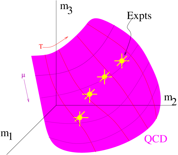
Figure 1: As $T$ and $\mu$ are varied, the QCD predictions lie on a surface in the space of measurements $(m_{1},m_{2},m_{3})$. The data will lie on this surface if all non-thermal behaviour has been properly removed. In the happiest case, this could yield a comparison with QCD and a measurement of $T$ and $\mu$. Deviations from the surface only in a small window of beam energy is a signal for the CEP.

In order to remove unmeasurable quantities like $V$ and $T$ from explicitly appearing in the measurements one has to construct different combinations of variables. Once all backgrounds and systematics are under control, the following combinations can be compared to QCD predictions—

$$m_{1} = {\cal S}\sigma=\frac{\left[B^{3}\right]}{\left[B^{2}\right]}=\frac{\chi^{(3)}/T}{\chi^{(2)}/T^{2}}=\frac{1}{r_{23}},$$

$$m_{2} = {\cal K}\sigma^{2}=\frac{\left[B^{4}\right]}{\left[B^{2}\right]}=\frac{\chi^{(4)}}{\chi^{(2)}/T^{2}}=\frac{2}{r_{24}^{2}},$$

$$m_{3} = \frac{\cal K}{\cal S}\sigma=\frac{\left[B^{4}\right]}{\left[B^{3}\right]}=\frac{\chi^{(4)}}{\chi^{(3)}/T}=\frac{2}{r_{34}}.$$ (6)

These three measurements can be used to extract $\chi^{(2,3,4)}$ under the assumption that all backgrounds have been removed and a comparison with lattice QCD predictions [3] is possible. However this is a strong assumption.

A neater analysis with less bias is possible. Plot the experimentally measured values of $(m_{1},m_{2},m_{3})$ in a three-dimensional plot. Lattice QCD predictions of these quantities can also be plotted in the same figure (see Figure 1). As one varies $T$ and $\mu_{B}$, the theoretical predictions trace out a surface. If the experimental points do not lie on it, then non-thermal sources have not been completely removed. On the other hand, if they do, then one can estimate the values of $T$ and $\mu_{B}$ the experiments correspond to by comparison with the QCD predictions.

Near a critical point, one can never satisfy $V/\xi^{3}\gg 1$. As a result the central limit theorem will break down. In a static system one would expect the Kurtosis to diverge. However the expansion of the fireball rounds off the transition and renders $\xi$ finite [13]. Nevertheless, $\xi$ has a maximum near the CEP. Since ${\cal K}\simeq\xi^{3}$ [14] the Kurtosis peaks near the CEP. For the measurements suggested above, one would have

$$m_{1}\propto\xi^{(7-\eta)/2},\qquad m_{2}\propto\xi^{5-\eta},\qquad m_{3}\propto\xi^{(5-\eta)/2}.$$ (7)

In other words, all these quantities would have non-monotonic behaviour as a function of the beam energy if the beam-energy scan passes through the vicinity of the CEP. If desired, such analyses can be easily extended to higher cumulants (when the system deviates from a Gaussian, the higher cumulants become easier to measure).

One can use the plot of Figure 1 in the search for the CEP. Tune the background subtraction and cuts so that the present data for $(m_{1},m_{2},m_{3})$ lie on the QCD surface, as it should. Then in a beam energy scan, the data will lie on the surface whenever the system lies away from the CEP. In the vicinity of the CEP, however, effects such as those discussed in [13] drive the system away from thermodynamic equilibrium. As a result, in this small window of energies the experimental data will deviate from the surface, signaling critical slowing down as a direct probe of the nearness of the CEP.

References

- [1] R. V. Gavai and S. Gupta, Phys. Rev., D 68 (2003) 034506.
- [2] R. V. Gavai and S. Gupta, Phys. Rev., D 71 (2005) 114014.
- [3] R. V. Gavai and S. Gupta, Phys. Rev., D 78 (2008) 114503.
- [4] M. Cheng, et al., Phys. Rev., D 79 (2009) 074505.
- [5] P. de Forcrand and O. Philipsen, J. H. E. P., 0701 (2007) 077.
- [6] O. Philipsen, these proceedings.
- [7] R. V. Gavai and S. Gupta, Phys. Rev., D 73 (2006) 014004.
- [8] R. V. Gavai, S. Gupta and R. Ray, Prog. Theor. Phys. Suppl., 153 (2004) 270.
- [9] M. A. Stephanov, K. Rajagopal, E. V. Shuryak, Phys. Rev., D 60 (1999) 114028.
-
[10]
M. Asakawa, U. W. Heinz and B. Muller, Phys. Rev. Lett., 85 (2000) 2072;
S. Jeon and V. Koch, Phys. Rev. Lett., 85 (2000) 2076. - [11] B. Mohanty (STAR Collaboration), arXiv:0907.4476 [nucl-ex].
-
[12]
D. T. Son and M. A. Stephanov, Phys. Rev., D 70 (2004) 0506001;
S. Gavin and M. Abdel-Aziz, Phys. Rev., C 70 (2004) 034905;
R. B. Bhalerao and S. Gupta, Phys. Rev.C 79 (2009) 064901. - [13] B. Berdnikov and K. Rajagopal, Phys. Rev., D 61 (2000) 105017.
- [14] M. A. Stephanov, Phys. Rev. Lett., 102 (2009) 032301.