Finite size effects in global quantum quenches: examples from free bosons in an harmonic trap and the one-dimensional Bose-Hubbard model

Abstract

We investigate finite size effects in quantum quenches on the basis of simple energetic arguments. Distinguishing between the low-energy part of the excitation spectrum, below a microscopic energy-scale, and the high-energy regime enables one to define a crossover number of particles that is shown to diverge in the small quench limit. Another crossover number is proposed based on the fidelity between the initial and final ground-states. Both criteria can be computed using ground-state techniques that work for larger system sizes than full spectrum diagonalization. As examples, two models are studied: one with free bosons in an harmonic trap which frequency is quenched, and the one-dimensional Bose-Hubbard model, that is known to be non-integrable and for which recent studies have uncovered remarkable non-equilibrium behaviors. The diagonal weights of the time-averaged density-matrix are computed and observables obtained from this diagonal ensemble are compared with the ones from statistical ensembles. It is argued that the “thermalized” regime of the Bose-Hubbard model, previously observed in the small quench regime, experiences strong finite size effects that render difficult a thorough comparison with statistical ensembles. In addition, we show that the non-thermalized regime, emerging on finite size systems and for large interaction quenches, is not related to the existence of an equilibrium quantum critical point but to the high energy structure of the energy spectrum in the atomic limit. Its features are reminiscent of the quench from the non-interacting limit to the atomic limit.

The study of the non-equilibrium evolution of closed quantum many-body systems has been triggered by the recent progresses in cold atoms experiments in which atoms are hardly coupled to the environment Greiner2002 ; Experiments . Furthermore, microscopic parameters of the Hamiltonian governing the dynamics can be controlled at will and changed on microscopic timescales. In this context, the question of the unitary evolution of an isolated quantum system after a sudden change of one parameter, the so-called quantum quench, has attracted a lot of interest in both the experimental and theoretical communities Moeckel2009 . Many different questions are raised by such a set-up, among which are the relaxation of observables Igloi2000 ; Sengupta2004 ; Rigol2006 ; Cazalilla2006 ; Perfetto2006 ; Calabrese2006 ; Calabrese2007 ; Kollath2007 ; Manmana2007 ; Gangardt2008 ; Hackl2008 ; Babadi2009 ; Hackl2009 ; Barthel2009 , the question of thermalization Peres1984 ; EarlyETH ; Deutsch1991 ; Srednicki1994 ; Srednicki1994a ; Srednicki1999 ; Skrovseth2006 ; Rigol2007 ; Kollath2007 ; Brody2007 ; Rigol2008 ; Reimann2008 ; Moeckel2008 ; Rossini2009 ; Eckstein2009 ; Rigol2009 ; Rigol2009a ; Sotiriadis2009 , the existence of a subsystem steady-state Barthel2008 ; Cramer2008 ; Cramer2008a ; Flesch2008 , and the propagation of the entanglement Calabrese2005 ; Chiara2006 ; Lauchli2008 ; Fagotti2008 ; Manmana2009 . Beyond these academic concerns, practical applications of quenches have been proposed through the engineering of metastable states Heidrich-Meisner2008 ; Heidrich-Meisner2009 and of an out-of-equilibrium supersolid state in a cold atoms set-up Keilmann2009 . This paper is dedicated to the thermalization issue, but restricted to specific examples and without claims on general results about the thermalization mechanism. In this context, a quench can be understood as a way to create an initial state that evolves through the dynamics of a given Hamiltonian. A common wisdom in classical mechanics is that the long-time evolution will forget about the initial state and will explore all the accessible phase-space, provided the dynamics are chaotic. Then, ergodicity allows for the use of statistical ensembles in place of time-averaging. For a closed quantum system, as the evolution is unitary and the spectrum discrete, long-time recurrences occur and the contribution of the eigenstates involved in the dynamics is fixed by the initial state. For large enough systems, a quantum ergodic theorem was proposed Neumann1929 , supporting the emergence of the microcanonical ensemble which is the usual statistical ensemble for an isolated system. This approach aims at showing that time-averaged density-matrix $\bar{\rho}$ (see below for the definition) is macroscopically equivalent to the microcanonical ensemble. In a quantum quench, the initial state is not a “typical” state of a given energy but usually is the ground-state of the same Hamiltonian with different parameters. Consequently, the quench amplitude, or how much do we change the Hamiltonian, is here another relevant quantity. Another way to regard a quench can be as a perturbation of the initial state and one may wonder whether the long-time response is sensitive to the initial state. Furthermore, numerical tools and experiments on closed systems cannot easily reach a large number of particles so finite size effects can be important in the interpretation of the observed phenomena. This paper suggests possible approaches to the question of these finite size effects after a quantum quench, and a possible interpretation of the observations made on a particular model: the one-dimensional Bose-Hubbard model. The other model, consisting of free bosons in an harmonic trap, offers another example of finite size effects and remarkable behaviors. Some of the features of the two models are surprisingly connected.

The central object governing the long-time physics after a quantum quench is the time-averaged density-matrix $\bar{\rho}$ that predicts the time-averaged expectation values of any observable. This density-matrix has also connections to the heat or work done on a system Silva2008 ; Dorosz2008 ; Barankov2008 ; Polkovnikov2008c . The weights of this “diagonal ensemble” are difficult to compute for large systems as one needs to fully diagonalize the Hamiltonian so one unfortunately has to work with small systems (Hilbert spaces). Other methods have been used to tackle the physics of quenches. For instance, “Ab-initio” numerics have been used on both integrable and non-integrable models EarlyETH ; Kollath2007 ; Manmana2007 ; Rigol2008 ; Eckstein2008 ; Kollar2008 ; Barthel2008 ; Cramer2008a ; Flesch2008 ; Roux2009 ; Biroli2009 . Numerical methods like time-dependent density-matrix renormalization group (tDMRG) Vidal2004 ; White2004 ; Daley2004 can be used to compute the time-evolution of the wave-function but the interpretation is restricted to observables and to a finite window of time, and cannot give access the these weights. Exact results on integrable models Igloi2000 ; Rigol2007 ; Barthel2008 ; Cramer2008a ; Flesch2008 ; Barmettler2009 ; Faribault2009 ; Li2009 ; Biroli2009 have the advantage to treat in a non-perturbative way large systems, but on the other hand, it is not surprising that they do not always thermalize due to the extensive number of conserved quantities. Luttinger liquid theory, which describes the low-energy physics of one-dimensional models in terms of free bosonic fields (thus an integrable theory), has been used to compute the time-evolution of the observables Calabrese2006 ; Cazalilla2006 ; Perfetto2006 ; Iucci2009 ; Uhrig2009 . Quantum chaos methods have also helped studying the time-evolution of the Bose-Hubbard model Bodyfelt2007 ; Cassidy2009 ; Hiller2009 . Some studies focused on the relation between fidelity and on the energy distribution Roux2009 ; Zanardi . All these methods suffer from approximations and/or finite size effects and it is sometimes hard to determine what is an artifact or not.

Some of the results from numerical simulations seems to be contradictory Kollath2007 ; Manmana2007 ; Rigol2008 ; Roux2009 ; Rigol2009 ; Rigol2009a but were carried out on different models with different range of parameters, and not necessarily starting from the ground-state Rigol2008 of a simply related Hamiltonian. Performing a quantum quench amounts to projecting an initial state onto the energy spectrum of the final Hamiltonian, corresponding to a certain distribution of energy $\bar{\rho}(E)$. In the thermodynamical limit, a global quench is expected to drive the mean energy to the bulk of the energy spectrum since the perturbing operator is extensive. In this high energy domain, semi-classical physics and random-matrix theory arguments are expected to work and make expectation values hardly depend on the energy (within a window given by the energy fluctuations) Peres1984 ; Deutsch1991 ; Srednicki1994 : thermalization can occur in the sense that the energy distribution obtained from the quench gives the same averages for the observables as the microcanonical ensemble. This so-called “eigenstates thermalization hypothesis” (ETH) has been tested numerically EarlyETH ; Rigol2008 ; Rigol2009 ; Rigol2009a for given models (typically fermionic and hard-core bosonic models) and some given set of parameters. No memory of the initial state (for a given mean energy) is thus found on simple observables. These results agree well with the previous findings of Ref. Manmana2007, on a similar model. Having in mind this qualitative argument, the results of Ref. Kollath2007, on the non-integrable one-dimensional (1D) Bose-Hubbard model (BHM) look rather counter-intuitive: for small quenches, a thermalized regime was found in the sense that two independent observables computed within a (grand)-canonical ensemble (and not microcanonical) and from time-evolution gave the same results. On the contrary, a mean-field treatment of the 1D BHM interpreted in the framework of chaos theory Cassidy2009 supports non-thermalization below an interaction threshold and thermalization above (mean-field theory is however known to fail for this strongly-correlated model so the results are not under control). The findings of Ref. Kollath2007, were later supported by the calculation of the diagonal ensemble distributions which looked like an approximate Boltzmann law Roux2009 in the small quench regime. Surprisingly, for large quenches, a non-thermalized regime was found in Ref. Kollath2007, in which the correlations bear a strong memory of the initial state (in the sense that they are closer to the ones in the initial state than to the thermalized ones). This non-equilibrium behavior was attributed to the very peculiar shape of the diagonal ensemble in this regime Roux2009 . An important step towards the understanding of the non-thermalized regime on finite size systems was made very recently Biroli2009 by giving numerical evidences on the 1D BHM that ETH does not apply for large quenches in finite systems and suggesting a general framework in terms of rare events contributing to the distribution, providing a refined version of the ETH.

As integrability is often one of the ingredients that play a role in the physics of quenches, we briefly recall that, for 1D quantum many-body models, integrability can be well defined for a class of models which have the property of scattering without diffraction Sutherland2004 . This has two consequences that are in relation with the question of thermalization: the momenta of the particles do not redistribute Sutherland2004 (a process which is believed to be essential to get the thermalized momentum distribution), and there is an extensive number of conserved quantities that separate the eigenstates in many sectors, constraining the time evolution. In the context of nuclear physics, random-matrix theory has been proposed to describe the statistical features of the bulk of the spectrum and it is commonly conjectured that non-integrable quantum many-body or classically chaotic models display universal level statistics RMT . Level statistics have been computed in a few many-body models RMT-Many-body , supporting the conjecture, but these results are restricted to a few models and it cannot be excluded that diffractive models could display non-universal level statistics. The Bose-Hubbard model is a bit peculiar in this sense: if one denotes by $N_{\textrm{max}}$ the maximum number of bosons onsite, the model is non-diffractive only for $N_{\textrm{max}}=1$ Kollath2010 . In addition, if $U$ is the interaction strength, $U=0$ is an integrable point (the atomic limit $J=0$ is as well exactly solvable). Level statistics and delocalization properties of the eigenstates have shown Kollath2010 ; Kolovsky2004 that the BHM display features of quantum chaotic systems for non-zero $U$ (and larger $N_{\textrm{max}}$).

The first goal of this paper is to discuss the crossover from small to large quench amplitude regimes on the basis of energetic and static fidelity arguments, and to evaluate the finite size effects that are associated to this crossover. We then turn to a detailed discussion of the diagonal ensemble and the verification of the ETH in the BHM, complementary to what has been done in Refs. Roux2009, and Biroli2009, . We show that the observed Boltzmann-like regime is spoiled by strong finite size effects that prevent both an accurate definition of an effective temperature and the comparison with the microcanonical ensemble. In the large quench limit, we explain in details that the breakdown of the ETH is actually related to the “integrable” quench limit $U_{i}=0\rightarrow U_{f}=\infty$. Thus, non-thermalization in the 1D BHM is, on finite systems, reminiscent of the atomic limit. While the $U=0$ limit of the Bose-Hubbard model is trivially integrable as a free boson model, the infinite $U$ (or atomic) limit is a bit particular: for very large $U$ and focusing on the low-energy part of the spectrum, the model is effectively identical to an integrable 1D hard-core bosons model ($N_{\textrm{max}}=1$). However, we will see that, to understand the large-$U$ limit of the quench, we will have to consider the whole excitation spectrum and not only the low-energy part. This result can be qualitatively and partially connected to the effect of the proximity to integrable points in quantum quenches, studied very recently in fermionic and hard-core bosonic models Rigol2009 ; Rigol2009a , in the sense that the observed non-thermalized regime on finite systems is connected to a particular limit in which the model has high degeneracies. Throughout the paper, we also give a simple but interesting example of a quench in a toy model consisting of free bosons confined in an harmonic trap. The motivation for it is that it surprisingly shares some qualitative features with the 1D BHM and that it allows for analytical calculations on some properties of the diagonal ensemble distribution. This model also corresponds to a standard experimental setup (so for the BHM) although interactions would have to be taken into account for a realistic comparison.

The paper is organized as follows: we first review in Sec. I the definitions of the time-averaged density-matrix, the ETH and the computation of the diagonal weights for the two models under study. In Sec. II, we suggest two kinds of crossover number of particles to distinguish the small and large quench regimes. Lastly, we discuss in Sec. III the fate of the ETH in the 1D BHM and on small finite size systems.

I Models and computation of the weights of the diagonal ensemble

I.1 The time-averaged density-matrix and the “eigenstate thermalization hypothesis”

As discussed in recent papers Rigol2008 ; Roux2009 ; Faribault2009 ; Rigol2009 ; Rigol2009a ; Biroli2009 , the time-averaged expectation values of any observable are governed by the time-averaged density-matrix $\bar{\rho}$, which is diagonal in the final Hamiltonian eigenstate basis, provided the spectrum is non-degenerate. From now on, we only consider finite size systems that have a discrete spectrum. This leads to the so-called “diagonal ensemble” that has weights fully determined by the overlaps between the initial state $\left|{\psi_{0,i}}\right\rangle$ and eigenstates $\left|{\psi_{n,f}}\right\rangle$ of the final Hamiltonian $\mathcal{H}_{f}$. Usually, $\left|{\psi_{0,i}}\right\rangle$ is the ground-state of the initial Hamiltonian $\mathcal{H}_{i}$ and we assume in the following that we start from this zero-temperature pure state. We also consider that the final Hamiltonian takes the form

$$\mathcal{H}_{f}=\mathcal{H}_{i}+\lambda\mathcal{H}_{1}\;,$$ (1)

where $\lambda$ (that has the dimension of an energy) is called the quench amplitude, and $\mathcal{H}_{1}$ is the dimensionless perturbing operator. Working on a global quantum quench means that $\mathcal{H}_{1}$ is assumed to be an extensive operator that scales with the number of particles $N$. The time-averaged density-matrix is defined by $\bar{\rho}=\lim_{t\rightarrow\infty}\frac{1}{t}\int_{0}^{t}\left|{\psi(s)}\right\rangle\left\langle{\psi(s)}\right|ds$ with $\left|{\psi(t)}\right\rangle=e^{-i\mathcal{H}_{f}t}\left|{\psi_{0,i}}\right\rangle$. It is important to realize that the infinite time limit is taken before the thermodynamical limit. If the spectrum has exact degeneracies, the time-averaged density-matrix reads:

$$\bar{\rho}=\sum_{n}p_{n}\left|{\psi_{n,f}}\right\rangle\left\langle{\psi_{n,f}}\right|+\sum_{d}\left|{\psi_{d,f}}\right\rangle\left\langle{\psi_{d,f}}\right|$$ (2)

where $n$ labels non-degenerate eigenstates of $\mathcal{H}_{f}$ and $p_{n}=|{\langle{\psi_{n,f}}|{\psi_{0,i}}\rangle}|^{2}$ are the diagonal weights. $d$ labels the basis of the degenerate subspaces, and the vectors $\left|{\psi_{d,f}}\right\rangle=\sum_{q_{d,f}}\langle{q_{d,f}}|{\psi_{0,i}}\rangle\left|{q_{d,f}}\right\rangle$ keep a memory of the initial phases of $\left|{\psi_{0,i}}\right\rangle$ with respect to the $\left|{q_{d,f}}\right\rangle$. In the situation where $\bar{\rho}$ is block-diagonal, in order to get time-averaged results for an observable $\mathcal{O}$ which has off-diagonal matrix elements in the $\mathcal{H}_{f}$ eigenstate basis, one would have to compute all the overlaps $\langle{q_{d,f}}|{\psi_{0,i}}\rangle$ and $\langle{q^{\prime}_{d,f}}|{\mathcal{O}}|{q_{d,f}}\rangle$ and sum up the contributions of all a degenerate subspace. In the following, this would be the case only for the free boson model and we will actually only use observables that are diagonal because the dimensions of the degenerate sectors grows (roughly) exponentially with the number of bosons $N$. For the Bose-Hubbard model, one can check that the spectra are non-degenerate in each symmetry sector.

For a generic non-integrable model, the “eigenstate thermalization hypothesis” (ETH) has been surmised Deutsch1991 ; Srednicki1994 ; Srednicki1994a ; Srednicki1999 ; Rigol2008 , suggesting an explanation for thermalization in an isolated quantum system and a justification for the use of the microcanonical ensemble. The ETH is supported by semi-classical and random-matrix theory arguments Peres1984 ; Deutsch1991 ; Srednicki1994 ; Srednicki1994a ; Srednicki1999 , and was checked numerically on particular models EarlyETH ; Rigol2008 ; Rigol2009 ; Rigol2009a . The ETH boils down to the fact that, in a given small window of energy, the diagonal observables $\mathcal{O}_{n}=\langle{\psi_{n,f}}|{\mathcal{O}}|{\psi_{n,f}}\rangle$ that contribute to the time-averaged expectation value $\bar{\mathcal{O}}=\textrm{Tr}[\bar{\rho}\mathcal{O}]=\sum_{n}p_{n}\mathcal{O}_{n}$ hardly depend on the eigenstate $n$ (in short, $\mathcal{O}_{n}\simeq\bar{\mathcal{O}}$ in a small energy window). Consequently, any distribution peaked around the mean energy, and one can show on general grounds that the relative width of the distribution scales to zero as $N^{-1/2}$ Rigol2008 (although some slower scalings could occur Roux2009 ), will give the same observables as the microcanonical ensemble, therefore accounting for thermalization. For integrable models Rigol2008 ; Rigol2009 ; Rigol2009a , non-thermalization is explained from the fact that observables fluctuate a lot within a given energy window, which may be associated with the extensive number of conserved quantities that exist in these models. A more subtle scenario for the breakdown of the ETH was recently proposed Biroli2009 , in which some “rare” states have a significant contribution to the averaged observables.

I.2 Free bosons in an harmonic trap

We now describe how to get the diagonal weights for two particular models. Firstly, we consider a model of $N$ non-interacting bosons initially confined in an harmonic trap of frequency $\omega_{i}$ and lying in the zero-temperature ground-state. The frequency is changed to $\omega_{f}$ at time $t=0$. For this model, the quench amplitude is defined as $\lambda=\omega_{f}/\omega_{i}-1$ (taking $\omega_{i}$ as the unit of energy), according to the expression of the quench parameter in terms of the harmonic oscillator ladder operators. We start with the computation of the single-particle wave-function overlaps $\mathfrak{p}_{n}$ since the results for the many-body wave-function will be expressed as a function of them. The single-particle spectrum is non-degenerate and the single-particle eigenfunctions are:

$$\phi_{n}(x)=\frac{1}{\sqrt{2^{n}n!\sqrt{\pi}\sigma}}e^{-\frac{x^{2}}{2\sigma^{2}}}H_{n}\left(\frac{x}{\sigma}\right)\;,$$

with $\sigma=\sqrt{\hbar/m\omega}$ and $H_{n}$ the Hermite polynomials. The single-particle excitation spectrum is split into the odd and even parity sectors and the overlaps are non-zero for even-parity wave-functions only. They read:

$$\mathfrak{p}_{2n}=\frac{(2n)!}{2^{2n}(n!)^{2}}\frac{\sqrt{1+\lambda}}{1+\lambda/2}\left(\frac{\lambda}{\lambda+2}\right)^{2n}$$ (3)

for integer $n$. The many-body wave-function of an $N$-bosons excited configuration $\{n_{j}\}=\{n_{0},\cdots,n_{m}\}$ of the final Hamiltonian $\mathcal{H}_{f}$ (with highest occupied level $m$) is:

$$\left|{\{n_{j}\}}\right\rangle=\sqrt{\frac{n_{0}!n_{1}!\cdots n_{m}!}{N!}}\sum_{p\in\mathcal{P}}\left|{\phi_{1,f}{:}{p(1)},\cdots,\phi_{m,f}{:}{p(N)}}\right\rangle\;.$$

with $\mathcal{P}$ the set of all permutations and $n_{j}$ the occupation of the single-particle orbital $\phi_{j,f}$. Overlapping this state with the $N$-bosons initial ground-state $\left|{\phi_{0,i},\cdots,\phi_{0,i}}\right\rangle$ gives the many-body weights

$$p_{\{n_{j}\}}=N!\frac{(\mathfrak{p}_{0})^{n_{0}}}{n_{0}!}\frac{(\mathfrak{p}_{2})^{n_{2}}}{n_{2}!}\cdots\frac{(\mathfrak{p}_{m})^{n_{m}}}{n_{m}!}$$ (4)

In this equation, all $m$’s are even integers. The total energy of this excitation is $E_{\{n_{j}\}}=\hbar\omega_{f}(2n_{2}+4n_{4}+\cdots+mn_{m})+\hbar\omega_{f}N/2$ with the constraint $\sum_{j=0}^{m/2}n_{2j}=N$. Eq. (4) is nothing but the multinomial distribution associated with the elementary probabilities $\mathfrak{p}_{m}$ and it is thus clear that it is normalized. We also see that formula (4) is in general valid for a free boson model, starting from the condensed ground-state (and specifying the $\mathfrak{p}_{m}$). If one takes the single-particle Boltzmann factor for the $\mathfrak{p}_{m}$, one recovers the many-body Boltzmann factor for the configuration. Contrary to statistical ensemble distributions, the weights do not show a simple dependence of the configuration energy. This quench is qualitatively similar to a Joule compression/expansion as the 1D effective density $n=N\omega$ suddenly changes. In fact, $\lambda=n_{f}/n_{i}-1$ is related the ratio of the effective densities. Other examples of quantum mechanical treatments of the Joule expansion can be found in the literature Camalet2008 ; Aslangul2008 .

In order to get the distribution of the weights versus energy, we resort to numerics: using a fixed number of low-lying even parity levels $N_{s}$, we scan all possible configurations of $N$ bosons in these $N_{s}$ levels iteratively up to roughly $62\times 10^{9}$ configurations ($N=18$ and $N_{s}=22$). The truncation error associated with a finite $N_{s}$ is checked by summing up the weights.

I.3 The one-dimensional Bose-Hubbard model

The Bose-Hubbard model in a one-dimensional lattice, known to be non-integrable for $U\neq 0$, is described by the following Hamiltonian:

$$\mathcal{H}=-J\sum_{j}[b^{{\dagger}}_{j+1}b_{j}+b^{{\dagger}}_{j}b_{j+1}]+\frac{U}{2}\sum_{j}n_{j}(n_{j}-1)\,,$$

with $b^{{\dagger}}_{j}$ the operator creating a boson at site $j$ and $n_{j}=b^{{\dagger}}_{j}b_{j}$ the local density. $J$ is the kinetic energy scale while $U$ is the magnitude of the onsite repulsion. In an optical lattice, the ratio $U/J$ can be tuned by changing the depth of the lattice and using Feshbach resonance. When the density of bosons is fixed at $n=1$ and $U$ is increased, the zero-temperature equilibrium phase diagram of the model displays a quantum phase transition from a superfluid phase to a Mott insulating phase in which particles are localized on each site. The critical point has been located at $U_{c}\simeq 3.3J$ using numerics Kuhner2000 . The quenches are performed by changing the interaction parameter $U_{i}\rightarrow U_{f}$ (we set $J=1$ as the unit of energy in the following), so we have $\lambda=(U_{f}-U_{i})/2$, and the perturbing operator $\mathcal{H}_{1}=\sum_{j}n_{j}(n_{j}-1)$ is diagonal. Numerically, one must fix a maximum onsite occupancy $N_{\textrm{max}}$ and we take $N_{\textrm{max}}=4$ unless stated otherwise. Exact diagonalization calculations are carried out using periodic boundary conditions and translational invariance. We denote by $0\leq k\leq L-1$ the total momentum symmetry sectors. The algorithm to get the ground-state and eigenstates of the Hamiltonian is a full diagonalization scheme for sizes up to $L=10$ at unitary filling. For some of the quantities, we use the Lanczos algorithm up to $L=15$. In Ref. Roux2009, , the Lanczos algorithm has been proposed to compute the low-energy weights of the distribution. This worked relatively well for the 1D BHM, and in particular for the spectrum-integrated quantities but it may not be suited for all possible kind of quenches. We notice that in the case of quenches with a mean energy deep in the bulk of the spectrum, a generalization of the Lanczos algorithm Ericsson1980 that works in the bulk of a spectrum could be used to get the main weights. For what we call small quenches in the following, the larger weights are in the low-energy region so Lanczos can generically give good results in such situations.

II Arguments on finite size effects and the different regimes of a quantum quench

The goal of this part is to quantify the distance of the quench distribution $\bar{\rho}(E)$ from the many-body ground-state and the low-energy region of the spectrum. A first distance is defined from an energetic argument and a second one from the overlap with the ground-state of $\mathcal{H}_{f}$. Both criteria leads to a crossover number of bosons $N_{c}(\lambda)$ that can be computed numerically and that diverge with small $\lambda$ as a power-law. When $N\ll N_{c}$, the quench probes the low-energy part of the spectrum while when $N\gg N_{c}$, high-energy physics govern the time-evolution. Both definitions do not depend on the integrability of the model but we may argue that for non-integrable models, there is a strong qualitative difference between the low-energy part of the spectrum and the bulk of the spectrum. These finite-size effects are rather generic while other kind of finite-size effects can emerge for a given model: this will be for instance the case for the BHM at large $U$.

II.1 Crossover number of particles from an energetic argument

Figure 1: A typical many-body spectrum of a finite-size system: this example is taken from the 1D Bose-Hubbard model with $U_{f}/J=2.5$ and $L=N=10$. Energies are given as a function of the total momentum $k$. The width of the spectrum is typically proportional to $N$ or $N^{2}$ depending on the statistics. Zooms in the low-energy region and in the bulk of the spectrum (grey region) are given. The low-energy region features elementary excitations up to a typical energy scale $\Delta_{f}$ which is assumed to be microscopic, i.e. non-extensive. Here, we take $\Delta_{f}=U_{f}$ and the relation dispersion of the excitation branch is sketch (the line is a guide to the eyes).

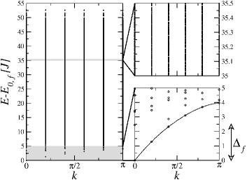
The low-energy part of the spectrum – We first have to specify what we mean by the low-energy region of the spectrum: it corresponds to the typical energies of a few elementary excitations above the ground-state. These elementary excitations are quasi-particles, collectives modes, particle-hole excitations…Single or few excitations give a structure (dispersion relations, continuum of low-lying excitations) to the low-energy part of the many-body spectrum (see an example in Fig. 1). We denote by $\Delta_{f}$ the typical energy scale of a single excitation, it is a microscopic energy scale. In Bethe-ansatz solvable or free systems, a high energy excitation can be understood as a superposition of single-particle excitations while this is no longer true for non-integrable systems RMT ; RMT-Many-body . If the number of elementary excitations remains small enough, they may hardly interact and have integrable-like features in the low-energy part of the spectrum. We thus expect a smooth crossover between integrable-like and non-integrable like behaviors with increasing the energy above the ground-state, but the typical energy of this crossover is hard to evaluate, except that it must be above $E_{0,f}+\Delta_{f}$.

Figure 2: (Color online) Sketch of the energy scales in a quantum quench. The initial state builds up an energy distribution $\bar{\rho}(E)$ (diagonal ensemble) around a mean energy $\bar{E}$ fixed by the initial state. The quench amplitude $\lambda$ tunes both $\bar{E}$ and the ground-state energy $E_{0,f}$ and the low-energy scale $E_{f}^{*}$. $\Delta_{f}=E_{f}^{*}-E_{0,f}$ is assumed to be non-extensive while $E_{0,f}$ and $\bar{E}$ are extensive. $\bar{E}=E_{f}^{*}$ defines the crossover number of particles $N_{c}$. In the thermodynamical limit, one expects $\bar{E}\gg E_{f}^{*}$ for any finite $\lambda$.

Criteria – We consider that the energy distribution $\bar{\rho}(E)$ is centered around the the mean energy $\bar{E}=\langle{\psi_{0,i}}|{\mathcal{H}_{f}}|{\psi_{0,i}}\rangle$ of the distribution (fixed by the initial state) as in general $\Delta E/(\bar{E}-E_{0,f})\sim 1/\sqrt{N}$. Since $\left|{\psi_{0,i}}\right\rangle$ is not an eigenstate of $\mathcal{H}_{f}$, we necessarily have $\bar{E}>E_{0,f}$. The criteria we choose to distinguish between low-energy (or small) quenches and high-energy (or large) quenches is $\bar{E}=E^{*}_{f}$ (see Fig. 2) where $E_{f}^{*}$ is such that $E_{f}^{*}-E_{0,f}=\Delta_{f}$ with the ground-state energy $E_{0,f}$. It corresponds to the situation where the mean-energy put into the system excites roughly only one elementary excitation and is thus a finite-size effect. Another way to introduce the same criteria is the following: $(\bar{E}-E_{0,f})/\Delta_{f}$ is the energy difference between the initial state and the final ground-state in units of the typical elementary excitation energy $\Delta_{f}$, the criteria corresponding to a distance of one $\Delta_{f}$ . The criteria thus amounts to a lower bond of the energies at which one enters in the bulk of the spectrum. The order of magnitude of $\Delta_{f}$ is set by the microscopic units of energy of the model. For instance, we’ll take $U_{f}$ in the BHM as it controls the sound velocity in the superfluid region and the Mott gap in the Mott phase.

This criteria gives a relation between the crossover number of particles $N_{c}$ (on a lattice we work at finite density so it also corresponds to a crossover length $L_{c}$) and the quench amplitude $\lambda$ is such that, if $N\ll N_{c}(\lambda)$, the energy is mostly distributed among the low-energy excitations while if $N\gg N_{c}(\lambda)$, most of the weights are on high-energy excitations. We can rewrite the criteria in a more tractable way: using the notation $e=E/N$ for the energy per particle, and the label $0$ for ground-state energies, it reads

$$N_{c}(\lambda)=\frac{\Delta_{f}(\lambda)}{\bar{e}(\lambda)-e_{0,f}(\lambda)}\;.$$ (5)

Interestingly, we expect $N_{c}(\lambda)$ to generically diverge as $\lambda^{-2}$ in the limit of small $\lambda$. Indeed, we have $\bar{e}=e_{0,i}+\lambda h_{1,i}$ with $h_{1,i}=\langle{\psi_{0,i}}|{\mathcal{H}_{1}}|{\psi_{0,i}}\rangle/N$, the expansion $e_{0,f}\simeq e_{0,i}+(de_{0}/d\lambda)_{i}\lambda+(d^{2}e_{0}/d\lambda^{2})_{i}\lambda^{2}/2$, and $(de_{0}/d\lambda)_{i}=h_{1}$ after Feynman-Hellman theorem. With Eq. (1), one finally gets $N_{c}(\lambda)\lambda^{2}\rightarrow 2\Delta_{i}/(d^{2}e_{0}/d\lambda^{2})_{i}$ at $\lambda\rightarrow 0$.

A few comments can be made on the criteria:

• When comparing quenches from the same initial state but with different $\mathcal{H}_{f}$, $\lambda$ controls the mean energy per particle put into the system. Thus, $\lambda$ is a meaningful parameter even in the thermodynamical limit.

• This definition looks qualitative due to the rather arbitrary choice of $\Delta_{f}$ and to the fact that, on finite systems, the energy distribution can have a rather large width associated with energy fluctuations $\Delta E$. We point out that $N_{c}$ is a crossover number so that $N\simeq N_{c}$ has no particular meaning. Furthermore, from the divergence at small $\lambda$, one can have $1\ll N\ll N_{c}$, i.e. a situation where energy fluctuations vanish.

• When $\lambda$ is scanned from $0$ to a finite value, both the mean energy and the region of the spectrum that plays a role in the time-evolution (around $\bar{e}$) are continuously changed. One can also notice that a quench that starts from a ground-state does not necessarily allow to access any energy of the $\mathcal{H}_{f}$ spectrum, contrary to the situation where one prepares the initial state at will.

• The regimes $N\gg N_{c}$ and $N\ll N_{c}$ are expected to be physically different for generic (non-integrable) systems. Below $\Delta_{f}$, the density of states is usually much smaller than in the bulk of the spectrum: level spacings are of order of $1/N$ and observables can strongly fluctuate with the eigenstate number as it can be seen in Figs. 5 and 6 (similar observations can be made in the figures of Refs. Rigol2008, ; Rigol2009, ; Rigol2009a, ). In this low-energy region, RMT arguments are not expected to work RMT and the eigenstates may not be “typical” so we expect the ETH to fail. These qualitative observations support the difference between the low-energy region and the high-energy region of the spectrum made at the beginning of this section.

  As the full spectrum width grows as $N$ or $N^{2}$ (depending on the statistics of the particles) while the number of eigenstates grows exponentially with $N$, the density of states in the bulk of the spectrum is exponentially large. In this “high-energy” regime (with respect to elementary excitations), semi-classical and RMT arguments are believed to work reasonably well for non-integrable models RMT , which was checked on some strongly correlated systems RMT-Many-body . As observed numerically on several examples Rigol2008 ; Rigol2009 ; Rigol2009a , simple observables hardly depend on the eigenstate number in this regime, supporting the ETH.

• In the thermodynamical limit, we always have $N\gg N_{c}$ and the small quench regime is thus expected to vanish. If one wants to check the ETH on a finite size systems, one needs sufficiently large $\lambda$ in order to try to reach the bulk of the spectrum. However, we will see in this paper a counter-example (the BHM) where ETH fails at large $\lambda$ (see also Ref. Biroli2009, ). Even though it looks difficult to use quenches to probe very low-energy excitations in a very large system, on a finite system, one could tune the mean energy from the low to high energy part of the spectrum using $\lambda$. Furthermore, this small quench regime is certainly of interest for numerical simulations, and also for experiments using a relatively small number of atoms (few hundreds or thousands).

• Lastly, it could be interesting to compare this criteria with the domain of validity of bosonization Cazalilla2006 ; Iucci2009 and conformal field theory Calabrese2006 ; Calabrese2007 but this is beyond the scope of this paper. We note that conformal field theory can describe accurately quenches in certain integrable models in the thermodynamical limit and for arbitrary quench amplitudes Calabrese2006 ; Calabrese2007 . Non-integrable models low-energy features that are described in terms of a free particles (integrable) theory, as bosonization, should display non-thermalized features as for integrable models. In this respect, Ref. Barmettler2009, gives interesting examples on the applicability of these methods to the quench situation.

We now give examples of $N_{c}(\lambda)$ for the two models under study. In the free boson model, the mean energy after the quench can be computed analytically:

$$\bar{e}=e_{0,i}+\frac{\hbar\omega_{f}}{4}\left(\frac{\omega_{f}}{\omega_{i}}-\frac{\omega_{i}}{\omega_{f}}\right)\;,$$

with $e_{0,i/f}=\hbar\omega_{i/f}/2$. The energy fluctuations are given by $\Delta e=(\bar{e}-e_{0,i})\sqrt{2/N}$, showing that the distribution gets peaked in the thermodynamical limit with the usual scaling. A natural choice for $\Delta_{f}$ is $\hbar\omega_{f}$ (the only microscopic energy scale) and the crossover number of bosons can be expressed as a function of the quench amplitude:

$$N_{c}=\frac{\hbar\omega_{f}}{\bar{e}-e_{0,f}}=4\left(\frac{\omega_{i}}{\omega_{f}}+\frac{\omega_{f}}{\omega_{i}}-2\right)^{-1}=4\frac{\lambda+1}{\lambda^{2}}\;.$$

This expression diverges as $4/\lambda^{2}$ in the small quench regime and vanishes as $4/\lambda$ in the large quench regime.

Figure 3: (Color online) Crossover number of bosons $N_{c}$ obtained from the energetic argument in the 1D BHM at filling $n=1$ and starting from $U_{i}=2$. A few points obtained from the criteria based on the static fidelity are also given.

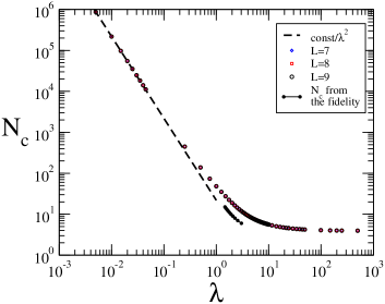
For the 1D BHM, we take $\Delta_{f}=U_{f}$ and $N_{c}$ is given in Fig. 3 for the particular initial value $U_{i}=2$. It displays the expected $\lambda^{-2}$ divergence at small quenches. We notice that the finite size effects on this energy-based criteria are pretty small. This can be put on general grounds for 1D systems: for critical systems the finite-size effects on the ground-state energy per particles have a universal correction Affleck1986 :

$$e_{0}(L)=e_{0}(\infty)-\frac{c\pi u}{6L^{2}}+O\left(\frac{1}{L^{2}}\right)$$

with $u$ the sound velocity and $c$ the central charge. If the system is gapped, the corrections are even smaller as they are exponentially suppressed, by a factor $\exp(-L/\xi)$ with $\xi$ the correlation length enters in the formula. In the large quench limit of the BHM, one can argue that $N_{c}$ saturates to a finite value. Indeed, in the limit of large $\lambda$, one finds that $N_{c}\rightarrow 2/(\langle{n^{2}}\rangle_{0,i}-\langle{n^{2}}\rangle_{0,f})+\mathcal{O}(1/\lambda)\simeq 2/\langle{n^{2}}\rangle_{0,i}$, as the density fluctuations $\langle{n^{2}}\rangle_{0,f}$ are suppressed in the Mott phase. Notice that the energy fluctuations, that scale as $N^{-1/2}$ in the 1D BHM, have been computed numerically in Ref. Roux2009, . The full curve and the two asymptotic behaviors can be simply computed from ground-state calculations.

II.2 Crossover number of particles based on the static fidelity

In the thermodynamical limit, the (squared) fidelity between the two ground-states $\mathcal{F}=|{\langle{\psi_{0,i}}|{\psi_{0,f}}\rangle}|^{2}$ is generally expected to vanish exponentially with the system size or number of particles. Interestingly, $1-\mathcal{F}$ counts the contribution of the excited states to the time-evolution. A possible definition of a crossover number of particles can thus be the value of $\lambda$ and $N$ such that $\mathcal{F}=1/2$, i.e. half of the total weight in the ground-state and half in the excited states. In the limit $\lambda\rightarrow 0$, one can introduce the fidelity susceptibility $\chi_{i,L}$ through the expansion $\mathcal{F}\simeq 1-\lambda^{2}\chi_{i,L}/2$. The scaling of $\chi_{i,L}$ is in general non-trivial. If $\mathcal{H}_{i}$ is gapped, the scaling $\chi_{i,L}\sim L$ has been proposed Venuti2007 , which gives the divergence $N_{c}\sim\lambda^{-2}$. In critical systems, super-extensivity, corresponding to a scaling $\chi_{i,L}/L\sim L^{\alpha_{i}}$ with $\alpha_{i}>0$, can occur Venuti2007 ; Cozzini2007 , leading to a slower divergence $N_{c}\sim\lambda^{-2/(1+\alpha_{i})}$ that depends on the initial state. Notice that we qualitatively expect that the $N_{c}$ from the fidelity will be smaller than the one based on energetic argument because, on sufficiently large systems, $\mathcal{F}$ can be very small while the mean energy is still in the low-energy part of the spectrum.

For the free boson model, the static fidelity as a function of $\lambda$ is $\mathcal{F}=(\sqrt{1+\lambda}/(1+\lambda/2))^{N}$. Setting $\mathcal{F}=1/2$, one has the crossover number of bosons $N_{c}$:

$$N_{c}=\frac{\ln 2}{\ln\left(\frac{1+\lambda/2}{\sqrt{1+\lambda}}\right)}$$ (6)

Notice that it also diverges in the small quench regime as $N_{c}=8\ln 2/\lambda^{2}$ with the same power-law as for the energetic arguments. Put in other words, this means that the many-body ground-state occupation is robust within a $25\%$ change in $\omega$ for $N=10^{2}$, $7\%$ for $N=10^{3}$ and $2\%$ for $N=10^{4}$ (see next section for the single-particle level occupation). In the large amplitude limit, it decreases only logarithmically with $\lambda$, $N_{c}\simeq 2\ln 2/\ln\lambda$ but the prefactor is already small.

The fidelity can also be computed for the 1D BHM by Lanczos calculations. Using the curves $\mathcal{F}(\lambda)$ obtained numerically, we determined $N_{c}(\lambda)$ for numbers of bosons from 6 to 15. The result is plotted in Fig. 3. Due to the relatively small sizes accessible with Lanczos, we cannot investigate the scaling exponent of the small quench divergence. The ground-state fidelity of the 1D BHM has been studied in Ref. Buonsante2007, . We observe that the static fidelity could be computed on larger chains with matrix-product states based algorithms Vidal2004 ; McCulloch2007 or quantum Monte-Carlo techniques Schwandt2009 .

II.3 Quench and transition temperature to the Bose-condensed regime in the free bosons model

The free bosons model undergoes a transition to a Bose-condensed state below a critical temperature $T_{c}$. In the 1D harmonic trap and on a finite size system, the lowest single particle level occupation $\langle{n_{0}}\rangle$ becomes of the order of $N$ below $T_{c}\simeq\hbar\omega N/\ln(N)$ (standard calculations of $T_{c}$ are performed in the grand-canonical ensemble and one sees that for fixed effective density $\omega N$ and $N\rightarrow\infty$, $T_{c}\rightarrow 0$ in agreement with the fact that their is no Bose-condensation in this model in the thermodynamical limit although condensed and non-condensed regimes are clearly seen on finite systems). This critical temperature corresponds to a critical energy $E_{c}-E_{0}\sim\hbar\omega N^{2}$. These standard results can be used to answer the question : whether or not a large quench from the many-body ground-state can drive the system into the non-condensed regime? We found that the mean-energy put into the system scales as $\bar{E}\sim E_{0,f}+\hbar\omega_{f}N\lambda$ so that $\lambda\sim N$ is required to reach $E_{c}$ and the non-condensed regime. This surprising behavior (diverging with the number of bosons) actually agrees with the exact scaling of the single-particle ground-state occupation number which can be computed for the quench since we have seen that the distribution is the multinomial one : we have $\langle{n_{0}}\rangle=Np_{0}\sim N/\sqrt{\lambda}$ at large $\lambda$. Similarly, the fluctuations can be computed and read $\langle{n_{0}^{2}-\langle{n_{0}}\rangle^{2}}\rangle=Np_{0}(1-p_{0})$ so that the relative fluctuations scale as $1/\sqrt{N}$ with a $\lambda$-dependent prefactor. Consequently, starting from the many-body ground-state (for which $\langle{n_{0}}\rangle=N$), one stays in the condensed regime for finite $\lambda$ and one needs $\lambda\sim N^{z}$ with $z>2$ to make $\langle{n_{0}}\rangle$ scale to zero in the thermodynamical limit. The physical origin of the fact that the quench process makes it difficult to reach the critical temperature is that the many-body ground-state has vanishing overlaps with the excited states above $T_{c}$ because they have negligible contributions from the single-particle ground-state. Starting from a finite temperature state, the quench could help cross the critical temperature.

III Diagonal ensemble and thermalization

In this section, we compare averages of the expectation values of observables obtained from different ensembles: the diagonal, microcanonical and canonical ones. We also show the behavior of some local and global observables as a function of the energy per particle to discuss the possibility of thermalization according to the ETH. The first numerical evidences that the ETH does not work for large quenches on finite systems of the 1D BHM were recently given in Ref. Biroli2009, .

III.1 Microcanonical temperature and the density of states

As a preliminary, we discuss the finite size effects and possible issues with the microcanonical ensemble in the model under study. The standard way to define the microcanonical temperature $T_{M}$ of a closed system is from Boltzmann’s formula

$$\frac{1}{T_{M}}=\frac{\partial s_{M}}{\partial\bar{e}}\;,$$ (7)

where we use the entropy per particle $s_{M}=S_{M}/N$ and the statistical entropy $S_{M}(\bar{E})=k_{b}\ln\Omega(\bar{E})$. $\Omega(\bar{E})$ is the number of states within a small energy window $\delta E$ around $\bar{E}$. Any distribution that is peaked enough ($\delta E/\bar{E}\rightarrow 0$ in the thermodynamical limit) will pick up the local density of states $g(\bar{e})$ through $\Omega(\bar{E})\simeq g(\bar{E})\delta E$. Usually, $\delta E$ is taken as the energy fluctuations with $\delta E\sim\bar{E}/\sqrt{N}$. Thus, $\delta E$ is typically much larger than microscopic energy scales such as $\Delta_{f}$. For the free boson model, energies per particle are separated by $\hbar\omega_{f}/N$ and the degeneracy $g(e)$ of each level can be computed numerically for small systems. Asymptotic analytical results exist in the large energy limit for $g(e)$ Abramowitz1965 ; Mekjian1991 ; Comtet2007 . We can thus have access to the microcanonical entropy per particle through $s_{M}=\ln g(e)/N$.

Figure 4: Logarithm of the density of states $g(e)$ as a function of the energy per particle $e$ in the 1D BHM with density $n=1$ for three different interactions. Mott gaps develop at large $U$, splitting the density of states into many lobes separated by $1/N$.

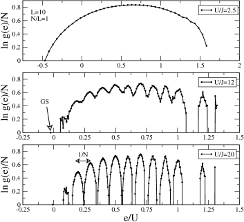
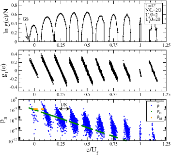
In Fig. 4, we show the logarithm of the density of states of the 1D Bose-Hubbard model on a finite size system ($L=N=10$) for increasing values of the interaction $U$ as a function of the energy per particle in units of $U$. For small interactions, the behavior is smooth and one may safely take the derivative to get the microcanonical temperature. The system has a density of states typical of a bound spectrum Hamiltonian, displaying first positive and then negative temperature regimes. For $U=12J$, in the Mott phase, one observes a gap to the ground-state in the low-energy part of the spectrum and also some oscillations over a typical scale $1/N$. These oscillations are easily understood in the atomic limit ($J=0$) where they correspond to Mott peaks that have a high degeneracy, giving this macroscopic density of states at the center of the lobes. A small $J$ broadens the peaks but the lobes are expected to survive for large enough $U$ in a finite system, as one can see for $U=20J$. In this large-$U$ limit, $e_{0}/U$ gets close to zero while the maximum energy per site is proportional to the number of particles (in Fig. 4, the situation at high energies is a bit different because we cut the maximum number of bosons onsite). The number of Mott lobes being of order $N^{2}$, the density of lobes per unit of $e/U$ grows as $N$ (this remark remains valid with a cut in the maximum number of bosons per site). This means that the density of states, as a function of the energy per site, will be a curve carved into more and more lobes as $N$ increases. For large enough systems, $\delta e$ will be much larger than the inter-lobe distance and will pick up the envelope of the lobes as a local density of states. On finite systems, $\delta e$ and $1/N$ could be of the same order of magnitude, which makes the definition of the microcanonical temperature rather difficult since it is very sensitive to the choice of $\delta e$ and the shape of the peaked distribution.

In the following, the microcanonical ensemble density-matrix $\rho_{M}$ is defined in the usual way:

$$\rho_{M}=\sum_{E_{n}\in[\bar{E}-\delta E,\bar{E}+\delta E]}\frac{1}{\Omega}\left|{\psi_{n,f}}\right\rangle\left\langle{\psi_{n,f}}\right|$$ (8)

with the “free” parameter $\delta E$ as a “small” energy window energy. $\Omega$ is simply the number of eigenstates in the energy window $[\bar{E}-\delta E,\bar{E}+\delta E]$. The sum over the eigenstates of $\mathcal{H}_{f}$ must be taken over all symmetry sectors. Notice that $\delta E$ can be chosen by hand Rigol2008 ; Rigol2009 ; Rigol2009a , or in the same way as the effective canonical temperature will be: by looking for an approximate solution of the equation $\bar{E}=\textrm{Tr}[\rho_{M}\mathcal{H}_{f}]$ (we recall that $\bar{E}=\langle{\psi_{0,i}}|{\mathcal{H}_{f}}|{\psi_{0,i}}\rangle$ is fixed by the initial state). In that case, the solution can be multi-valued so it does not necessarily help. Taking $\delta E$ as the computed energy fluctuations does not help either because on finite systems, the distributions for the 1D BHM are quite asymmetric and have large moments. The choice of $\delta E$ is in general arbitrary and we have tried to choose the one that gives best results for both the correlations and the energy. A partial conclusion is that number of particles required to have a reliable definition of the microcanonical ensemble can vary a lot depending on the model and the chosen parameters. For the 1D BHM, we see that the peculiar shape of the density of states can be an issue, although it intimately linked to the physics of the model.

III.2 Canonical ensemble and effective temperature

Even though we work on a closed system, we introduce a canonical density-matrix as it was done in Ref. Rossini2009, ; Rigol2009, ; Rigol2009a, and implicitly in the (grand)-canonical calculations of Ref. Kollath2007, :

$$\rho_{B}=\frac{e^{-\mathcal{H}_{f}/k_{B}T_{B}}}{Z}\quad,\text{ with }Z=\textrm{Tr}[e^{-\mathcal{H}_{f}/k_{B}T_{B}}]$$ (9)

The effective canonical temperature $T_{B}$ can be defined, as in Refs. Rossini2009, ; Rigol2009, ; Rigol2009a, , as the solution of the equation $\bar{E}=\textrm{Tr}[\rho_{B}\mathcal{H}_{f}]$. As the mean energy is a continuous and increasing function of $T_{B}$, the solution is unique and the optimization procedure works well. We take $k_{B}=1$ in the following so that temperatures are given in the same units as the energies. Here again, the trace is taken over all symmetry sectors. The diagonal ensemble, on the contrary, has non-zero weights only in the initial state symmetry sector, that is the even parity sector for the free boson model and the $k=0$ sector in the 1D BHM. As the clouds of points of the distributions sometimes look exponential, another temperature can be defined by fitting the cloud of data with a normalized Boltzmann law and using a procedure that minimizes the following cost function between two distributions $\rho_{1}$ and $\rho_{2}$:

$$\chi(\rho_{1},\rho_{2})=\sum_{n}(\ln p_{n,1}-\ln p_{n,2})^{2}\;.$$

Once convergence is reached, we call $T_{D}$ the effective temperature obtained from the distribution.

We lastly recall that provided the density of states scales exponentially with the energy and the energy fluctuations are negligible in the thermodynamical limit, the microcanonical and canonical ensembles will lead to the same thermodynamic functions, and same temperatures.

III.3 Comparison of observables from different ensembles

Figure 5: Local observable $g_{1}(e)$ of the 1D BHM as a function of the energy per particle for $N=L=10$ and increasing interactions (for large quenches, the results were first given in Ref. Biroli2009, )

Figure 6: Global observable $n_{k=0}(e)$ as a function of the energy per particle (same parameters as in Fig. 5).

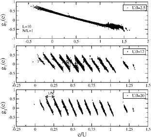
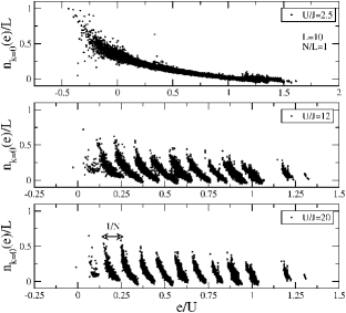
We here focus on the comparison of observables obtained from different ensembles in the 1D BHM. The evolution of one local and one global observable as a function of the eigenstates energy per particle is given in Fig. 5 and 6. Each of these two observables are used separately in the literature so we here give results for both for completeness. The observables are the one-particle density-matrix, defined for a translationally invariant Hamiltonian as:

$$g_{r}(e)=\frac{1}{L}\sum_{i=1}^{L}\langle{\psi_{f}(e)}|{b_{i+r}^{{\dagger}}b_{i}}|{\psi_{f}(e)}\rangle\;,$$ (10)

where $\left|{\psi_{f}(e)}\right\rangle$ is the eigenstate of energy $e$. $g_{r}(e)$ is a local observable since, for a given $r$, it can be attributed to a subsystem. On the contrary, the momentum distribution $n_{k}$ integrates information from all distances and may be considered as a global quantity:

$$n_{k}(e)=\sum_{r=-L+1}^{L-1}e^{ikr}g_{r}(e)\;.$$ (11)

In Fig. 5 and 6, one observes that both $g_{1}(e)$ and $n_{k=0}(e)$ evolve smoothly in the superfluid regime ($U/J=2.5$). One also realizes that the largest fluctuations are found in the low-energy part of the spectrum, supporting the energetic argument for the finite size effects. If one were able to choose $\bar{e}$ in the bulk of the “superfluid” spectrum, one would possibly find agreement with ETH. However, for the finite size systems at hand, one cannot reach the bulk of the spectrum before the Mott lobes emerge with $\lambda$. As it was shown in Ref. Biroli2009, and here confirmed, the observables strongly vary within each Mott lobe. We now turn the nature of the distributions for different quenches and compare the results for $g_{r}$ obtained by the different ensembles. Fig. 7 and 8 gather the data for a small and large quench from the superfluid region with $U_{i}=2$.

III.3.1 Small quench regime in the 1D BHM

Figure 7: (Color online) Comparison of different ensembles for different quenches. The effective temperature $T_{B}$ (given in Fig. 8) is fixed by the mean energy. The results are obtained on a system with $L=N=10$.

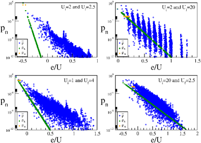
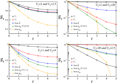
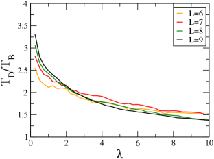
When $U_{f}=2.5$, the distribution is peaked on the final ground-state with a large weight $p_{0}$. The tail displays an exponential-like behavior that, however, has an effective temperature $T_{D}$ different from $T_{B}$, determined from the energy. This is easily understood from the fact that only the very few first weights significantly contribute to the energy, and they are not aligned with the tail. As $\bar{e}$ is very close to $e_{0,f}$ in this regime and as there are only a very few energies at the bottom of the spectrum, the microcanonical ensemble gives a bad mean energy and has only a few number of eigenstates. In this regime where $p_{0}$ is close to one, a minimal microcanonical ensemble would simply be $\left|{\psi_{0,f}}\right\rangle\left\langle{\psi_{0,f}}\right|$, although it has no statistical meaning. Looking at the correlations $g_{r}$ in Fig. 8 shows that they seem to be thermalized in the sense that $\rho_{B}$ gives a reasonable account of the correlations. However, $\left|{\psi_{0,f}}\right\rangle\left\langle{\psi_{0,f}}\right|$ also gives a reasonable account for the correlations while $\rho_{M}$ does not satisfactorily reproduce them. The system is in a regime dominated by finite size effects, far below the crossover number of bosons. The points of Ref. Kollath2007, in the “thermalized” region of the phase diagram seem to belong to this regime dominated by finite size effects. We have also looked at a slightly larger quench amplitude with $U_{i}=1$ and $U_{f}=4$ as in Fig. 3 of Ref. Kollath2007, (however, we work on a slightly smaller system size and the data displayed in Ref. Kollath2007, were averaged over time, so correlations cannot be quantitatively compared). Since $p_{0}$ is smaller, there is a substantial difference between the correlations in the final ground-state $U_{f}$ and the one from the diagonal ensemble. The canonical ensemble still gives the best agreement with $\bar{\rho}$. In a sense, the shape of the distributions as given in Ref. Roux2009, does explain the observation of Ref. Kollath2007, . Yet, the distribution is clearly not a true Boltzmann one as the temperature obtained from the mean energy and other observables are not identical. In order to investigate this deviation, or difficulty to define an effective temperature, we have computed the ratio between the two effective temperatures $T_{D}$ and $T_{B}$ in Fig. 9. For $L=6$ to 9, it remains between 1 and 3.5 and has a tendency to diverge at small quenches. Consequently, ETH does not apply here due to the presence of strong finite size effects, but one cannot claim either that the system is thermalized even though some correlations look thermalized in the canonical ensemble. The observed distributions are specific to this model and to these system lengths and parameters. We also point out that a similar regime has been observed in Ref. Rigol2009, , corresponding to low effective temperatures, but for which the diagonal ensemble distributions were not plotted.

Figure 8: (Color online) Comparison of averaged correlations $g_{r}$ corresponding the parameters of Fig. 7.

Still, the behavior of large systems ($N\geq N_{c}$) in the small quench regime remains an open but very interesting question as the low-energy physics will control the behavior. In this respect, we draw an argument in favor of non-thermalization: for symmetry reasons, the quench only excites states in the ground-state symmetry sector while the statistical ensembles average over all symmetry sectors. For instance, a system with a branch of excitation $E(k)$ can have a $k=0$ gap while the whole spectrum is gapless, hence it could not look thermalized. Starting from a finite temperature state or including symmetry breaking terms, like disorder, could partially cure this symmetry constraint.

Figure 9: (Color online) Ratio of effective canonical temperatures obtained from the distribution ($T_{D}$) and from the mean energy ($T_{B}$). Results are obtained for a quench starting at $U_{i}=2$.

III.3.2 Large quench regime

Results for two large quenches at a commensurate density $n=1$, from the superfluid parameters to deep into the Mott limit and reversely, are given in Fig. 7 and Fig. 8. For the first one, from $U_{i}=2$ to $U_{f}=20$, the distribution shows very strong fluctuations of the weights within each Mott lobes Roux2009 . In particular, large weights are present in the low-energy part of the first sub-bands. In Ref. Biroli2009, , it was shown that the larger values of $g_{1}$ were correlated to the larger weights (see another example of such a plot for an incommensurate density in Fig. 11), explaining that the ETH does not apply in these finite size systems. This is confirmed by looking at the time-averaged correlations that are neither reproduced by $\rho_{M}$ nor by $\rho_{B}$. DMRG calculations Kollath2007 ; Biroli2009 gave evidence that a non-thermal correlations $g_{r}$ survive for system sizes of order 100.

We now elucidate the origin of the observed non-thermalized regime, first by looking at the effect of the commensurability of the density in order to determine whether the presence of an equilibrium critical point plays a role for large quenches. As shown in Fig. 10 and 11, the phenomenology is very similar to the commensurate case with a non-thermalized regime at large quenches, except that there is no gap above the ground-state. Quenches that remain in the superfluid region (data not shown) also have the same behavior as for the commensurate case. These results suggest that the reason for non-thermalization is not related to the features of the low-energy spectrum, i.e. to the presence of a gap above the ground-state, but is related to the proximity of the $U=\infty$ limit of the model. However, in the small quench regime where the low-energy part of the spectrum governs the out-of-equilibrium physics, the opening of a gap can certainly play a role. Unfortunately, due to the finite size effects discussed in this paper, this interesting question cannot be addressed with reliability. For instance, it has been shown recently Li2009 that a quench in the quantum Ising model, which is integrable, is sensitive to the presence of the critical point. We note that the lobes could be qualitatively interpreted as stemming from a 1D gapped single-particle dispersion relation both in the commensurate and incommensurate regimes. However, in the latter case, there will not be any transition to an insulating state as a function of temperature.

Figure 10: (Color online) Quench from $U_{i}=2$ to $U_{f}=20$ for an incommensurate density $n=2/3$ for which there is no equilibrium quantum critical point. The structure of the density of states, the evolution of the local correlations $g_{r}$ and the shape of the distributions are very similar to the commensurate case.

One can actually argue that the large-$U$ structure of the distribution is reminiscent of the atomic limit $U=\infty$ in which we show that both the weights and the observables fluctuate and are correlated so that ETH is violated in this limit. What one can show is that the weights of a quench from $U_{i}=0$ to $U_{f}=\infty$ depend on the configuration in each of the degenerated Mott peaks of the $U_{f}=\infty$ limit. This argument does not rely on the $n=1$ commensurability condition. Indeed, the eigenstates of the final Hamiltonian are simply the set of configurations $\{n_{j}\}_{j=1,L}$ with $n_{j}$ the onsite occupations. The energy per particle of the configuration is

$$\frac{e(\{n_{j}\})}{U_{f}}=\frac{1}{2N}\sum_{i=j}^{L}n_{j}(n_{j}-1)\;.$$

The initial ground-state is the superfluid state that has equal single-particle probabilities $\mathfrak{p}_{j}=1/L$ on each site. Using formula (4), we get for the diagonal weights:

$$p_{n}=p_{\{n_{j}\}}=\frac{N!}{n_{1}!n_{2}!\cdots n_{L}!}\frac{1}{L^{N}}\;.$$ (12)

This makes a connection to the free boson model that we also study, having the $U_{f}$ energy spacing between the degenerate levels instead of $\hbar\omega_{f}$ and a different energy-configuration relation. The formula is valid for bare configurations, i.e. when they are not symmetrized. Using symmetries, formula (12) picks up an additional factor depending on the degeneracy of the generalized Bloch state. One can see by taking an example of two configurations with the same energy, or check numerically, that the weights can be different for configurations with the same energy, in the same way as for the free boson model. Consequently, in a strongly degenerate Mott peak, the diagonal weights are not equal and fluctuate. As soon as a non-integrable perturbation (here the hopping $J$) is turned on and lifts the degeneracy, the distribution of the weights will still strongly fluctuate within the Mott lobe. This explains the findings of Refs. Roux2009, ; Biroli2009, and of Fig. 7. Another simple observation in this limit is that two degenerate configurations can have different expectation values for the observables. An obvious one is the onsite particle distribution that counts empty, single, double occupations and so on. The off-diagonal correlation $g_{r}$ can be non-zero if the configurations are symmetrized and one can check numerically that they actually strongly differ for degenerate states. Notice that, in principle, one has to take into account the off-diagonal part of the time-averaged density-matrix that is non-zero in this highly degenerate limit. When one turns on $J$, this off-diagonal part vanishes and the $g_{r}$ still fluctuate strongly for eigenstates close in energy. Lastly, the asymmetrical correlation between the weights $p_{n}$ and the observables is also observed in this limit. We show this numerically on a system with $U_{i}=0$ and $U_{f}=100$ in Fig. 11 (we take $U_{f}/J=100$ and not $J_{f}=0$ because one needs a finite, yet very small, $J$ to make $\bar{\rho}$ diagonal). The numerics for a small $J/U$ in Fig. 7 and Fig. 5 strongly supports this mechanism as an explanation for the behavior of both the distributions and the observables. We remark that the argument works as well for the 2D version of the model that was shown to have a non-thermalized regime too Kollath2007 . The fate of this explanation in the thermodynamical limit is yet an open question. A scenario could be that this mechanism works above a certain critical quench amplitude $\lambda_{c}(N)$ but how this critical value behaves as $N\rightarrow\infty$ remains a difficult question. Consequently, one may understand the finite size effects stemming from the large-$U$ limit as another $N_{c}(\lambda)$ line in Fig. 3 increasing with $\lambda$ and that is specific to this model. Yet, non-thermalization in the thermodynamical limit in the BHM cannot be excluded as well. Experiments in cold atoms Greiner2002 work with a relatively small number of atoms and can easily reach this large-$U$ limit so that such considerations are physically relevant.

Figure 11: (Color online) Upper panel: comparison of the different observables in different ensembles (same parameters as in Fig. 10). Middle panel: the $p_{n}$ vs $g_{1}(n)$ curve gives proof of the non-relaxation towards a thermal state for the same parameters as in the upper panel. Lower panel: same plot but for the “integrable” quench limit $U_{i}=0$ and $U_{f}=100$.

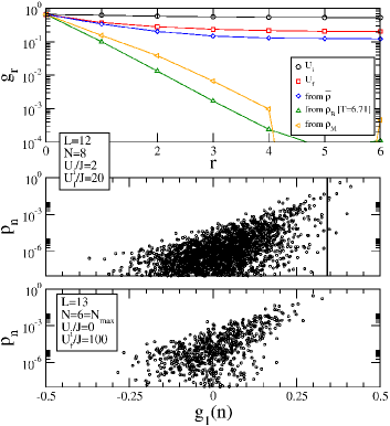
We also give results for a quench from the Mott to the superfluid limit. There, one could expect from Fig. 5 and  6 that ETH could work since the observables behave smoothly with $e$ in the final Hamiltonian. However, for the accessible sizes, one observes that the Boltzmann law still work better than the microcanonical ensemble, with large weights at low energies. We conclude that the breakdown of the ETH could here be attributed to finite size effects.

III.3.3 Free boson model

Figure 12: (Color online) Evolution of the distribution times the density of states of the diagonal ensemble for free bosons in an harmonic trap as a function of the quench amplitude. Here, the $p_{n}$ are the sum of the diagonal weights in each highly degenerate excitation sector.

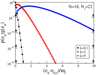
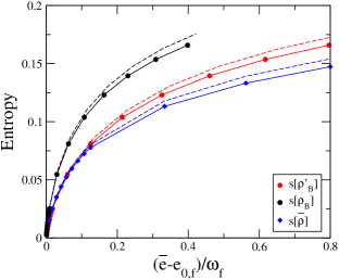
We now briefly discuss the evolution of the distribution for the free boson model for a fixed number of bosons and increasing $\lambda$. Very surprisingly, the distribution of the single-particle weights versus single-particle energies $\varepsilon_{2n}=2n\hbar\omega_{f}+\hbar\omega_{f}/2$ has some remarkable features (we recall that only the even levels can be occupied from symmetry reasons). In the limit of large energy $\varepsilon\sim 2n$, we have

$$\mathfrak{p}_{2n}\simeq\mathfrak{p}_{0}(\lambda)\frac{e^{-2n\ln|{\frac{\lambda+2}{\lambda}}|}}{\sqrt{\pi 2n}}\propto\frac{e^{-\varepsilon/T(\lambda)}}{\sqrt{\varepsilon}}$$

which has an exponential tail with the effective temperature $T(\lambda)=\hbar\omega_{f}/\ln\left|{\frac{\lambda+2}{\lambda}}\right|$. In the limit of small quenches, the distribution is Boltzmann-like with a temperature $T(\lambda)\simeq-\hbar\omega_{f}/\ln|\lambda/2|$ going to zero. This exponential-like behavior is not generic and a simple counter-example can be found in the case of an expanding box Aslangul2008 . For the many-particle situation with $N=18$ and $N_{s}=22$, we give in Fig. 12 the evolution of the distribution for increasing $\lambda$. For small quench, the behavior looks like Boltzmann (we do not expect a pure exponential law due to the presence of the degeneracy function $g(e)$, see below for a quantitative comparison) and it can be understood from the fact that the main contribution comes from single-boson excitations that have the same weights as the single-particle ones. When $\lambda$ is increased, the energy distribution gets peaked around a low-energy level and is strongly anisotropic with the maximum at a different place from the mean energy. This distribution finally develops a high-energy tail for large $\lambda$. One can compute analytically the third moment $M_{3}={\rm Tr}(\bar{\rho}(\mathcal{H}-\bar{E})^{3})$ which is non-zero and scales as $N$ showing that the distribution remains anisotropic and that the anisotropy $(M_{3})^{1/3}/(\bar{E}-E_{0,f})$ decreases as $N^{-2/3}$. In order to compare the distributions from different ensembles, we use the von-Neumann entropy of a density-matrix $\rho$ which is defined as $S_{vN}(\rho)=-\textrm{Tr}[\rho\ln\rho]$. Contrary to observables, this quantity is more sensitive to the tail of the distribution. $S_{vN}/N$ for the Boltzmann and diagonal ensembles are shown in Fig. 13. The density-matrix $\rho_{B}^{\prime}$ is a Boltzmann distribution but restricted to the even parity levels only. We see that for small quenches, $s(\rho_{B}^{\prime})$ and $s(\bar{\rho})$ are very close. The larger entropy for $s(\rho_{B})$ is simply due to the fact that half of the Hilbert space is not accessible to $\bar{\rho}$ for symmetry reasons: $s(\rho_{B}^{\prime})$ and $s(\rho_{B})$ are actually the same up to a factor 2 in the energy. Comparing the data to the microcanonical entropy is not relevant here because of finite size effects (energy discretization and small degeneracy of the first levels) for the values of the mean energy accessible here.

Figure 13: (Color online) Von Neumann entropy per particle versus energy for the free boson model. Dashed lines are data for $N=17$, full lines for $N=18$ ($N_{s}=22$).

IV Conclusions

The first conclusion we would like to highlight is that, when carrying out numerical simulations on a finite system, one has to care both about the quench amplitude and the size of the system to see in which region of the spectrum are the main weights of the diagonal ensemble distribution. It has been shown that, although the low-energy part of the spectrum is the place where the most interesting physics is expected, one experiences large finite size effects when exploring it. A crossover number of particles, distinguishing between the small quench regime and the large quench regime, can be tentatively defined from energetic considerations or from the static fidelity between the ground-states of the initial and final Hamiltonians. One advantage is that they can be computed numerically with few finite size effects (for the energy based criteria) or with ground-state techniques that work on larger systems (for both criteria). The numbers have been computed for the two models under study. As the system follows a finite size crossover between the two regimes, it can actually happen to be difficult for nowadays numerics to be close enough to the thermodynamical limit, where ETH is expected to work generically, even though some examples can be found in the literature Rigol2008 . This actually is what happens for the one-dimensional Bose-Hubbard model as we have seen. Hence, the thermalization-like regime in the small quench limit deduced from observables comparison and the qualitative Boltzmann-like structure of the distribution cannot be considered as truly thermalized because of dominant finite size effects. Furthermore, sizes accessible with full diagonalization cannot reach the bulk of the energy spectrum before the structure of the spectrum resembles the infinite-$U$ atomic limit. The free boson model nicely illustrates the crossover from a Boltzmann-like distribution, up to phase space constraints, at small quench to a different distribution. We note that due to the large density of states and to negligible energy fluctations, we may expect the quench, canonical and microcanonical distributions to eventually be equivalent in the thermodynamical limit. However, we have discussed the fact that the smaller the mean-energy (or equivalently the temperature), the larger are finite-size effects. We do not believe that the observed finite-size and canonical-like distributions at small quenches are generic (notice that no claim in that direction was made in Ref. Roux2009, ) and they may better be simply understood as (counter-)examples.

The second important conclusion is that we have shown that the non-thermalized regime observed on finite systems for large quenches in the 1D Bose-Hubbard model is actually related to the proximity of the $U=\infty$ atomic limit, something that may qualitatively be equivalent to the proximity of an integrable point. Indeed, this regime does not depend on the low-energy features at a commensurate density, i.e. to the presence of the superfluid-Mott transition, and besides, the structure of the diagonal ensemble stems from the $U=0\rightarrow U_{f}=\infty$ quench limit of the Bose-Hubbard model. In non-integrable models, the challenging issues on what are the features of the small quench regime for very large sizes and how the non-thermalized regime neighboring an integrable point survive in the thermodynamical regime seem to be hardly accessible to current numerical algorithms.