Thermodynamics of multiferroic spin chains

Abstract

The minimal model to describe many spin chain materials with ferroelectric properties is the Heisenberg model with ferromagnetic nearest neighbor coupling $J_{1}$ and antiferromagnetic next-nearest neighbor coupling $J_{2}$. Here we study the thermodynamics of this model using a density-matrix algorithm applied to transfer matrices. We find that the incommensurate spin-spin correlations - crucial for the ferroelectric properties and the analogue of the classical spiral pitch angle - depend not only on the ratio $J_{2}/|J_{1}|$ but also strongly on temperature. We study small easy-plane anisotropies which can stabilize a vector chiral order as well as the finite-temperature signatures of multipolar phases, stable at finite magnetic field. Furthermore, we fit the susceptibilities of LiCuVO₄, LiCu₂O₂, and Li₂ZrCuO₄. Contrary to the literature, we find that for LiCuVO₄ the best fit is obtained with $J_{2}\sim 90$ K and $J_{2}/|J_{1}|\sim 0.5$ and show that these values are consistent with the observed spin incommensurability. Finally, we discuss our findings concerning the incommensurate spin-spin correlations and multipolar orders in relation to future experiments on these compounds.

I Introduction

A number of spin-$1/2$ chain materials has recently been investigated in much detail which show multiferroic behavior, i.e., an intricate interplay of magnetic and electric order.Masuda et al. (2004); Park et al. (2007); Seki et al. (2008); Drechsler et al. (2007); Enderle et al. (2005); Büttgen et al. (2007); Schrettle et al. (2008) A microscopic model for the electric ordering based on a spin current mechanism has been introduced in Ref. Katsura et al., 2005 and seems to provide an understanding for most of the experimental findings. Here the electric polarization $\boldsymbol{P}$ is related to non-collinear spin-spin correlations, $\boldsymbol{P}\sim\boldsymbol{e}_{ij}\times(\boldsymbol{S}_{i}\times\boldsymbol{S}_{j})$, where $\boldsymbol{S}_{i}$ is a spin-$1/2$ operator at site $i$ and $\boldsymbol{e}_{ij}$ a vector connecting the chain sites $i$ and $j$. Later it has been shown based on a Ginzburg-Landau theory Mostovoy (2006) and symmetry arguments Kaplan and Mahanti (2008) that this coupling between the polarization and magnetization always exists independent of the crystal symmetry. To obtain a non-collinear spin structure on a lattice without geometrical frustration, a minimal model has to contain additional interactions apart from the nearest neighbor Heisenberg interaction. One possibility are frustrating longer range interactions. For chain materials consisting of edge sharing copper-oxygen plaquettes like LiCuVO₄, LiCu₂O₂ or Li₂ZrCuVO₄ the next-nearest neighbor interaction is particularly relevant leading to the minimal model

$$H=\sum_{r}\left\{J_{1}(\boldsymbol{S}_{r}\boldsymbol{S}_{r+1})_{XXZ}+J_{2}(\boldsymbol{S}_{r}\boldsymbol{S}_{r+2})_{XXZ}-hS^{z}_{r}\right\}.$$ (1)

Here $(\boldsymbol{S}_{r}\boldsymbol{S}_{r+i})_{XXZ}=S^{x}_{r}S^{x}_{r+i}+S^{y}_{r}S^{y}_{r+i}+\Delta S^{z}_{r}S^{z}_{r+i}$ with $\Delta\leq 1$ being an exchange anisotropy. For the edge sharing chains the nearest neighbor coupling is ferromagnetic ($J_{1}<0$) while the next-nearest neighbor coupling is antiferromagnetic ($J_{2}>0$). This is the case we want to study here. The external magnetic field is denoted by $h$. In the classical isotropic model ($\Delta=1$) without field the frustration leads to a helical spin arrangement with a pitch angle $\phi=\arccos(1/4\alpha)$ for $\alpha=|J_{2}/J_{1}|>1/4$. As in the classical model, the ground state of the quantum model (1) is ferromagnetic for $\alpha<1/4$. For $\alpha>1/4$ the ground state is a singlet whose nature has not fully been clarified yet.White and Affleck (1996); Itoi and Qin (2001) Based on a renormalization group treatment starting from two decoupled Heisenberg chains ($J_{1}=0$), it has been predicted that any small $J_{1}<0$ produces a finite but tiny excitation gap.Itoi and Qin (2001) Numerically such a gap could not be resolved so far.

Due to the $SU(2)$ spin rotational symmetry only a quasi long-range helical order (algebraically decaying) is possible in the isotropic model (1) without field. Whether the correlation functions are indeed algebraically or instead exponentially decaying with a very large correlation length as suggested in Ref. Itoi and Qin, 2001 is a question which we will not address here and which is not important for the following discussions. One can in any case still define a pitch angle $\phi$ by studying the spin-spin correlation functions which, however, turns out to be substantially modified compared to the classical case due to quantum fluctuations.Bursill et al. (1995) If the $SU(2)$ symmetry is broken by applying either a magnetic field $h$ or by an anisotropy $\Delta<1$ then the vector chirality

$$\kappa^{(n)}=(\boldsymbol{S}_{r}\times\boldsymbol{S}_{r+n})^{z}=\frac{i}{2}(S^{+}_{r}S^{-}_{r+n}-S^{-}_{r}S^{+}_{r+n})$$ (2)

can have a nonzero expectation value because this requires only the breaking of the remaining $\mathbb{Z}_{2}$ symmetry. The vector chirality as defined in (2) is directly related to the spin current $j_{r}=j_{r}^{(1)}+j_{r}^{(2)}$ which can be obtained from a continuity equation $\partial_{t}S^{z}+\partial_{r}j=0$. The equation of motion yields $\partial S^{z}_{r}=i[H,S^{z}_{r}]=-J_{1}(\kappa_{r}^{(1)}-\kappa_{r-1}^{(1)})-J_{2}(\kappa_{r}^{(2)}-\kappa_{r-2}^{(2)})$ which leads to the indentification $j=J_{1}\kappa^{(1)}+2J_{2}\kappa^{(2)}$.Hikihara et al. (2008)

It has been shown recently that a magnetic field can also stabilize multipolar phases apart from a phase with chiral order, both in the isotropic as well as in the anisotropic case.Heidrich-Meisner et al. (2009); Sudan et al. (2008); Hikihara et al. (2008); Furukawa et al. (2008) Such multipolar phases are characterized by short-range transverse spin correlations $\langle S^{+}_{0}S^{-}_{r}\rangle$ while correlations functions $\langle\underbrace{S^{+}_{0}S^{+}_{1}\cdots}_{\tiny\mbox{n times}}\underbrace{S^{-}_{r}S^{-}_{r+1}\cdots}_{\tiny\mbox{n times}}\rangle$ are algebraically decaying in an $n$-polar phase.

In this article we want to investigate how the spin-spin correlations of the $J_{1}$-$J_{2}$ model (1) are affected not only by quantum but also by thermal fluctuations. At the end we want to relate our numerical results with various experiments on edge sharing copper-oxygen chains. A very powerful numerical method to study the thermodynamics of one-dimensional quantum chains directly in the thermodynamic limit is the density-matrix renormalization group applied to transfer matrices (TMRG). Here the Hilbert space is truncated to a small fixed number of states while the temperature is lowered successively. In the calculations presented here we will typically retain $N=60-200$ states both in the system and the environment block. We will present data for temperatures where the algorithm seems to be converged which is judged by comparing results obtained for different numbers of states. For a detailed description of the TMRG algorithm the reader is referred to Refs. I.Peschel et al., 1999; Sirker and Klümper, 2002a, b; Glocke et al., 2008. In a previous TMRG study the isotropic $J_{1}$-$J_{2}$ model was investigated, however, correlation functions were not calculated.Lu et al. (2006)

The manuscript is organized as follows: In Sec. II we study the isotropic model without magnetic field paying special attention to the evolution of the incommensurabilities with temperature. In Sec. III we consider the experimentally relevant case of a small easy-plane anisotropy. In Sec. IV we investigate signatures of multipolar phases, which are stable for finite magnetic field, at finite temperatures. Finally, in Sec. V, we relate our numerical results to data for three experimentally well studied compounds (LiCuVO₄, LiCu₂O₂, Li₂ZrCuVO₄). In particular, we fit the susceptibilities using model (1) which allows us to extract the parameters $J_{1}$ and $J_{2}$. We also discuss neutron scattering experiments which give access to the pitch angle and suggest future experiments regarding the realization and observation of multipolar orders. The last section is devoted to a brief summary and some conclusions.

II Thermodynamics of the $J_{1}$-$J_{2}$ chain

For the isotropic case, $\Delta=1$, without magnetic field it is known that there is a quantum critical point at $\alpha=1/4$ separating a ferromagnetic phase for $\alpha<1/4$ from a phase with a singlet ground state. A tiny gap for $\alpha>1/4$ has been predicted,Itoi and Qin (2001) however, even if this gap really exists it will only show up at extremely low temperatures. In the temperature range accessible numerically, the susceptibility $\chi$ for $\alpha\to\infty$ smoothly approaches the result for the nearest-neighbor Heisenberg chain known from Bethe ansatz Klümper (1993) as is shown in Fig. 1.

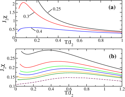
Figure 1: (color online) (a) Susceptibilities near the quantum critical point $\alpha=1/4$. (b) Susceptibilities for $\alpha=2.0,\,1.6,\,1.2,\,1.0,\,0.8,\,0.6$ (solid lines from bottom to top). For comparison, the result for the nearest-neighbor Heisenberg chain obtained by Bethe ansatz is shown (dashed line).

At the critical point, $\chi(T)$ will show a power-law divergence.Härtel et al. (2008) A thorough investigation of the critical properties using the TMRG algorithm will be presented elsewhere.Nishimoto et al. (2009)

Numerically, we can also obtain the inner energy $e$ and the free energy $f$ (see Ref. Glocke et al., 2008). This gives us the entropy $s=(e-f)/T$ and the specific heat $C=T\partial s/\partial T$ using a numerical derivative. The results for various $\alpha$ are presented in Fig. 2.

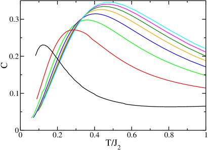
Figure 2: (color online) Specific heat for $\alpha=0.4,0.6,\cdots,2.0$ (from bottom to top).

For all frustration parameters we find a broad maximum which shifts monotonically to larger temperatures $T/J_{2}$ with increasing $\alpha$.

Next, we want to study various correlation functions. At finite temperatures all correlation functions will be exponentially decaying and we can expand any two-point correlation function of an operator $O_{r}$ as

$$\langle O_{0}O_{r}\rangle-\langle O_{0}\rangle\langle O_{r}\rangle=\sum_{j=0}^{\infty}M_{j}\text{e}^{-r/\xi_{j}}\cos(k_{j}r)\;.$$ (3)

Here $M_{j}$ is a matrix element, $\xi_{j}$ a correlation length, and $k_{j}$ the corresponding wave vector. Within the TMRG algorithm both $\xi_{j}$ and $k_{j}$ are determined by the ratio of the leading to next-leading eigenvalues of the transfer matrix. I.Peschel et al. (1999); Glocke et al. (2008) For large distances $r\gg 1$ the correlation function is dominated by the largest correlation length and the corresponding wave vector which we will denote as $\xi\equiv\xi_{0}$ and $k\equiv k_{0}$ in the following.

Of particular interest is the evolution of the wave vector $k$ for the spin-spin correlation $\langle\boldsymbol{S}_{0}\boldsymbol{S}_{r}\rangle$. This can be seen as the quantum mechanical analogue of the pitch angle of the classical spiral. In Fig. 3 it is shown that $k$ does not only depend on the frustration $\alpha$ but also shows a strong dependence on temperature, in particular, for values of $\alpha$ close to the critical point $\alpha_{c}=1/4$.

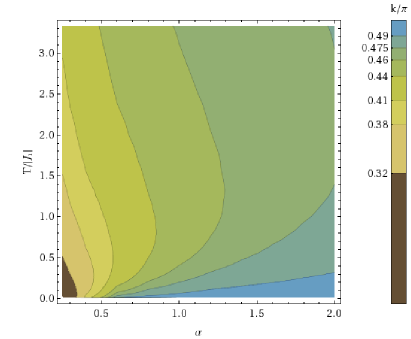
Figure 3: (color online) The wave vector $k$ of the spin-spin correlation function depends not only on $\alpha$ but also on temperature. With increasing temperature, $k$ first increases for $\alpha$ close to $\alpha_{c}$ while it decreases for larger $\alpha$.

Contrary to the classical case, the pitch angle at low temperatures is very close to $\pi/2$ for $\alpha\gtrsim 0.6$ as is shown in more detail in Fig. 4(a).

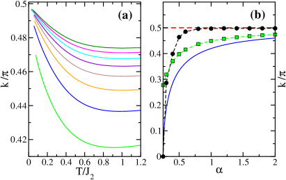
Figure 4: (color online) (a) $k$ as a function of temperature for $\alpha=0.6,0.8,\cdots,2.0$ (from bottom to top). (b) Extrapolated $k$ (pitch angle) for zero temperature (circles), and $k$ at $T/J_{2}=1.0$ (squares). The dashed lines are a guide to the eye. For comparison, the classical pitch angle $\phi=\arccos(1/4\alpha)$ (solid line) is shown.

This means that for these frustration values the spin structure develops an almost perfect (short-range) four-site periodicity at low temperatures. In Fig. 4(b) the extrapolated $k$ value (pitch angle) for zero temperature is shown as a function of $\alpha$. Our result is in good agreement with an earlier DMRG calculation.Bursill et al. (1995) We also find that with increasing temperature the pitch angle becomes again more classical for a frustration $\alpha\gtrsim 0.5$ (see squares in Fig. 4(b)).

One might think that the strong trend towards a formation of a four-site periodic structure with increasing $\alpha$ could be related to a concomitant dimerization. However, as is shown exemplarily in Fig. 5, this is not the case.

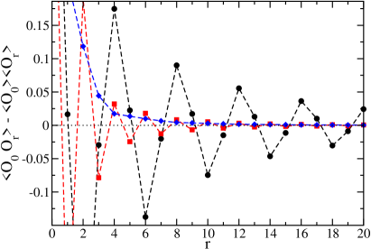
Figure 5: (color online) Various correlation functions for $\alpha=2$ and $T/J_{2}=0.05$. The circles denote the spin-spin ($O_{r}=\boldsymbol{S}_{r}$), the squares the dimer ($O_{r}=\boldsymbol{S}_{r}\boldsymbol{S}_{r+1}$), and the diamonds the chiral correlation function ($O_{r}=\boldsymbol{S}_{r}\times\boldsymbol{S}_{r+1}$). The lines are a guide to the eye.

While substantial dimer and chiral correlations with comparable correlation lengths do exist, both correlation lengths are about a factor $2$ smaller than the spin-spin correlation length.

Another way of defining a quantum analogue of the classical pitch angle is the possibility to study at which wave vector $q$ the static spin structure factor

$$S(q)=\frac{3}{4}+2\sum_{r=1}^{\infty}\cos(q\,r)\langle\boldsymbol{S}_{0}\boldsymbol{S}_{r}\rangle$$ (4)

is peaked. This definition of the pitch angle is equivalent to the definition in (3) if the correlation function is dominated by the leading correlation length, i.e., $\xi_{0}\gg\xi_{j}$ for $j\geq 1$. This is the case for all frustration parameters shown in Fig. 6 except for the critical value $\alpha_{c}=1/4$ (Fig. 6(a)).

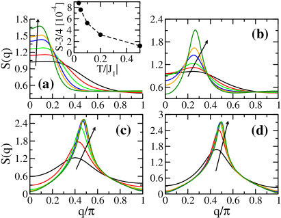
Figure 6: (color online) The static spin structure factor $S(q)$ for temperatures $T/|J_{1}|=0.5,0.2,0.1,0.05,0.035,0.02$ (along the arrow direction) with (a) $\alpha=1/4$ (quantum critical point), (b) $\alpha=0.3$, (c) $\alpha=0.6$, and (d) $\alpha=1.0$. The inset of (a) shows the deviation from the sum rule $S\equiv\sum_{q}S(q)=3/4$.

Here the structure factor is very flat near $q\sim 0$ meaning that in the expansion (3) comparable correlation lengths exist with a wave vector $k=0$ and with wave vectors which have small incommensurate values. The accuracy of the numerical data can be checked by calculating the sum rule. For all $\alpha$ and all temperatures the sum rule is fulfilled with deviations of the order $10^{-3}$ to $10^{-4}$ as is exemplarily shown in the inset of Fig. 6(a).

III The anisotropic case

In the edge-sharing spin chain compounds substantial exchange anisotropies exist. For LiCuVO₄, for example, the $g$ tensor has been measured by ESR and an exchange anisotropy of the order of $6\%$ percent has been estimated.Krug von Nidda et al. (2002) This anisotropy is expected to pin the spins to the $ab$ plane and this is indeed observed in experiment.Enderle et al. (2005); Schrettle et al. (2008) Theoretically, one expects that an $XXZ$-type anisotropy ($\Delta\lesssim 1$) enhances chiral correlations. In this case even long range chiral order ($\langle\kappa^{(n)}\rangle\neq 0$) is possible at zero temperature in the purely one-dimensional model because only the remaining $\mathbb{Z}_{2}$ symmetry has to be broken. In previous numerical studies the anisotropic model (1) has already been investigated, the results, however, have been contradictory.Somma and Aligia (2001); Furukawa et al. (2008) In Ref. Somma and Aligia, 2001 a large region of the phase diagram has been found to be occupied by a dimer phase whereas spin liquid phases occur for very small and large values of $\alpha$. In Ref. Furukawa et al., 2008 a dimer phase and spin liquid phases have again been found but in addition also a chiral phase for $\alpha\gg 1$. Both studies were based on exact diagonalization. In a very recent density-matrix renormalization group study the anisotropic model at finite magnetization was investigated.Heidrich-Meisner et al. (2009) A dimer phase was not found to be stable, instead it was shown that for most parameters a chiral phase or a spin liquid phase (SDW₂ phase) occur.

We will first concentrate on one value of anisotropy, $\Delta=0.8$. This is larger than what is expected for the edge-sharing cuprate chains. However, this way the effects of the anisotropy are more obvious and the results should qualitatively be similar to those for realistic values for these materials. We will study the case of zero field to see whether a dimer or a chiral phase occur. In Fig. 7 results for various correlation lengths at $\alpha=0.4$ are shown.

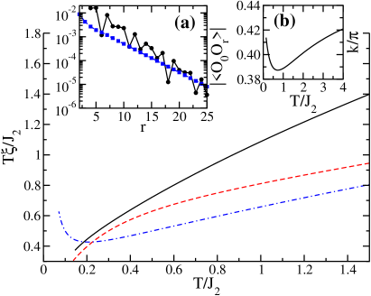
Figure 7: (color online) The longitudinal spin (solid line), dimer (dashed line), and chiral correlation length (dot-dashed line) for $\alpha=0.4$ and $\Delta=0.8$. At low temperatures the chiral correlation length diverges stronger than $1/T$ indicating long-range order at zero temperature. (a) The longitudinal spin-spin and the chiral correlation function at $T/J_{2}=0.125$ showing that chiral correlations dominate. (b) The wave vector $k$ of the longitudinal spin-spin correlation function.

For correlation functions which decay algebraically at zero temperature we expect that the correlation length diverges as $\xi\sim 1/T$. Studying $\xi T$ as in Fig. 7 thus separates long and short ranged correlations. In this case we see that the chiral correlation length diverges stronger than $1/T$ indicating that for these parameters we do have long range chiral order at zero temperature. While the dimer is indeed larger than the chiral correlation length over a wide temperature range, the situation is reversed at low temperatures. Hence a dimer phase can only possibly occur if also interchain couplings are present which might stabilize such an order at intermediate temperatures. That the chiral correlations indeed dominate at low temperatures is shown exemplarily for $T/J_{2}=0.125$ in Fig. 7(a) where the chiral and longitudinal spin-spin correlation functions are compared. Here the wave vector $k$ of the longitudinal spin-spin correlation function is incommensurate and again shows a strong dependence on temperature (Fig. 7(b)).

For $\alpha=0.6$, shown in Fig. 8(a), the chiral correlation length is again dominant at the lowest temperatures which are accessible numerically, however, there is no indication for long range chiral order at zero temperature. Remarkably, all three correlation lengths are of very similar magnitude at low temperatures. This suggest that we are very close or at the phase transition from a phase with long range chiral order at smaller values of $\alpha$ to a phase which most likely has spin liquid character with algebraically decaying correlation functions.

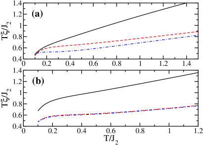
Figure 8: (color online) The longitudinal spin (solid line), dimer (dashed line) and chiral (dot-dashed line) correlation lengths for $\Delta=0.8$ with (a) $\alpha=0.6$ and (b) $\alpha=2.0$.

Indeed, at $\alpha=2.0$ shown in Fig. 8(b) the spin-spin correlation length is clearly dominant with oscillations $k\approx\pi/2$ at low temperatures pointing to an SDW₂ phase. We conclude that if a dimer phase exist at all for $\Delta=0.8$ it has to be confined to a very narrow range of frustration parameters $0.4<\alpha<0.6$. In Ref. Somma and Aligia, 2001 an unidentified phase was found for $0.3\lesssim\alpha\lesssim 0.45$ with symmetries as expected for the chiral phase. For $\alpha\gtrsim 0.7$, on the other hand, a spin liquid phase was predicted with a dimer phase in between these two phases. In our TMRG calculations we never find dominant dimer correlations at low temperatures and our results suggest that a dimer phase might not be stable at all but instead a direct phase transition from the chiral to a SDW₂ phase at $\alpha\approx 0.6$ occurs.

IV Finite magnetic field: Multipolar phases

In the multiferroic spin chain compounds a magnetic field can be used to switch the electric polarization. A sufficiently strong field induces a flop of the spins from the easy-plane spiral to a spiral perpendicular to the applied magnetic field. According to the spin current mechanism this also leads to a rotation of the electric polarization. Such a switching of the ferroelectric polarization by an applied magnetic field has been observed in LiCuVO₄ Schrettle et al. (2008) as well as in LiCu₂O₂.Park et al. (2007) Numerical studies of the $J_{1}$-$J_{2}$ model have shown that small magnetic fields stabilize the chiral order while multipolar phases become stable at intermediate field strengths before the system ultimately becomes fully polarized for large fields.Hikihara et al. (2008); Sudan et al. (2008); Furukawa et al. (2008)

As already eluded to in the introduction, an algebraic decay of the $\langle\underbrace{S^{+}_{0}S^{+}_{1}\cdots}_{\tiny\mbox{n times}}\underbrace{S^{-}_{r}S^{-}_{r+1}\cdots}_{\tiny\mbox{n times}}\rangle$ correlation function is expected in an $n$-polar ($n\geq 2$) phase while the transverse spin correlation function is gapped. For the oscillations of the longitudinal spin correlation function we expect in general

$$k_{T\to 0}=\frac{\pi}{n}(1-2m)$$ (5)

where $m$ is the magnetization and is directly related to the shift of the Fermi points. For zero field, $n=2$ would correspond to the $4$-site periodic spin structure discussed previously.

An particular interesting case is $\alpha=0.4$ with $h=0.25\,J_{2}$ shown in Fig. 9. Here we find that the longitudinal spin correlation length is largest at high temperatures, then there is a temperature range where the chiral correlation length dominates while at the lowest accessible temperatures the spin correlation again dominates and seems to diverge like $1/T$.

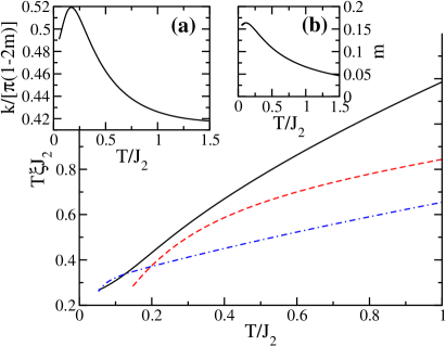
Figure 9: (color online) The longitudinal spin (solid line), dimer (dashed line) and chiral (dot-dashed line) correlation lengths for $\alpha=0.4$ with $\Delta=1$ and $h=0.25\,J_{2}$. (a) The wave vector $k$ of the spin-spin correlation. (b) The magnetization $m$ as a function of temperature.

For zero temperature this field corresponds to a magnetization $m\approx 0.15\approx 0.3m_{\rm sat}$ (Fig. 9(b)) where $m_{\rm sat}=0.5$ is the saturation magnetization. Comparing with the zero temperature phase diagrams obtained in Refs. Hikihara et al., 2008; Sudan et al., 2008 we see that for these values we are in the SDW₂ phase but very close to the phase boundary with the chiral phase. Our results basically seem to confirm this picture although the oscillations $k$ apparently slightly deviate from the value expected for a $n=2$ multipolar phase even at the lowest temperatures (see Fig. 9(a)). Our data also show that in a certain temperature window chiral correlations can still be dominant. This might be relevant once interchain couplings are taken into account and might lead to a chiral phase stable at intermediate temperatures while the spins are collinear at higher and lower temperatures. Two magnetic phase transitions have indeed been observed in LiCu₂O₂ where first a sinusoidal magnetic order is established followed by a helical order at lower temperatures.Park et al. (2007); A. Rusydi et al. (2008) While the magnetic structure even in the low temperature phase apparently is much more complicated than a simple planar spiralA. Rusydi et al. (2008) and the $J_{1}$-$J_{2}$ model does not seem to capture the essential physics of this compound (see next section) it is nevertheless interesting that even in this very simple model phases might be stable only in a certain temperature range thus possibly giving rise to multiple magnetic phase transitions once interchain couplings are taken into account.

In Fig. 10 the longitudinal spin structure factor $S^{zz}(q)$ is shown for $\alpha=0.32$ and $h=0.02J_{1}$.

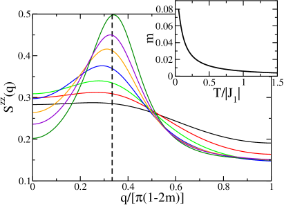
Figure 10: (color online) $S^{zz}(q)$ for $\alpha=0.32$, $h=0.02J_{1}$ and temperatures $T/|J_{1}|=2.0,1.0,0.5,0.2,0.1,0.07,0.05$ (from botom to top). The dashed line marks $q/[\pi(1-2m)]=1/3$. The inset shows the magnetization $m$ as function of temperature.

At low temperatures $S^{zz}(q)$ is peaked at $q=\pi(1-2m)/3$ (dashed line in Fig. 10) indicating an $n=3$ multipolar phase. Thus experimentally a multipolar phase can already be indentified at finite temperatures by studying the evolution of the structure factor as obtained in neutron scattering. Such an experiment would be most interesting for a compound close to the quantum critical point $\alpha_{c}=1/4$ where small magnetic fields are sufficient to stabilize $n=3$ or even $n=4$ multipolar phases.Sudan et al. (2008) As discussed in detail in Ref. Drechsler et al., 2007 and in the following section, Li₂ZrCuO₄ seems to be a very promising candidate for such a material.

V Multiferroic spin chain materials

While in the corner sharing copper-oxygen chain compounds like Sr₂CuO₃ and SrCuO₂ the antiferromagnetic exchange interaction is of very similar magnitude, $J\sim 2000$ K, a wide range of exchange parameters $J_{1}$ and $J_{2}$ can be found in the literature for the edge sharing compounds. For LiCuVO₄, for example, fits of the susceptibility and of neutron scattering data have led to the estimate $J_{1}\sim-20$ K and $J_{2}\sim 50$ K so that $\alpha\sim 2.5$.Enderle et al. (2005) For Li₂ZrCuO₄, on the other hand, susceptibility and specific heat data have been fitted by using $J_{1}\sim-300$ K and $\alpha\sim 0.3$.Drechsler et al. (2007) Given that the chains in these compounds consist of the same edge sharing copper-oxygen plaquettes, this huge variation in the magnitude of the exchange couplings is surprising.

Here we want to reanalyze the data of three of the best studied multiferroic chain compounds namely Li₂ZrCuO₄, LiCuVO₄ and Li₂CuO₂. We will concentrate on fitting susceptibility data using

$$\chi_{\rm exp}=\chi_{0}+\chi_{J_{1}-J_{2}}\;.$$ (6)

Here $\chi_{\rm exp}$ is the experimentally measured susceptibility, $\chi_{0}$ is a constant contribution due to core diamagnetism and Van-Vleck paramagnetism and $\chi_{J_{1}-J_{2}}$ is the numerically calculated susceptibility for the $J_{1}$-$J_{2}$ model (1). Such fits work extremely well for the corner sharing compounds because the intrachain coupling is about three orders of magnitude smaller than the interchain coupling.Motoyama et al. (1996); Eggert et al. (1994); Sirker et al. (2007, 2008); Sirker and Laflorencie (2009) For LiCuVO₄ it has been reported that a three-dimensional (3D) magnetic order becomes established below $T_{3D}\sim 2.3$ K.Büttgen et al. (2007) While this points to intrachain couplings which are only one or at most two orders of magnitude smaller than the interchain couplings, a purely one-dimensional model is still expected to be a good approximation as long as $T\gg T_{3D}$. In Li₂ZrCuO₄ the situation has not fully been clarified yet. A possible phase transition might occur at $T\sim 6$ K.Drechsler et al. (2007) Even if this is a 3D ordering transition, a one-dimensional model should again be valid over a wide temperature range. Therefore the expectation is that the physics of LiCuVO₄ and Li₂ZrCuO₄ can largely be understood within the framework of the $J_{1}$-$J_{2}$ model with the spin-current mechanism being responsible for the multiferroic properties.

The situation for LiCu₂O₂, on the other hand, seems to be much more involved.Masuda et al. (2004); Park et al. (2007); A. Rusydi et al. (2008); Seki et al. (2008); Huang et al. (2008) Despite a number of studies, the magnetic structure remains controversial. For instance, both a spiral spin order in the $ab$ as well as in the $bc$ plane have been reported.Masuda et al. (2004); Seki et al. (2008) If the spin current model is the correct explanation for the observed polarization along the $c$-axisPark et al. (2007) then the $bc$ spiral must be realized. The two magnetic ordering transitions at comparitatively large temperatures, $T\approx 22$ K and $T\approx 24$ K,A. Rusydi et al. (2008) point to much larger interchain couplings than for the two other compounds discussed above. In fact, it has been found that there are substantial spin correlations not only along the chain direction ($b$-axis) but also in the plane of the copper-oxygen plaquettes perpendicular to the chain direction ($a$-axis) making the compound at low temperatures almost two dimensional.Huang et al. (2008) One might speculate that the reason why the magnetic properties of this material are so different is related to the fact that two different copper sites exist - the in-chain Cu²⁺ and the Cu¹⁺ interconnecting different chains. This might lead to substantial charge fluctuations and thus to enhanced magnetic interchain couplings. Nevertheless, a fit of the susceptibility at high temperatures using the $J_{1}$-$J_{2}$ model might still be useful to obtain an estimate for the magnitude of the $J_{1}$ and $J_{2}$ couplings.

The absolute values of the measured maxima of $\chi$ already allow some general statements about the magnitude of the exchange constants and the frustration parameters $\alpha$. In LiCuVO₄ and in LiCu₂O₂ the susceptibility is about two orders of magnitude larger than in the corner sharing chain compounds Sr₂CuO₃ and SrCuO₂ so that the antiferromagnetic exchange constant $J_{2}$ should also roughly be two orders of magnitude smaller. In Li₂ZrCuO₄ the maximum is almost an order larger than in the other two compounds clearly indicating that this compound should be closer to the quantum critical point $\alpha_{c}=1/4$ than the other two compounds. If the magnetic exchange constants are of comparable magnitude, then $\alpha$ is expected to be largest for LiCu₂O₂ and smallest for Li₂ZrCuO₄ with LiCuVO₄ having an intermediate frustration parameter.

The susceptibility of LiCuVO₄ shown in Fig. 11 has a maximum and a local minimum at low temperatures. If $\chi$ can indeed be described by the $J_{1}$-$J_{2}$ model then a comparison with Fig. 1 indicates that $\alpha\sim 0.5$. The large $\alpha$ used in Ref. Enderle et al., 2005 can certainly not explain this structure. By performing a fit according to (6) we find that $J_{2}=91$ K and $\alpha=0.5$ yields the best fit as shown in Fig. 1(a). A good fit is also possible with $J_{2}=72$ K and $\alpha=0.6$ (Fig. 1(b)). If we reduce the next-nearest neighbor exchange to $J_{2}\sim 50$ K as assumed in Ref. Enderle et al., 2005 we have to choose $\alpha\sim 1$ to obtain the best fit possible with this value of $J_{2}$ (Fig. 1(c)). However, such a fit fails to reproduce the low temperature structure.

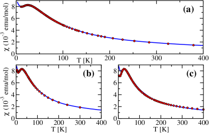
Figure 11: (color online) The experimentally measured susceptibility of LiCuVO₄ for $H\parallel c$ (solid line) compared to fits (dots) following Eq. (6) with a gyromagnetic ratio $g=2.313$.Büttgen et al. (2007); Krug von Nidda et al. (2002) (a) The best fit is obtained with $\chi_{0}=6\cdot 10^{-5}$ emu/mol, $J_{2}=91$ K, and $\alpha=0.5$. (b) An alternative fit with $\chi_{0}=1.4\cdot 10^{-4}$ emu/mol, $J_{2}=72$ K, and $\alpha=0.6$. (c) An exchange coupling $J_{2}=52$ K similar to the one in Ref. Enderle et al., 2005 can be used with $\chi_{0}=2.7\cdot 10^{-4}$ emu/mol, however, the frustration parameter $\alpha=1.0$ chosen to obtain the best fit is still much smaller than the one in Ref. Enderle et al., 2005 and the fit is much worse than the ones shown in (a) and (b).

The susceptibility data for Li₂ZrCuO₄ have already been analyzed in Ref. Drechsler et al., 2007 by comparing with exact diagonalization data for small rings consisting of up to $N=20$ sites. Finite size effects are expected to be neglegible if $T\gg v/N$ where $v$ is the spin velocity. The spin velocity is of the order of the exchange constant so that the finite size data for $\chi$ should be reliable for $T\gtrsim 20$ K. Given that the maximum of $\chi$ is located at $T\approx 7.6$ K, i.e., at temperatures where finite size effects might play a role, it is helpful to reanalyze the experimental data using the TMRG algorithm which yields results directly for the infinite system. As shown in Fig. 12 very similar fits to the one in Ref. Drechsler et al., 2007 are obtained.

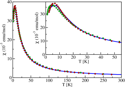
Figure 12: (color online) The measured susceptibility (solid line) for Li₂ZrCuO₄ taken from Ref. Drechsler et al., 2007 compared to fits using the $J_{1}-J_{2}$ model. An excellent fit (circles) is obtained using $\alpha=0.3$, $g=2$ and $J_{1}=-273$ K ($J_{2}=81.9$ K) with $\chi_{0}=0$ confirming the analysis in Ref. Drechsler et al., 2007 based on exact diagonalization data. A reasonable fit (squares) is also possible with $\alpha=0.4$, $g=2.2$, $\chi_{0}=0$, and $J_{1}=-75$ K. Inset: Blow-up of the low temperature region.

While the magnitude of the frustration parameter can only be varied slightly if one wants to obtain a reasonable fit, the exchange parameters change dramatically, for example, from $J_{1}=-273$ K for $\alpha=0.3$ to $J_{1}=-75$ K for $\alpha=0.4$. In LDA calculations $J_{1}=-151\pm 35$ K and $J_{2}=35\pm 12$ K was found which also will allow for a reasonable fit with a frustration parameter $\alpha\in[0.3,0.4]$.Drechsler et al. (2007) We therefore confirm the main conclusion of Ref. Drechsler et al., 2007 that Li₂ZrCuO₄ is close to the critical point $\alpha_{c}=1/4$.

Finally, we want to analyze the susceptibility data for LiCu₂O₂. As already mentioned, we do not expect that the $J_{1}$-$J_{2}$ model will describe the susceptibility of this compound at low temperatures and indeed we find that it is impossible to obtain a good fit down to low temperatures (see Fig. 13).

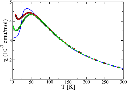
Figure 13: (color online) The measured susceptibility (solid line) for LiCu₂O₂ with $H\parallel c$ taken from Ref. Masuda et al., 2004 compared to fits using the $J_{1}-J_{2}$ model. With $g=2.2$ the best fit is obtained with $\alpha=0.6$, $J_{2}=120$ K and $\chi_{0}=0$ (circles) while for $g=2.3$ a fit with $\alpha=1.6$, $J_{2}=83$ K and $\chi_{0}=0$ works best (squares).

If we concentrate on temperatures large compared to the magnetic ordering transitions at $T\sim 20$ K, then a fit is possible and we find that $J_{2}\approx 80-120$ K. Because the susceptibility can only be fitted at high temperatures, the frustration parameter cannot be fixed precisely.

It is, however, important to note that the best fits for all three compounds yield values of $J_{2}\lesssim 100$ K while $J_{1}\sim-200$ K. This confirms our expectation that these materials consisting of the same edge sharing copper-oxygen plaquettes should have very similar magnetic exchange constants as is also the case for the corner sharing chain compounds. The values we obtain from the susceptibility fits are consistent with values in the literature for LiCu₂O₂ ($J_{1}\sim-120$ K, $J_{2}\sim 80$ K) Masuda et al. (2004); Park et al. (2007) and for Li₂ZrCuO₄.Drechsler et al. (2007) For LiCuVO₄, however, we find values which differ dramatically from the values given in Ref. Enderle et al., 2005 which later were also used in a number of other publications. We want to stress again that these values are not consistent with the latest susceptibility data.Büttgen et al. (2007) An analysis of neutron scattering data using a standard spin-wave dispersion which seems to confirm these values Enderle et al. (2005) is in our opinion not applicable here. In such an analysis the magnon bandwidth is directly determined by the bare exchange couplings while the stark deviation of the quantum from the classical pitch angle (see Fig. 4(b)) suggests that the frustration parameter is strongly renormalized due to quantum fluctuations.

The pitch angle measured experimentally in Ref. Enderle et al., 2005 of $\phi\approx 83.7^{\circ}$ is in fact in excellent agreement with the frustration parameters $\alpha=0.5-0.6$ obtained from the fits in Fig. 11. According to Fig. 4(b) we have a quantum pitch angle $\phi\approx 83.5^{\circ}$ for $\alpha=0.5$ and $\phi\approx 87.3^{\circ}$ for $\alpha=0.6$. It is important to stress again that only in the classical model large frustration parameters are needed to obtain pitch angles close to $90^{\circ}$. We expect, according to Fig. 4(a), that the pitch angle in LiCuVO₄ can be reduced by $15-20\%$ by increasing the temperature to $T\sim J_{2}\sim 90$ K. For Li₂ZrCuO₄ the magnetic structure has not been studied so far. The pitch angle for $\alpha=0.3$ at zero temperature obtained from our numerical calculations is $\phi\approx 51.5^{\circ}$. Here we expect a large variation with temperature (see Fig. 3 and Fig. 6(b)) and it would be interesting to see if this can also be observed experimentally. For LiCu₂O₂ a pitch angle $\phi\approx 62.6^{\circ}$ has been measured.Masuda et al. (2004); Park et al. (2007) Such a small pitch angle cannot be explained within the $J_{1}$-$J_{2}$ model given that $\alpha\gtrsim 0.6$ according to the fits shown in Fig. 13. We are therefore again lead to the conclusion that the $J_{1}$-$J_{2}$ model cannot explain the experimental data for this compound.

VI Conclusions

The rich physics of the $J_{1}$-$J_{2}$ model with ferromagnetic nearest neighbor coupling $J_{1}$ and antiferromagnetic next-nearest neighbor coupling $J_{2}$ has attracted a lot of interest recently. The phase diagram for this model including exchange anisotropies and magnetic fields has been addressed in a number of numerical studies.Bursill et al. (1995); Furukawa et al. (2008); Heidrich-Meisner et al. (2009); Hikihara et al. (2008); Sudan et al. (2008) Here we have shown that the physical properties of this simple model are even more intriguing if the interplay of quantum and thermal fluctuations is taken into account. In particular, we found that the incommensurate oscillations of the spin-spin correlation function (the quantum analogue of the pitch angle of the classical spiral order) does not only strongly depend on the frustration parameter $\alpha=J_{2}/|J_{1}|$ but also on temperature. For zero temperature we find an incommensurability (pitch angle) $\phi$ for $\alpha\gtrsim 0.6$ which is very close to $90^{\circ}$ in the quantum model and thus very different from the classical pitch angle $\phi=\arccos(1/4\alpha)$ in agreement with an earlier study.Bursill et al. (1995) At temperatures $T\sim J_{2}$, however, the pitch angle is much closer to the classical value for $\alpha\gtrsim 0.5$. Furthermore, we find a very strong temperature dependence of the pitch angle for frustration parameters close to the critical point $\alpha_{c}=1/4$. We therefore expect that the wave vector where the static spin structure factor for Li₂ZrCuO₄ is peaked - a compound which according to Ref. Drechsler et al., 2007 and the susceptibility analysis performed here has a frustration parameter $\alpha\sim 0.3-0.4$ - varies significantly with temperature. For this range of frustration parameters we find that a small easy-plane anisotropy (at zero magnetic field) leads to long-range chiral order even in the purely one-dimensional model. We could, however, find no evidence for the dimer phase which was predicted in Ref. Somma and Aligia, 2001 for the anisotropic case for larger frustration parameters. Another observation which again might be relevant for future studies on Li₂ZrCuO₄ is that small magnetic fields (which would correspond to $5-7$ T for Li₂ZrCuO₄) can stabilize an SDW₃ ($n=3$ multipolar) phase for $\alpha\sim 0.3$. We suggest that such a phase can already be identified by neutron scattering at finite temperatures by monitoring at the same time the peak position $q_{\rm max}$ of the static longitudinal structure factor and the magnetization $m$. The signature of the SDW₃ phase would be that $q_{\rm max}\to\pi(1-2m)/3$ for $T\to 0$.

We also reanalyzed the susceptibility data for LiCuVO₄. Here the newer data in Ref. Büttgen et al., 2007 seem to be of much better quality than the older data in Ref. Enderle et al., 2005. The newer data clearly show that the exchange parameters $J_{1}\sim-20$ K, $J_{2}\sim 50$ K and $\alpha=2.5$ found in Ref. Enderle et al., 2005 do not yield a reasonable fit. These exchange parameters also seem very unlikely given that they deviate significantly from those in other edge-sharing copper-oxygen chains. Our analysis shows that the susceptibility data are best fitted with $J_{2}\approx 70-90$ K and $\alpha=0.5-0.6$.

In LiCu₂O₂ two magnetic ordering transitions already occur at temperatures $T_{3D}\sim 20$ K and an analysis based on the purely one-dimensional $J_{1}$-$J_{2}$ model clearly cannot be as successful as for LiCuVO₄ and Li₂ZrCuO₄. For $T\gg T_{3D}$ we have shown that a reasonable fit of the susceptibility is nevertheless possible leading to $J_{2}\sim 80-120$ K. The frustration parameter remains, however, ambiguous in such a high temperature fit and we find $\alpha\in[0.6,1.6]$ with the best fit being obtained for $\alpha=0.6$.

Based on the best fits of the susceptibilities we conclude that all three considered compounds seem to have very similar exchange constants $J_{1}\sim-200$ K and $J_{2}\lesssim 100$ K. The frustration parameter, on the other hand, varies from $\alpha\approx 0.3$ for Li₂ZrCuO₄, $\alpha=0.5-0.6$ for LiCuVO₄ to $\alpha\gtrsim 0.6$ for LiCu₂O₂. The parameters found here for LiCuVO₄ are fully consistent with the measured pitch angle $\sim 84^{\circ}$. For LiCu₂O₂, on the other hand, the small measured pitch angle $\sim 63^{\circ}$ cannot be explained within the $J_{1}$-$J_{2}$ model stressing again that this model is not sufficient to explain the experimental data for this compound. The smallest pitch angle is expected for Li₂ZrCuO₄. Based on our numerical calculations we predict $\phi\sim 53^{\circ}$.