Artificial molecular quantum rings under magnetic field influence

Abstract

The ground states of few electrons confined in two vertically coupled quantum rings in the presence of an external magnetic field are studied systematically within the current spin-density functional theory. Electron-electron interactions combined with inter-ring tunneling affects the electronic structure and the persistent current. For small values of the external magnetic field, we recover the zero magnetic field molecular quantum ring ground state configurations. Increasing the magnetic field many angular momentum, spin, and iso-spin transitions are predicted to occur in the ground state. We show that these transitions follow certain rules, which are governed by the parity of the number of electrons, the single particle picture, the Hund’s rules and many-body effects.

I Introduction

The physics of semiconductor nanostructures has been a subject extensively studied since the experimental realization of quantum dots in the 1980sekimov . This system is very interesting due to their similarity with atoms and the facility in controlling their electronic, magnetic and optical propertiesbqds . With the advances in experimental techniques to fabricate nanostructures, a novel ring-shaped nanostructure was pursued and realized through several different approaches, e.g. nano-lithography (e.g. atomic force microscope patterning)held , droplet MBE epitaxygong and strain induced self-organizationgarcia . These ring-shaped nanostructures, the so-called quantum rings (QRs), are known for their Aharonov-Bohm effect and its persistent currentAB where the quantum interference phenomenon leads to oscillations in the current.

Such ring-shaped nanostructures can also be coupled in the lateral or vertical configuration forming a “benzene-like” artificial molecule. When QRs structures are coupled they open the avenue of controlling and manipulating some fundamental quantities, as e.g., the electron-electron interactionlkc ; malet ; saiga ; szaf1 ; szaf2 ; szaf3 ; royo , the integer and fractional Aharonov-Bohm oscillationhebao , the electron relaxationgiohai and the coupling of direct-indirect excitonsulloa . Quantum ring molecules (QRMs) were synthesized experimentally using MBE technology in the form of vertically stacked layers of self-assembled QRsgranados ; suarez and concentric double QRsmano ; kuroda . And recently, the Aharonov-Bohm oscillation was observed in self-assembled InAs/GaAs quantum rings containing only a single confined electronkleemans .

In a previous worklkcpers , we investigated theoretically the persistent current in two vertically coupled quantum rings (CQRs) containing 6 electrons in a wide range of inter-ring distances up to $\sim 10^{4}$Å. The motivation of this work was to understand the inter-ring quantum tunneling effects on the persistent current of two interacting coupled rings. In order to analyze such effects, we considered two different situations. First, we assumed that each quantum ring (QR) contains 3 electrons and interact with each other only via Coulomb potential. In the second situation, we included the possibility of tunneling between electrons localized in different QRs. We compared both situations and we found that the persistent current is altered significantly by the quantum tunneling, which allows the exchange interaction between electrons localized in different QRs. Moreover, we found that an applied vertical gate can be used to control the persistent current in such a system.

In the present work, we apply the current spin-density functional theory (CSDFT) to determine systematically the ground states of two vertically CQRs in the presence of an external magnetic field. The two quantum rings are tunnel coupled and form a simple artificial molecule. Earlier, this method was employed to investigate the ground state properties of a single quantum ringlin ; viefers and it was proved to be a useful tool to determine the properties of such systems where confinement, Coulomb interaction, spin polarization, and magnetic field are present at the same time. In the two CQRs case, the inter-ring coupling plays an important role and by varying the inter-ring distance between the QRs and the applied magnetic field we found a rich variety of ground state configurations for the systems of $N$=3,4,5, and 6 electrons. Such results are compiled in “phases diagrams”. Increasing the interring distance, the isospin quantum number decreases monotonously and the interring exchange-correlation interaction plays an essential role forming new molecular states. Also, we found some rules based on the single-particle picture to estimate the ground state configuration, which might be used as a guide to experimental analysis in the future. The persistent current as a function of either magnetic field or distance between the QRs is determined for a different number of confined electrons $N$=3,4,5, and 6, thereby completing our previous worklkcpers . We verify that the ground state configuration and the persistent current are inter-twined. Therefore, through measurements of the persistent current in CQRs, the ground state configuration can be accessed experimentally. Furthermore, we evaluate the persistent spin-current, which is given by the difference between the spin-up current and spin-down current. We verify that the persistent spin-current is closely related to the ground state configuration of the two CQRs as well.

The present paper is organized as follows. In Sect. II we present our theoretical model within the framework of CSDFT. In Sect. III we study the ground state properties of the CQR molecules. The phase diagrams of the ground state configurations of few electron quantum ring molecules in external magnetic field are obtained. In Sect. IV, we discuss the persistent current in the CQRs and we conclude our work in Sect. V.

II Theoretical model

Within the current spin-density functional theory vignale , we study the magnetic field dependence of the ground state of two vertically coupled GaAs quantum rings containing few electrons. The lateral electron confinement in the CQRs are described by the displaced parabolic potential model $V(r)=\frac{1}{2}m^{\ast}\omega_{0}^{2}(r-r_{0})^{2}$ in the $xy$-plane, where $\mathbf{r}=(x,y)=(r,\theta)$, $\omega_{0}$ is the confinement frequency and $r_{0}$ is the radius of the ring. The two stacked identical rings are coupled in the $z$ direction with the potential $V(z)$ described by two coupled symmetric quantum wells with a barrier of finite height. The quantum wells are assumed to be $W=120$ Å  wide with the height of the barrier $V_{0}=250$ meV between them. For these parameters we findlkc the following expression for the energy splitting $\Delta=22.86$ $\exp[-d($Å $)/13.455]$ meV between the two lowest levels in the coupled quantum wells separated by a distance $d$. We also consider a homogeneous magnetic field $\mathbf{B}=B\mathbf{e}_{z}$ applied perpendicularly to the $xy$-plane, which is described by the vector potential $\mathbf{A}=Br\mathbf{e}_{\theta}/2$ taken in the symmetric gauge. The Kohn-Sham orbitals $\psi_{jnm\sigma}(\mathbf{r})=\exp(-im\theta)\phi_{nm\sigma}(r)Z_{j}(z)$ are used to express the density and ground state energy. The Kohn-Sham equation in CSDFT for the CQRs is given by

$$\left[-\frac{\hbar^{2}}{2m^{\ast}}\left(\frac{\partial^{2}}{\partial r^{2}}+\frac{1}{r}\frac{\partial}{\partial r}-\frac{m^{2}}{r^{2}}+\frac{\partial^{2}}{\partial z^{2}}\right)+\frac{1}{2}m^{\ast}\omega_{0}^{2}(r-r_{0})^{2}\right].$$

$$\left.-\frac{m\hbar\omega_{c}}{2}+\frac{1}{8}m^{\ast}\omega_{c}^{2}r^{2}-\frac{me\hbar}{cm^{\ast}}\frac{\mathbf{A}_{xc}}{r}+V_{xc,\sigma}(r)+V(z)+\right.$$

$$\left.V_{H}^{\rm{intra}}(r)+V_{H}^{\rm{inter}}(r)\right]\phi_{nm\sigma}(r)Z_{j}(z)=\epsilon^{j}_{nm\sigma}\phi_{nm\sigma}(r)Z_{j}(z),$$ (1)

where $\sigma=\uparrow$ or $\downarrow$ is the $z$ component of the electron spin and $\omega_{c}=eB/cm^{\ast}$ is the cyclotron frequency. The total density in the rings is $\rho(r)=\sum_{\sigma}\sum_{n,m}^{N_{\sigma}}|\phi_{nm\sigma}(r)|^{2}$. Because we are adopting two identical rings, the density in each ring is half this total density. In the calculation, we approximate the density in the $z$ direction by $\delta$-functions at the center of the quantum wells. This approximation has been used in our previous worklkc for two coupled quantum rings (QRs) with $B=0$ and will not change our results qualitatively. The intra-ring and inter-ring Hartree potentials are given by

$$V_{H}^{\rm{intra}}(r)=\int d\mathbf{r^{\prime}}\frac{e^{2}\rho(r^{\prime})/2}{\varepsilon|\mathbf{r}-\mathbf{r^{\prime}}|},$$ (2)

and

$$V_{H}^{\rm{inter}}(r)=\int d\mathbf{r^{\prime}}\frac{e^{2}\rho(r^{\prime})/2}{\varepsilon|\mathbf{r}-\mathbf{r^{\prime}}+\mathbf{d}|},$$ (3)

respectively, with the inter-ring distance $d=|\mathbf{d}|$.

In CSDFT all the quantities are functionals depending on the spin-up ($\rho^{\uparrow}$) and spin-down ($\rho^{\downarrow}$) densities, and the vorticity $\mathbf{\mathcal{V}}(r)=\frac{cm^{\ast}}{e}\nabla\times\frac{\mathbf{j}_{p}(r)}{\rho(r)}$. Therefore the exchange-correlation scalar and vector potential can also be written as a functional of these quantities, which are given respectively by

$$V_{xc,\sigma}(r)=\left.\frac{\partial E_{xc}[\frac{\rho\uparrow}{{}^{2}},\frac{\rho\downarrow}{{}^{2}},\mathcal{V}]}{\partial\rho_{\sigma}}\right|_{\rho_{-\sigma},\mathcal{V}}-\frac{e}{c}A_{xc}\frac{j_{p}(r)}{\rho(r)},$$

$$\frac{e}{c}\mathbf{A}_{xc}(r)=-\mathbf{e}_{\theta}\left.\frac{2cm^{\ast}}{2\rho(r)}\frac{\partial}{\partial r}\left(\frac{\partial E_{xc}[\frac{\rho\uparrow}{{}^{2}},\frac{\rho\downarrow}{{}^{2}},\mathbf{\mathcal{V}}]}{\partial\mathbf{\mathcal{V}}}\right)\right|_{\rho,\xi}.$$ (4)

where $\mathbf{j}_{p}(r)$ is the paramagnetic current. Also in CSDFT, an expression for the exchange-correlation energy functional must be found and here we adopt the local density approximation remembering that in the bulk the total current density is zero ($\mathbf{\mathcal{V}}=\mathbf{B}$). Thus the local density approximation can be implemented, which reads $E_{xc}=\int d\mathbf{r}\frac{\rho(r)}{2}\epsilon_{xc}[\rho^{\uparrow},\rho^{\downarrow},\mathbf{\mathcal{V}}]$, where $\epsilon_{xc}$ is the exchange-correlation energy per particle of the uniform two-dimensional electron gas in a magnetic field $\mathbf{\mathcal{V}}=\mathbf{B}$. Following Ref. bart we assume that $\epsilon_{xc}[\rho^{\uparrow},\rho^{\downarrow},|\mathbf{\mathcal{V}}|=B]=\left(\epsilon^{LWM}_{xc}[\rho,\nu]+\nu^{4}\epsilon^{TC}_{xc}[\rho^{\uparrow},\rho^{\downarrow}]\right)/(1+\nu^{4})$, where $\nu=2\pi\hbar c\rho/eB$ is the filling factor. The expression for $\epsilon_{xc}$ connects the fitted form of Levesque et al. lesb $\epsilon^{LWM}_{xc}[\rho,\nu]$, which is valid for large magnetic field, to the form given by Tanatar-Ceperley tan $\epsilon^{TC}_{xc}[\rho^{\uparrow},\rho^{\downarrow}]$ valid for zero magnetic field. We expand the eigenfunctions $\phi_{nm\sigma}(r)$ in the well-known Fock-Darwin basis in order to solve the Kohn-Sham equation.

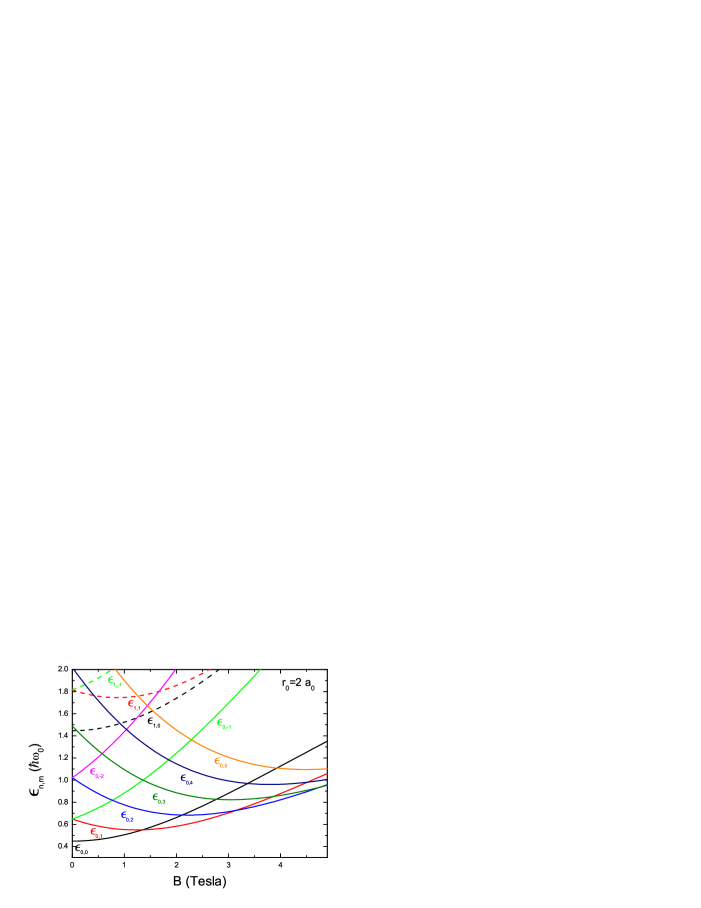
Figure 1: (Color online) Electron energy levels $\epsilon_{n,m}$ of a single quantum ring as a function of the magnetic field. The ring radius is fixed at $r_{0}=2a_{0}$.

$\begin{array}[]{cc}\includegraphics[angle={0},scale={.8}]{fig2a.eps}&\includegraphics[angle={0},scale={.8}]{fig2b.eps}\\ \includegraphics[angle={0},scale={.8}]{fig2c.eps}&\includegraphics[angle={0},scale={.8}]{fig2d.eps}\end{array}$

Figure 2: The phase diagram of the ground state of CQRs for a fixed ring radius ($r_{0}=2a_{0}$) for: (a) $N=$ 3, (b) $N=$ 4, (c) $N=$ 5, and (d) $N=$ 6. The insets indicate the three quantum numbers $(S_{z},M_{z},I_{z})$ which designate a ground state configuration.

The ground state (GS) energy of the coupled rings as a function of magnetic field is obtained from

$$E(N)=\sum_{jnm\sigma}\epsilon^{j}_{nm\sigma}-\frac{1}{2}\int d\mathbf{r}\rho(r)\left[V_{H}^{\rm{intra}}(r)+V_{H}^{\rm{inter}}(r)\right]$$

$$-\sum_{\sigma}\int d\mathbf{r}\rho^{\sigma}(r)V_{xc,\sigma}(r)-\frac{e}{c}\int d\mathbf{r}j_{p}(r)A_{xc}(r)$$

$$+2E_{xc}\left[\rho^{\uparrow}/2,\rho^{\downarrow}/2,\mathbf{\mathcal{V}}\right],$$ (5)

and the paramagnetic current density is given by

$$\mathbf{j}_{p}(r)=-\frac{\hbar}{m^{\ast}r}\mathbf{e}_{\theta}\sum_{\sigma}\sum_{n,m}^{N_{\sigma}}m|\phi_{nm\sigma}(r)|^{2}.$$ (6)

The measurable current density is equal to $\mathbf{j}(r)=\mathbf{j}_{p}(r)+(e/cm^{\ast})\rho(r)\mathbf{A}(r)$, where the second part corresponds to the diamagnetic current density.

In the $z$ direction we consider only the two lowest levels of the quantum wells that connect the two quantum rings. They are the symmetric bonding level and the antisymmetric antibonding level. The contribution from excited states due to confinement in the $z$ direction is neglected because the confinement in the $z$ direction is much stronger than that in the plane. Therefore the motion in the $z$ direction may be assumed to be decoupled from the in-plane motion and the Kohn-Sham equations can be solved separately from the Schrödinger equation in the $z$ direction that describes the tunneling between the quantum rings. In the limits of small and large inter-ring distance $d$, the results for single quantum rings are recovered. On the other hand, in the limit of small ring radius ($r_{0}\rightarrow 0$), results of the CQDs are recoveredbart , too.

III Ground state configurations

The energy levels $\epsilon_{n,m}$ of a single quantum ring with fixed radius $r_{0}=$2 $a_{0}$ ($r_{0}=$300 Å) are shown in Fig. 1 as a function of the magnetic field, where $a_{0}=\sqrt{\hbar/m^{*}\omega_{0}}$. The energy levels are labeled by the radial quantum number $n=0,1,2,...,$ and the angular quantum number $m=0,\pm 1,\pm 2,...$. The applied magnetic field breaks the $\pm m$ degeneracy and leads to angular momentum transitions in the ground state. Although we assume a fixed value for the ring radius $r_{0}=$2 $a_{0}$, the effects observed in Fig. 1 remains the same for different ring radius. The only difference is that the value of the magnetic field where the crossing occurs is rescaled and assumes a smaller value when the ring radius is increased. Using the single-particle picture one expects already that the few electron ground state of the CQRs will be strongly affected by the magnetic field. In contrast, qualitative different behavior from two vertically coupled quantum dots was found only when $N>8$ in the absence of the magnetic field lkc .

For the CQRs, the ground state configuration changes as a function of the inter-ring distance (tunneling energy) and magnetic field. The phase diagrams presented in Fig. 2 show the different configurations of the ground state of CQRs for a fixed ring radius $r_{0}$=2 $a_{0}$ and confinement energy $\hbar\omega_{0}=$5 meV as a function of the magnetic field and the inter-ring distance for (a) $N=$ 3, (b) $N=$ 4, (c) $N=$ 5 and (d) $N=$ 6. To perform the numerical calculation, we use typical GaAs values for the effective mass $m^{*}=0.067m_{0}$ and the dielectric constant $\epsilon_{s}=$12.4. For small magnetic field the GS configurations are the same as found previously for zero magnetic field lkc . With increasing magnetic field, many transitions in the ground state are observed, as can be seen in Figs. 2(a-d). The ground state phases are labeled by three quantum numbers $(S_{z},M_{z},I_{z})$: total spin $S_{z}$, total angular momentum $M_{z}$ and the isospin quantum number $I_{z}$, which is the difference between the number of electrons in the bonding state and in the antibonding state divided by 2.

For large inter-ring distance the two rings become decoupled. On the other hand, when the distance between them is small, they are strongly coupled acting as a single one with isospin number $I_{z}=N/2$ where all the electrons are situated in the bonding state. In the latter regime, six different ground state configurations with $I_{z}=3/2$ are found for $N$=3 ($B<4$ T) in Fig. 2(a). Qualitatively the different GS configurations as a function of the magnetic field can be understood through the single-particle (SP) picture in Fig. 1 together with Hund’s rules. For example, when $B<1.37$ T the SP energy level $\epsilon_{0,0}$ is lower than $\epsilon_{0,1}$, hence it can be filled with two electrons with opposite spin and the third electron occupies the state $\epsilon_{0,1}$ with spin up, resulting in the GS configuration $(1/2,1,3/2)$. But when $B>1.37$ T, the energy $\epsilon_{0,1}$ is lower than $\epsilon_{0,0}$ and it becomes energetically more favorable to fill the state $\epsilon_{0,1}$ with two electrons instead of $\epsilon_{0,0}$ and the transition $(1/2,1,3/2)\rightarrow(1/2,2,3/2)$ in the GS takes place. We also notice that in Fig. 2(a) this transition occurs effectively at lower magnetic field $B=0.85$ T because of the many-body effects. The other transitions $(1/2,2,3/2)\rightarrow(1/2,4,3/2)\rightarrow(1/2,5,3/2)\rightarrow(1/2,7,3/2)\rightarrow(1/2,8,3/2)$ are due to the same mechanism just explained. When the inter-ring distance increases, the difference between the bonding and antibonding states decreases and transitions in the GS configurations can be observed too. For large inter-ring distance in Fig. 2(a), the GS configurations with one electron in the antibonding state ($I_{z}=1/2$) are found. When the bonding-antibonding energy splitting $\Delta$ is less than the difference between two subsequent lateral bonding states the electron changes to the lowest unoccupied antibonding state yielding a GS transition. The state $(3/2,1,1/2)$ can not be explained only using the SP picture, because it has three aligned spins in different SP states. This is a clear manifestation of the many-body effects, where the total energy is minimized by the exchange interaction, when two electrons are in the same quantum state.

For $N$=4 in Fig. 2(b) we observe eight different GS configurations for $B<4$ T in the strong coupling regime ($I_{z}=2$) consistent with the SP picture and Hund’s rule. The total spin in the $z$ direction of these GS configurations alternates between 0 and 1 as a function of the external magnetic field. Increasing the inter-ring distance we found GS configurations with one ($I_{z}=1$) and two ($I_{z}=0$) electrons occupying the antibonding sates. Notice that for a fixed isospin $I_{z}=$1 or 2, the total angular momentum changes by $N/2=$2 as function of the magnetic field. This fact is related to the even number of electrons ($N=$4) occupying the CQRs. In the strong coupling regime, the even number of electrons can be arranged in such a way that $S_{z}$ oscillates between 0 and 1 and $M_{z}$ changes by $N/2$ with increasing the applied magnetic field. Also the state $(2,2,0)$ has all spins aligned due to the exchange interaction.

For $N$=5 seven different GS configurations in the strong coupling regime ($I_{z}=5/2$) are found in Fig. 2(c) for $B<4$ T. All of them are of total spin $S_{z}=1/2$. In this regime with increasing magnetic field, the total angular momentum alternately changes by 3 [$(1/2,1,5/2)\rightarrow(1/2,4,5/2)$] and by 2 [$(1/2,4,5/2)\rightarrow(1/2,6,5/2)$]. Since the number of electrons is $N=$5, two SP-levels are filled by two pair electrons and the third level by a single electron, which causes a change of the angular momentum by either 2 or 3 with increasing magnetic field. Increasing the inter-ring distance we found GS configurations with one ($I_{z}=3/2$) and two ($I_{z}=1/2$) electrons occupying the antibonding states. For these configurations the total spin can achieve values larger than 1/2. The states with total spin $S_{z}=3/2$ and isospin $I_{z}=3/2$ or $I_{z}=1/2$ are induced by the exchange interaction. Also the exchange interaction leads to the emergence of the maximum spin polarized state $(5/2,4,1/2)$. For intermediate $d$-values, we have $\Delta M_{z}$=1 transitions with increasing magnetic field corresponding to a single angular momentum increase of a single electron in this molecular state.

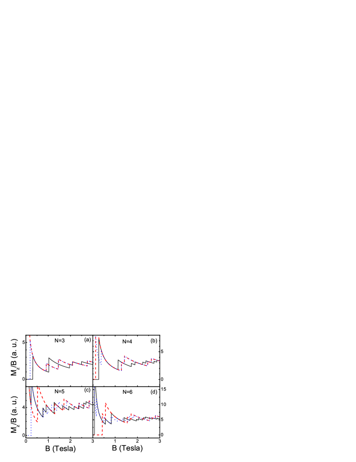
Figure 3: (Color online) $M_{z}/B$ as a function of magnetic field for different inter-ring separations $d=$30 Å (red dash curves), 50 Å (blue dotted curves), and 70 Å (black solid curves).

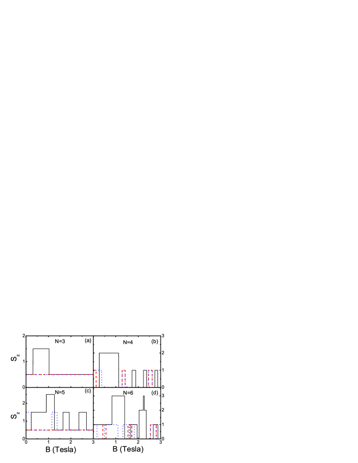
Figure 4: (Color online) The same as Fig. 3 but now for spin $S_{z}$.

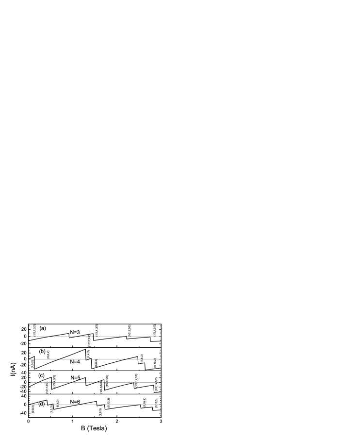
Figure 5: The persistent current as a function of the magnetic field in the strong coupling regime ($d=30$ Å) for CQRs with different number of electrons: (a) $N=3$, (b) $N=4$, (c) $N=5$, and (d) $N=6$.

For $N=6$ in Fig. 2(d) nine different GS configurations are found in the strong coupling regime ($I_{z}$=3) for $B<4$ T. Notice that for $I_{z}$=3 the total angular momentum changes by $N/2$=3 as function of the magnetic field due to the even number of electrons ($N$=6) in the CQRs. Increasing the inter-ring distance we found the GS configurations with one ($I_{z}=2$), two ($I_{z}=1$) and three ($I_{z}=0$) electrons occupying the antibonding states. When $I_{z}=2$, the total spin is $S_{z}=1$ because the bonding states are occupied by 5 electrons and the GS configurations are the same as found earlier for $N=5$ in the strong coupling regime, which always have one electron unpaired and the lowest antibonding state is filled with one more spin 1/2 electron. Many different states are induced by the exchange interaction when $N=6$, e.g.,, the eight states composed with total spin $S_{z}=1$ or $S_{z}=2$ and isospin $I_{z}=1$. The GS configurations $(3,6,0)$ and $(3,12,0)$ have all spins aligned.

In phase $(3,6,0)$, 3 electrons both in the bonding and the antibonding states occupy successive angular momentum states and the total angular momentum $M_{z}=\frac{N}{2}(\frac{N}{2}-1)$ which is the densest spin polarized electron configuration available in a quantum ring molecule of 6 electrons. Such a state is referred to as the maximum density droplet and was observed experimentally in a quantum dot in the presence of a magnetic field.mdd However, we notice that there is no corresponding single quantum ring phase for such a configuration. It exists only in the CQRs because of the many-body interactions combined with the inter-ring quantum tunneling effect. In fact, the phases (5/2,4,1/2) for $N=5$ found in Fig. 2(c), (2,2,0) for $N=4$ in Fig. 2(b), and (3/2,1,1/2) for $N=3$ in Fig. 2(a) are the maximum density droplet states in the QR molecules.

Figure 6: (Color online) The persistent current (solid curves) as a function of the magnetic field in the weak coupling regime ($d=70$ Å) for CQRs with different number of electrons: (a) $N=$ 3, (b) $N=$ 4, (c) $N=$ 5, and (d) $N=$ 6. The dashed (red) and dotted (blue) curves correspond to the bonding and anti-bonding currents, respectively.

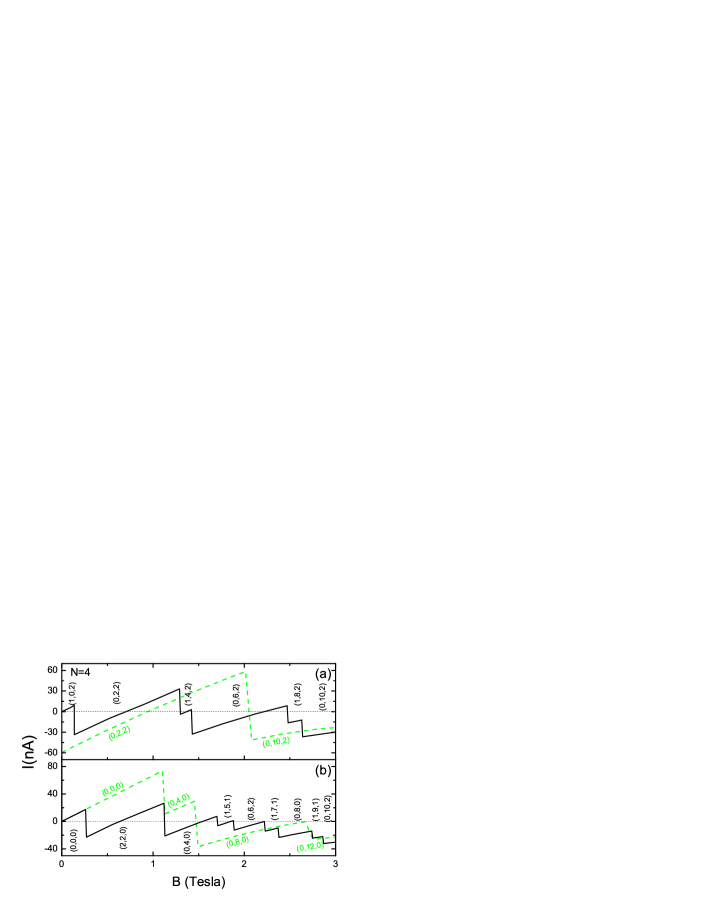
Figure 7: (Color online) The persistent current obtained through CSDFT calculation (solid black curve) and the single particle approximation (dashed green curve), considering the CQRs with four electrons in both (a) strong ($d=30$ Å) and (b) weak coupling regime ($d=70$ Å).

Figure 8: The total spin-current considering (a) $N=3$ in the strong coupling regime ($d=30$ Å) and (b) for $N=6$ in the weak coupling regime ($d=70$ Å).

In order to show more clearly the behavior of the total angular momentum and total spin in the CQRs, we plot $M_{z}/B$ and $S_{z}$ as a function of magnetic field in Fig. 3 and Fig. 4, respectively, for different inter-ring distances $d=$30 Å (the dash curves), 50 Å (the dotted curves), and 70 Å (the solid curves). The oscillation of $M_{z}/B$ in Fig. 3 is related to the magnetization of the CQRs and the corresponding persistent current which will be shown below. In Fig. 4 we see that with increasing the distance between the two rings the spin polarization of the system is enhanced. Generally, the QR molecule in the weak coupling regime ($d=$70 Å) is spin-polarized in a wider range of magnetic field than that in the strong coupling regime ($d=$30 Å, which is practically in the atomic regime). The maximum spin polarization $S_{z}=N/2$ always occurs in the molecular phases in the weak coupling regime at finite magnetic field.

IV Persistent current

In Fig. 5 the persistent current is shown, determined byemperador $I=\int j(r)dr$, as a function of the magnetic field in the strong coupling regime ($d=30$ Å) for different number of electrons $N=$ 3, 4, 5 and 6. The diamagnetic contribution to the persistent current in our model can be evaluated analytically and is given by $I_{d}=\frac{eNB}{4\pi m^{\ast}c}$. When the number of electrons in the CQRs is odd ($N$=3, 5), the persistent current oscillates with linear segments, and the different segments appear because of the change in the total angular momentum. As can be viewed in Figs. 3(a) and 3(c), for $d=30$ Å the total angular momentum changes as function of the magnetic field. The total momentum increases from $M_{z}^{<}$ to $M_{z}^{>}$ with increasing magnetic field following the rule $M_{z}^{>}=M_{z}^{<}+(N\pm 1)/2$ indicated in Fig. 2. These relations for the total angular momentum in the strong coupling regime can be explained by the breaking of the $\pm m$ degeneracy and the crossing between states with angular quantum number $(m+1)$ and $\pm m$. For example, in the case of $N=5$ and $B<0.8$ T the SP energy levels can be filled in the following way: two electrons in the state $\epsilon_{0,0}$, two in $\epsilon_{0,1}$ and one in $\epsilon_{0,-1}$, which gives the GS $(1/2,1,5/2)$. Increasing the magnetic field the state $\epsilon_{0,2}$ crosses the state $\epsilon_{0,-1}$ at $B=0.8$ T and now the configuration of the GS is $(1/2,4,5/2)$ with: two electrons in the state $\epsilon_{0,0}$, two in $\epsilon_{0,1}$ and one in $\epsilon_{0,2}$. For $B>1.37$ T the level $\epsilon_{0,2}$ crosses the $\epsilon_{0,1}$ and the configurations of the GS is $(1/2,6,5/2)$ with: one electron in the state $\epsilon_{0,0}$, two in $\epsilon_{0,1}$ and two in $\epsilon_{0,2}$. Therefore the total angular momentum jumps from $M_{z}=1$ to $M_{z}=4$ and from $M_{z}=4$ to $M_{z}=6$ respecting the crossing between the SP energy levels. However, the value of the magnetic field at which the GS transition occurs is not exactly the same as the SP crossings because it is reduced by the electron-electron interaction.

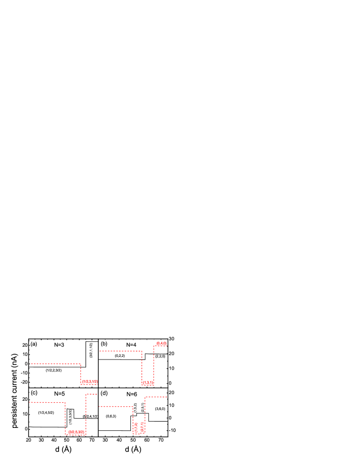
Figure 9: (Color online) The persistent current for CQRs with: (a) $N=$ 3, (b) $N=$ 4, (c) $N=$ 5, and (d) $N=$ 6, as a function of the distance between the two coupled quantum rings. Also, we consider two different values of magnetic field $B=1$ T (black solid curve) and $B=1.1$ T ($B=1.25$ T) (red dashed curve) in the upper (bottom) panel.

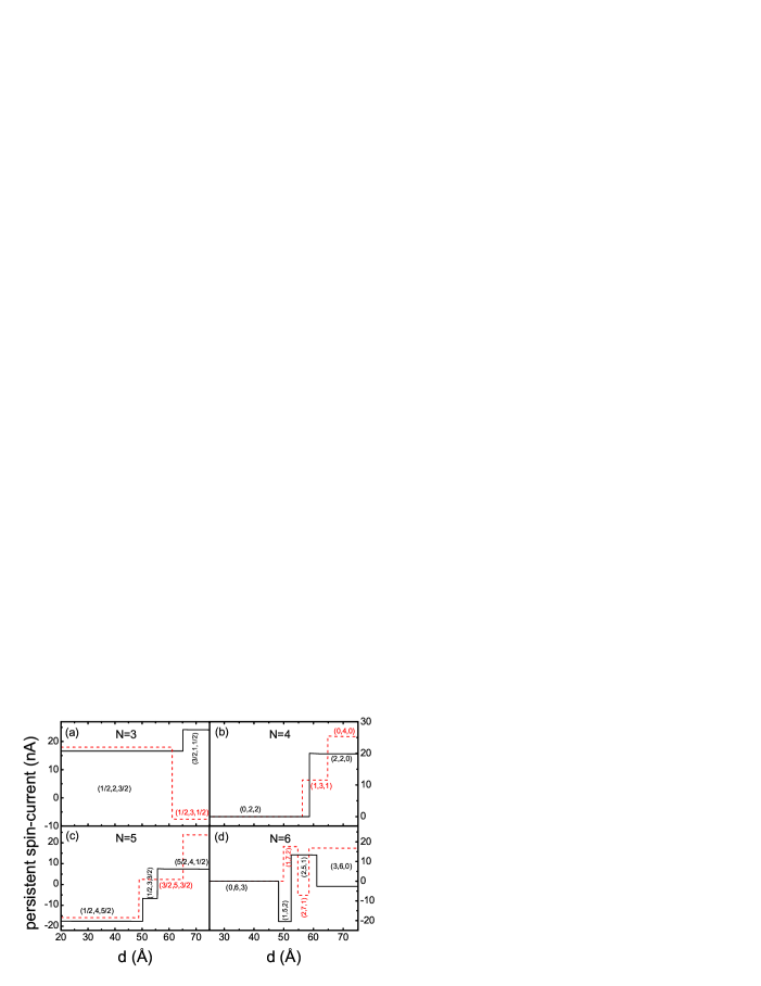
Figure 10: (Color online) The persistent spin-current for CQRs with: (a) $N=$ 3, (b) $N=$ 4, (c) $N=$ 5, and (d) $N=$ 6, as a function of the distance between the two coupled quantum rings. Also, we consider two different values of magnetic field $B=1$ T (black solid curve) and $B=1.1$ T ($B=1.25$ T) (red dashed curve) in the upper (bottom) panel.

When the number of electrons is even $N=4$ [see Fig. 5(b)] or $N=6$ [see Fig. 5(d)] in the strong coupling regime ($d=30$ Å), the persistent current also oscillates with linear segments, but an additional fine structure is found. In this case, the difference between two consecutive total angular momentum transitions as a function of the magnetic field is always equal to $M_{z}^{>}-M_{z}^{<}=N/2$ as shown in Figs. 5(b) and 5(d). When the total spin is different from zero ($S_{z}\neq 0$), the ground state is unstable because it corresponds to an open-shell system, and consequently an intermediate structure in the total persistent current appears. For $N$-even, $S_{z}$ oscillates between 0 and 1 [see the dash curves in Figs. 4(b) and 4(d)] and these transitions are reflected in the total persistent current. The more stable linear segments correspond to closed-shell configurations ($S_{z}=0$).

The persistent current as a function of the magnetic field in the weak coupling regime ($d=70$ Å) for different number of electrons $N=$ 3, 4, 5 and 6 are shown in Figs. 6(a-d), respectively. The dotted and dashed curves correspond to the bonding and antibonding currents, respectively. The bonding (antibonding) current is the contribution of the electrons in the bonding (antibonding) state to the persistent current. For example, the bonding paramagnetic current density is found by considering only the contribution of the bonding states in Eq. (6), and so on. The solid curve represents the total current, which is the sum of the bonding and antibonding currents. In the weak coupling regime, the bonding and antibonding states can be occupied simultaneously as can be viewed through the changes in $I_{z}$ indicated in Figs. 2(a-d). Therefore, different combinations of the total angular momentum are possible as a function of the magnetic field and any change of $M_{z}$ leads to a jump in the persistent current. For large values of the magnetic field, such jumps become more frequent because of a rapid variation of the angular momentum at large magnetic fields and consequently the amplitude of the oscillation in the the persistent current is reduced.

In order to understand the relevance of the many-body effects, we show in Fig. 7 the persistent current calculated using CSDFT (solid curve) and using the single particle approximation (dashed curve), considering the CQRs with four electrons in both the strong [see Fig. 7(a)] and the weak [see Fig. 7(b)] coupling regime. When the single-particle approximation is considered, we note that most of the little jumps in the persistent current are missing and in some regions the single-particle results give an opposite persistent current compared to the persistent current evaluated by CSDFT. Therefore, through this comparison in Fig. 7 we clearly see the importance of the many-body interactions when estimating the persistent currents in CQRs.

We present in Fig. 8 the persistent spin-current for a CQRs with (a) $N=3$ in the strong coupling regime ($d=30$ Å) and (b) $N=6$ in the weak coupling regime ($d=70$ Å). The spin-current is defined as the difference between the current of electrons with spin-up and with spin-down. The paramagnetic spin-current density is given explicitly by $\mathbf{j}^{s}_{p}(r)=-\frac{\hbar}{m^{\ast}r}\mathbf{e}_{\theta}\left(\sum_{n,m}^{N_{\uparrow}}m|\phi_{nm\uparrow}(r)|^{2}-\sum_{n,m}^{N_{\downarrow}}m|\phi_{nm\downarrow}(r)|^{2}\right)$. The diamagnetic contribution for the persistent spin-current is given by $I^{s}_{d}=\frac{eB(N^{\uparrow}-N^{\downarrow})}{4\pi m^{\ast}c}$. The persistent spin-current is zero in the magnetic field ranges where the total spin $S_{z}$ in a certain GS configuration is zero as can be viewed in Fig. 8(b). When the CQRs is occupied by an odd number of electrons, the persistent spin-current is never zero [see Fig. 8(a)] because now always a not-aligned electron is present.

In addition to the external magnetic field, the distance between the two quantum rings is another important parameter affecting the persistent current and the spin-current. Fig. 9(a) shows the persistent current for a CQRs with $N=3$ for different values of the magnetic field (a) $B=1$ T (solid curve) and $B=1.1$ T (dashed curve). The respective spin-currents are presented in Fig. 10(a). For the CQRs with $N=4$ we plot the same quantities in Fig. 9(b) and Fig. 10(b) for the magnetic fields $B=1$ T (solid curves) and $B=1.1$ T (dashed curves). We plot the persistent current (spin-current) in Fig. 9(c) (Fig. 10(c)) for a CQRs with $N=5$ for the magnetic fields B=1 T (the solid curves) and for $B=1.25$ T (the dashed curves). The persistent current in Fig. 9(d) and persistent spin-current in Fig. 10(d) are evaluated for different values of the magnetic field B=1 T (solid curves) and $B=1.25$ T (dashed curves) for a CQRs with $N=6$. In Figs. 9-10 we notice that for a fixed value of the magnetic field, the persistent current (spin-current) as a function of the inter-ring distance is practically constant and exhibits a jump when a ground state transition occurs. Therefore, by varying the inter-ring distance for fixed value of the applied magnetic field, the GS configuration of the CQRs can be determined. For $N=3$ and $B=1$ T ($B=1.1$ T), we have the transition $(1/2,2,3/2)\rightarrow(3/2,1,1/2)$ ($(1/2,2,3/2)\rightarrow(1/2,3,1/2)$) as a function of the inter-ring distance. When $B=1$ T the total spin changes from $S_{z}=1/2$ to $S_{z}=3/2$ and the total angular momentum from $M_{z}=2$ to $M_{z}=1$. Therefore the total angular momentum decreases and the persistent current increases [see Fig. 9(a)], because of the reduction in the paramagnetic current [see Eq. (6)]. The increase in the total spin in the $z$-direction causes an amplification of the persistent spin-current, as can be viewed in Fig. 10(a). On the other hand, when $B=1.1$ T the total spin does not change and the total angular momentum decreases, which leads to a reduction of both the persistent current and the spin-current.

When the CQRs are filled with 4 electrons and the applied magnetic field is $B=1$ T, the transition $(0,2,2)\rightarrow(2,2,0)$ occurs as a function of the inter-ring distance. Increasing the magnetic field slightly ($B=1.1$ T), an intermediate GS configuration appears and now we have the transitions $(0,2,2)\rightarrow(1,3,1)\rightarrow(0,4,0)$. When $B=1$ T, the total spin changes from $S_{z}=0$ to $S_{z}=2$ and the total angular momentum is not affected. Thus the persistent current is almost unaltered [see Fig. 9(b)] and the persistent spin-current changes abruptly [see Fig. 10(b)], because all the carriers are spin polarized for $S_{z}=2$. Moreover, when $B=1.1$ T the persistent current firstly decreases (56Å$<d<$65Å) and afterwards increases ($d>$65Å) due to the increase of the angular momentum. The persistent spin-current is zero for $d<$56Å, because the net spin is zero in this range. For 56Å$<d<$65Å the persistent spin-current is different from zero and increases more for $d>$65Å, because of full alignment of the electron spins. For $N=5$, we choose two different magnetic fields $B=1$ T and $B=1.25$ T which gives the following GS transitions $(1/2,4,5/2)\rightarrow(1/2,3,3/2)\rightarrow(5/2,4,1/2)$ and $(1/2,4,5/2)\rightarrow(3/2,5,3/2)\rightarrow(5/2,4,1/2)$, respectively. The initial and final GS configurations are the same for these two magnetic fields and both have the same total angular momentum $M_{z}=4$, and only the GS configurations with $I_{z}=3/2$ are different. This difference brings an opposite behavior of the persistent current [see Fig. 9(c)] for the $I_{z}=3/2$ GS configurations and in one case (B=1 T) it increases and the other ($B=1.25$ T) decreases, due to the difference of total angular momentum in both cases. The latter-type behavior of the persistent spin-current [see Fig. 10(c)] in both cases ($B=1$ T and $B=1.25$ T) is a consequence of the increase in the spin polarization as a function of the inter-ring distance. The ground state transitions for the applied magnetic field $B=1$ T and $B=1.25$ T are respectively $(0,6,3)\rightarrow(1,5,2)\rightarrow(2,5,1)\rightarrow(3,6,0)$ and $(0,6,3)\rightarrow(1,7,2)\rightarrow(2,7,1)\rightarrow(3,6,0)$, when the CQRs are occupied with $N=6$ electrons. Again the initial and final GS configurations for the magnetic fields chosen are the same and in this case two intermediate configurations appear. When $B=1$ T ($B=1.25$ T), the persistent current [see Fig. 9(d)] increases (decreases) when the inter-ring distance corresponds to one of the intermediate configurations, because of the increase (decrease) in angular momentum. The persistent spin-current is zero for the GS configuration $(0,6,3)$ due to the spin-unpolarized electrons [see Fig. 10(d)]. The persistent spin-current [see Fig. 10(d)] of the intermediate GS configurations $(1,5,2)$ and $(2,7,1)$ ($(1,7,2)$ and $(2,5,1)$) decreases (increases) because the paramagnetic spin-current is larger (smaller) than the diamagnetic spin-current. The GS-configuration $(3,6,0)$ for $B=1$ T has a small spin-current due to the compensation of the paramagnetic spin-current by the diamagnetic spin-current, what does not happen for $B=1.25$ T, where the diamagnetic spin-current is larger than the paramagnetic spin-current.

V Summary

We studied systematically the electronic structure and the persistent current in two vertically coupled quantum rings as a function of an applied external magnetic field and the inter-ring distance. A rich variety of ground state configurations were found, that are induced by changing the inter-ring distance and the applied magnetic field. We found that these transitions are governed by some rules, which are related to the even/odd number of electrons, the single-particle picture, Hund’s rules and many-body effects. The found ground state configurations are summarized in phase diagrams, which generalize the previous B=0 resultslkc to non-zero values of the magnetic field. Moreover, the persistent current and spin-current were evaluated for the CQRs and we showed that their variation with magnetic field is governed by the values of the total angular momentum and total spin. Therefore, once the GS configuration is known the persistent current and spin-current can be estimated. Furthermore, we provide useful information to determine the ground state configuration through measurements of the persistent current. Also we showed that the electron-electron interaction strongly influences the sign and size of the persistent current.

The simple rules and the complete set of results for $N$=3,4,5, and 6 electrons shown in the present work may not be compared to available experimental data. The reason for that is because we assumed a system composed of two symmetric QRs vertically coupled containing few electrons and until now the experimental fabrication of such an arrangement is quite difficult. Nonetheless, we believe that our results and conclusions may be very useful to interpret experimental data when those difficulties are overcome.

- (1) A. I. Ekimov, A. L. Efros, and A. A. Onushchenko, Solid State Commun. 56, 921 (1985).
- (2) Quantum Dots, L. Jacak, P. Hawrylak, and A. Wojs, (Springer, Berlin, 1998); Quantum Dots, T. Chakraborty, (Elsevier, Amsterdam, 1999); Quantum Dot Heterostructures D. Bimberg, M. Grundmann and N. N. Ledentsov (Wiley, London, 2001); Electron Transport in Quantum Dots J. P. Bird (Kluwer Academic Publishers, Boston, 2003).
- (3) R. Held, S. Lüscher, T. Heinzel, K. Ensslin, and W. Wegscheider, Appl. Phys. Lett. 75, 1134 (1999); A. Fuhrer, S. Lüscher, T. Ihn, T. Heinzel, K. Ensslin, W. Wegscheider, and M. Bichler, Nature (London) 413, 822 (2001).
- (4) Z. Gong, Z. C. Niu, S. S. Huang, Z. D. Fang, B. Q. Sun, and J. B. Xia, Appl. Phys. Lett. 87, 093116 (2005).
- (5) J. M. García, G. Medeiros-Ribeiro, K. Schmidt, T. Ngo, J. L. Feng, A. Lorke, J. Kotthaus, and P. M. Petroff, Appl. Phys. Lett. 71, 2014 (1997); A. Lorke, R. J. Luyken, A. O. Govorov, J. P. Kotthaus, J. M. García, and P. M. Petroff, Phys. Rev. Lett. 84, 2223 (2000).
- (6) Aharonov-Bohm and other cyclic phenomena, J. Hamilton (Springer-Verlag, Berlin, 1997).
- (7) L. K. Castelano, G.-Q. Hai, B. Partoens, and F. M. Peeters, Phys. Rev. B 74, 045313 (2006); Braz. J. Phys. 36, 936 (2006); Phys. Status Solidi C 4, 560 (2007).
- (8) F. Malet, M. Barranco, E. Lipparini, R. Mayol, M. Pi, J. I. Climente, and J. Planelles, Phys. Rev. B 73, 245324 (2006).
- (9) Y. Saiga, D. S. Hirashima, and J. Usukura, Phys. Rev. B 75, 045343 (2007).
- (10) B. Szafran, S. Bednarek, and M. Dudziak, Phys. Rev. B 75, 235323 (2007).
- (11) B. Szafran, Phys. Rev. B 77, 235314 (2008); Phys. Rev. B 77, 205313 (2008).
- (12) T. Chwiej and B. Szafran, Phys. Rev. B 78, 245306 (2008).
- (13) M. Royo, F. Malet, M. Barranco, M. Pi, and J. Planelles, Phys. Rev. B 78, 165308 (2008).
- (14) Y. Z. He and C. G. Bao, Eur. Phys. J. B 62, 465 470 (2008).
- (15) G. Piacente and G.-Q. Hai, J Appl. Phys. 101, 124308 (2007).
- (16) L. G. G. V. Dias da Silva, J. M. Villas-Bôas, and S. E. Ulloa, Phys. Rev. B 76, 155306 (2007).
- (17) F. Suárez, D. Granados, M. L. Dotor, and J. M. García, Nanotechnology 15, S126 (2004).
- (18) D. Granados, J. M. García, T. Ben, and S. I. Molina, Appl. Phys. Lett. 86, 071918 (2005).
- (19) T. Mano, T. Kuroda, S. Sanguinetti, T. Ochiai, T. Tateno, J. Kim, T. Noda, M. Kawabe, K. Sakoda, G. Kido, and N. Koguchi, Nano Lett. 5, 425 (2005).
- (20) T. Kuroda, T. Mano, T. Ochiai, S. Sanguinetti, K. Sakoda, G. Kido, and N. Koguchi, Phys. Rev. B 72, 205301 (2005).
- (21) N. A. J. M. Kleemans, I. M. A. Bominaar-Silkens, V. M. Fomin, V. N. Gladilin, D. Granados, A. G. Taboada, J. M. García, P. Offermans, U. Zeitler, P. C. M. Christianen, J. C. Maan, J. T. Devreese, and P. M. Koenraad, Phys. Rev. Lett. 99, 146808 (2007).
- (22) L. K. Castelano, G.-Q. Hai, B. Partoens, and F. M. Peeters, Phys. Rev. B 78, 195315 (2008).
- (23) J. C. Lin and G. Y. Guo, Phys. Rev. B 65, 035304 (2001).
- (24) S. Viefers, P. S. Deo, S. M. Reimann, M. Manninen, and M. Koskinen, Phys. Rev. B 62, 10668 (2000).
- (25) G. Vignale and M. Rasolt, Phys. Rev. Lett. 59, 2360 (1987); Phys. Rev. B 37, 10685 (1988).
- (26) B. Partoens and F. M. Peeters, Europhys. Lett. 56, 86 (2001).
- (27) D. Levesque, J. J. Weis and A. H. MacDonald, Phys. Rev. B 30, 1056 (1984).
- (28) B. Tanatar and D. M. Ceperley, Phys. Rev. B 39, 5005 (1989).
- (29) T. H. Oosterkamp et al., Phys. Rev. Lett. 82, 2931 (1999); A. MacDonald et al., Aust. J. Phys. 46, 345 (1993).
- (30) A. Emperador, M. Pi, M. Barranco and E. Lipparini, Phys. Rev. B 64, 155304 (2001).