Pion form factor in QCD sum rules, local duality approach, and O$(\mathcal{A}_{2})$ fractional analytic perturbation theory

Abstract

Using the results on the electromagnetic pion Form Factor (FF) obtained in the $O(\alpha_{s})$ QCD sum rules with non-local condensates [1] we determine the effective continuum threshold for the local duality approach. Then we apply it to construct the $O(\alpha_{s}^{2})$ estimation of the pion FF in the framework of the fractional analytic perturbation theory.

In this paper we use the results on the electromagnetic pion FF $F_{\pi}(Q^{2})$ in the spacelike region $Q^{2}=1-10$ GeV², obtained in the $O(\alpha_{s})$ QCD Sum Rule (SR) approach with nonlocal condensates (NLC) [1], in order to estimate the next-to-next-to-leading (or the $O(\alpha_{s}^{2})$) order (NNLO) correction to the pion FF using both the Fractional Analytic Perturbation Theory (FAPT) and the Local Duality (LD) approach. First, we describe the LD approximation in the pion FF calculation and discuss how it is possible to obtain the main ingredient of this approach, namely, the continuum threshold $s_{0}(Q^{2})$ as a function of $Q^{2}$. Then we explain why one need to use FAPT in estimating the NNLO result for the factorized part of the pion FF. Next, we describe our model [2] for matching function, gluing soft and hard parts to the complete pion FF. After that we show how to apply FAPT to estimate the NNLO pion FF using improved model for matching function.

1 Pion FF in the Local Duality approach

The LD SR [3, 4] is produced from the original QCD SR in the $M^{2}\rightarrow\infty$ limit. For this reason it has no condensate contributions. The main nonperturbative ingredient in this approach is the effective continuum threshold $s_{0}^{\text{LD}}$ — it inherits all the nonperturbative information from the original QCD SR. At the $(l+1)$-loop order we have

$$F_{\pi}^{\text{LD};(l)}(Q^{2},S)\equiv\int\limits_{0}^{S}\!\!\!\int\limits_{0}^{S}\!\!\rho_{3}^{(l)}(s_{1},s_{2},Q^{2})\,\frac{ds_{1}\,ds_{2}}{f_{\pi}^{2}}\,,$$ (1)

where $S$ should be substituted by the LD effective threshold, $s_{0}^{\text{LD};(l)}(Q^{2})$, and $\rho_{3}^{(l)}(s_{1},s_{2},Q^{2})$ is the three-point $(l+1)$-loop spectral density. In the leading order the integration can be done analytically: $F_{\pi}^{\text{LD};(0)}(Q^{2},S)=[S/(4\pi^{2}f_{\pi}^{2})]\,[1-(Q^{2}+6S)/(Q^{2}+4S)\,\sqrt{Q^{2}/(Q^{2}+4S)}]$. The LD prescription for the corresponding correlator [5, 4] implies the relations

$$s_{0}^{\text{LD};(0)}(0)=4\,\pi^{2}\,f_{\pi}^{2}\simeq 0.7~{}\text{GeV}^{2}$$ (2a)

and

$$s_{0}^{\text{LD};(1)}(0)=\frac{4\,\pi^{2}\,f_{\pi}^{2}}{1+\alpha_{s}(Q_{0}^{2})/\pi}\simeq 0.6~{}\text{GeV}^{2}\,,~{}~{}~{}$$ (2b)

where $Q_{0}^{2}$ is of the order of $s_{0}^{\text{LD};(0)}(0)$. This prescription is a strict consequence of the Ward identity for the AAV correlator due to the vector-current conservation. In principle, the $Q^{2}$ dependence of the LD parameter $s_{0}^{\text{LD}}(Q^{2})$ (1) should be determined from the QCD SR at $Q^{2}\gtrsim 1$ GeV². But as explained in [1] the standard QCD SR becomes unstable at $Q^{2}>3$ GeV² because of the appearance of terms in the condensate contributions linearly growing with $Q^{2}$ [6, 7]. For this reason, this dependence was known only for $Q^{2}\leq 3$ GeV² and, therefore, most authors usually used the constant approximation $s_{0}^{\text{LD};(0)}(Q^{2})\simeq s_{0}^{\text{LD};(0)}(0)$, like in [3, 8, 2, 9], or a slightly $Q^{2}$-dependent approximation $s_{0}^{\text{LD};(1)}(Q^{2})\simeq 4\,\pi^{2}\,f_{\pi}^{2}/(1+\alpha_{s}(Q^{2})/\pi)$, like in [10].

But now, due to the knowledge of the NLC QCD SR prediction [1] for the pion FF for $Q^{2}=1-10$ GeV², we can estimate the effective LD threshold $s_{0}^{\text{LD}}(Q^{2})$ which reproduce these predictions in the LD approach. Results are shown in Fig. 1. It can be represented in this $Q^{2}$ range by the following interpolation formula:

$$s_{0}^{\text{LD}}(Q^{2})=0.57+0.461\,\tanh\left[\frac{0.0954\,Q^{2}}{\text{GeV}^{2}}\right]\,.$$ (3)

We see that $s_{0}^{\text{LD}}(Q^{2})$ in the mentioned range of $Q^{2}$ is monotonically increasing function. Therefore $s_{0}^{\text{LD}}(Q^{2})\neq s_{0}^{\text{SR}}(Q^{2})\approx 0.7$ GeV² and due to this difference the LD approaches of [2, 9, 10] produces significantly lower predictions for $Q^{2}\,F_{\pi}(Q^{2})$ as compared with QCD SRs with NLC.

Figure 1: The effective LD threshold $s_{0}^{\text{LD}}$ as a function of $Q^{2}$.

2 Using FAPT for NNLO estimation

In order to estimate the NNLO contribution to the pion FF in the QCD SR approach one needs to know the three-loop spectral density $\rho_{3}^{(3)}(s_{1},s_{2},Q^{2})$ and this is a complicated task. We want to avoid this tricky calculation and suggest to use the known collinear two-loop result, the LD model for the soft part with improved $s_{0}^{\text{LD}}(Q^{2})$, and matching procedure of [2]. And one needs to use (F)APT for the two-loop collinear expression, as been shown in [2, 11], in order to have practical independence with respect to renormalization and factorization scale setting.

To ‘glue’ together the LD model for the soft part, $F_{\pi}^{\text{LD},(0)}(Q^{2})$ (which is dominant at small $Q^{2}\leq 1$ GeV²), with the perturbative hard-rescattering part, $F_{\pi}^{\text{pQCD},(2)}(Q^{2})$ (which provides the leading perturbative $O(\alpha_{s})+O(\alpha_{s}^{2})$ corrections and is dominant at large $Q^{2}\gg 1$ GeV²), in such a way as to ensure the validity of the Ward identity (WI) $F_{\pi}^{\text{WI};(2)}(0)=1$, we apply the matching procedure, introduced in [2]:

$$F_{\pi}^{\text{WI};(2)}(Q^{2})=F_{\pi}^{\text{LD},(0)}(Q^{2})~{}~{}~{}~{}~{}~{}~{}~{}~{}~{}~{}~{}~{}~{}~{}~{}~{}~{}~{}~{}~{}~{}$$

$$~{}~{}~{}+\left(\frac{Q^{2}}{2s_{0}^{(2)}+Q^{2}}\right)^{2}F_{\pi}^{\text{pQCD},(2)}(Q^{2})$$ (4)

with $s_{0}^{(2)}\simeq 0.6$ GeV². In order to test the quality of the matching prescription given by Eq. (4), we propose to compare it with the LD model (1) evaluated at the one-loop order (i.e., in the $O(\alpha_{s})$-approximation [9, 10]). To this end, we construct the analogous $O(\alpha_{s})$-model $F_{\pi}^{\text{WI};(1)}(Q^{2})$, where we substitute $F_{\pi}^{\text{pQCD},(2)}(Q^{2})$ by $F_{\pi}^{\text{pQCD},(1)}(Q^{2})=2\,\alpha_{s}(Q^{2})\,s_{0}^{\text{LD};(0)}(0)/\pi\,Q^{2}$ and imply the same prescription for the effective LD threshold as in [10], i. e. (2b). It is worth to note that the model $F_{\pi}^{\text{WI};(1)}(Q^{2})$, suggested in [2], works quite well, although it was proposed without the knowledge of the exact two-loop spectral density, which became available later [9]. The key feature of this matching recipe is that it uses information on $F_{\pi}(Q^{2})$ in two asymptotic regions:

1. $Q^{2}\to 0$, where the Ward identity dictates $F_{\pi}(0)=1$ and hence $F_{\pi}(Q^{2})\simeq F_{\pi}^{\text{LD},(0)}(Q^{2})$,

2. $Q^{2}\to\infty$, where $F_{\pi}(Q^{2})\simeq F_{\pi}^{\text{pQCD},(1)}(Q^{2})$

in order to join properly the hard tail of the pion FF with its soft part. Numerical analysis shows that the applied prescription yields a pretty accurate result, with a relative error varying in the range 5% at $Q^{2}=1$ GeV² to 9% at $Q^{2}=3-30$ GeV².

Now, when the spectral density $\rho_{3}^{(1)}(s_{1},s_{2},Q^{2})$ is known [9], it is possible to improve the representation of the LD part by taking into account the leading $O(\alpha_{s})$ correction in the electromagnetic vertex. We suggest the following improved WI model

$$F_{\pi;\text{imp}}^{\text{WI};(1)}(Q^{2},S)=F_{\pi}^{\text{LD};(0)}(Q^{2},S)~{}~{}~{}~{}~{}~{}~{}~{}~{}~{}~{}~{}~{}~{}~{}$$

$$~{}~{}~{}+\frac{S}{4\pi^{2}f_{\pi}^{2}}\,\frac{\alpha_{s}(Q^{2})}{\pi}\,\left(\frac{2S}{2S+Q^{2}}\right)^{2}$$

$$+\frac{S}{4\pi^{2}f_{\pi}^{2}}\,F^{\text{pQCD},(1)}_{\pi}(Q^{2})\,\left(\frac{Q^{2}}{2S+Q^{2}}\right)^{2}$$ (5)

with subsequent substitution $S\to s_{0}^{\text{LD};(1)}(Q^{2})$. We explicitly display the dependence on the threshold $S$ in Eq. (5)—the aim being to apply it later on with $S=s_{0}^{\text{LD}}(Q^{2})$, the latter value being extracted by comparing the NLC QCD SR results with the LD approximation. Numerical evaluation of this new WI model in comparison with the exact LD result in the one-loop approximation shows that the quality of the matching condition is improved: the relative error is reduced, reaching 4% at $Q^{2}=1-10$ GeV².

Proceeding along similar lines of reasoning, we construct the two-loop WI model $F_{\pi}^{\text{WI};(2)}(Q^{2},s_{0}^{\text{LD};(2)}(Q^{2}))$ for the pion FF to obtain

$$F_{\pi}^{\text{WI};(2)}(Q^{2},S)=F_{\pi}^{\text{LD};(0)}(Q^{2},S)~{}~{}~{}~{}~{}~{}~{}~{}~{}~{}~{}~{}~{}~{}~{}$$

$$~{}~{}~{}+\frac{S}{4\pi^{2}f_{\pi}^{2}}\,\frac{\alpha_{s}(Q^{2})}{\pi}\,\left(\frac{2S}{2S+Q^{2}}\right)^{2}$$

$$+\frac{S}{4\pi^{2}f_{\pi}^{2}}\,F^{\text{FAPT},(2)}_{\pi}(Q^{2})\,\left(\frac{Q^{2}}{2S+Q^{2}}\right)^{2},$$ (6)

where $F^{\text{FAPT},(2)}_{\pi}(Q^{2})$ is the analyticized expression generated from $F^{\text{pQCD},(2)}_{\pi}(Q^{2})$ using FAPT (see Refs. [12, 13, 11]) to get a result which appears to be very close to the outcome of the default scale setting ($\mu_{\text{R}}^{2}=\mu_{\text{F}}^{2}=Q^{2}$), investigated in detail in [2] in the APT approach. FAPT is needed here in order to obtain analytic expressions for the pion FF in both possible cases of factorization scale setting:

1. For $\mu_{\text{F}}^{2}=Q^{2}$ there appear factors of the type $\left[\alpha_{s}(Q^{2})\right]^{\nu}$ with fractional powers $\nu=\gamma_{n}/(2\,b_{0})$ due to the pion distribution amplitude evolution;

2. For $\mu_{\text{F}}^{2}=\textsl{const}$ there appears factor $\left[\alpha_{s}(Q^{2})\right]^{2}\ln(Q^{2}/\mu_{\text{F}}^{2})$.

In any case, the NNLO correction involves the analytic image of the second power of the coupling, $\mathcal{A}_{2}(Q^{2})$. For this reason we name the whole $F^{\text{FAPT},(2)}_{\pi}(Q^{2})$ term as $O(\mathcal{A}_{2})$ contribution.

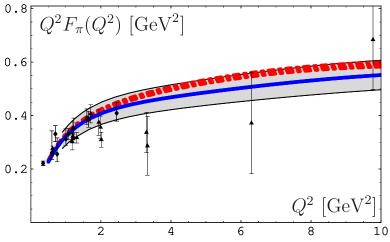
Figure 2: We show as a narrow dash-dotted strip the predictions for the pion FF, obtained in the two-loop WI model, Eq. (6), using the improved Gaussian model. The width of the strip is due to the variation of the Gegenbauer coefficients $a_{2}$ and $a_{4}$ (needed to calculate the collinear part $F_{\pi}^{\text{pQCD},(2)}(Q^{2})$) in the corresponding shaded bands for the pion DA (indicated by the central solid line). Note that this dash-dotted strip shows the effect of $O(\mathcal{A}_{2})$ correction only for the central solid curve of the shaded band.

Interesting to note here, that in the case of the one-loop approximation the relative error of WI model (5) appears to be of the order of 10%. The relative $O(\alpha_{s}^{2})$-contribution to the pion FF is of the order of 10%, as has been shown in [2, 11]. Hence, the relative error of our estimate is of the order of 1%—provided we take into account the $O(\alpha_{s})$-correction exactly via the specific choice of $s_{0}(Q^{2})$, as done in (3).

The results obtained for the pion FF with our two-loop model, i.e., Eq. (6), and using the effective LD thresholds $s_{0}^{\text{LD}}(Q^{2})$, are displayed in Fig. 2. We see from this figure that the main effect of the NNLO correction peaks at $Q^{2}\gtrsim 4$ GeV², reaching the level of $3-10$%.

Conclusions

• We showed here that the local duality model for pion FF suffers from the threshold $s_{0}(Q^{2})$ uncertainty. We fixed this uncertainty by demanding that the LD model with right setting for $s_{0}(Q^{2})$ should reproduce results for pion FF obtained in the Borel SRs with NLC [1]. Our results show that $s_{0}^{\textbf{LD}}(Q^{2})$ grows with $Q^{2}$.

• Our rough model for matching function in [2] appears to be of good quality ($\approx 10\%$) and we managed to improve it here to have quality of $\approx 5\%$.

• Using FAPT and improved matching function we estimated NNLO correction to the pion FF to be of the order of $\approx 3-10\%$.

• Our strip of predictions for the pion FF is in a good agreement with existing experimental data of Cornell [14] and JLab [15].

References

• [1] A.Β P. Bakulev, A.Β V. Pimikov, and N.Β G. Stefanis, Phys. Rev. D79 (2009) 093010.
• [2] A.Β P. Bakulev, K. Passek-Kumerički, W. Schroers, and N.Β G. Stefanis, Phys. Rev. D70 (2004) 033014, 079906(E).
• [3] V.Β A. Nesterenko and A.Β V. Radyushkin, Phys. Lett. B115 (1982) 410.
• [4] A.Β V. Radyushkin, Acta Phys. Polon. B26 (1995) 2067.
• [5] M.Β A. Shifman, A.Β I. Vainshtein, and V.Β I. Zakharov, Nucl. Phys. B147 (1979) 385; ibid. 448; ibid. 519.
• [6] B.Β L. Ioffe and A.Β V. Smilga, Nucl. Phys. B216 (1983) 373.
• [7] V.Β A. Nesterenko and A.Β V. Radyushkin, JETP Lett. 39 (1984) 707.
• [8] A.Β P. Bakulev, A.Β V. Radyushkin, and N.Β G. Stefanis, Phys. Rev. D62 (2000) 113001.
• [9] V.Β V. Braguta and A.Β I. Onishchenko, Phys. Lett. B591 (2004) 267.
• [10] Victor Braguta, Wolfgang Lucha, and Dmitri Melikhov, Phys. Lett. B661 (2008) 354.
• [11] A.Β P. Bakulev, Phys. Part. Nucl. 40 (2009) 715.
• [12] A.Β P. Bakulev, S.Β V. Mikhailov, and N.Β G. Stefanis, Phys. Rev. D72 (2005) 074014, 119908(E); ibid. D75 (2007) 056005; ibid. D77 (2008) 079901(E).
• [13] A.Β P. Bakulev, A.Β I. Karanikas, and N.Β G. Stefanis, Phys. Rev. D72 (2005) 074015.
• [14] C.Β J. Bebek etΒ al., Phys. Rev. D9 (1974) 1229; ibid. D13 (1976) 25; ibid. D17 (1978) 1693.
• [15] G.Β M. Huber etΒ al., Phys. Rev. C78 (2008) 045203.