Variational Theory and Domain Decomposition for Nonlocal Problems

Abstract

In this article we present the first results on domain decomposition methods for nonlocal operators. We present a nonlocal variational formulation for these operators and establish the well-posedness of associated boundary value problems, proving a nonlocal Poincaré inequality. To determine the conditioning of the discretized operator, we prove a spectral equivalence which leads to a mesh size independent upper bound for the condition number of the stiffness matrix. We then introduce a nonlocal two-domain variational formulation utilizing nonlocal transmission conditions, and prove equivalence with the single-domain formulation. A nonlocal Schur complement is introduced. We establish condition number bounds for the nonlocal stiffness and Schur complement matrices. Supporting numerical experiments demonstrating the conditioning of the nonlocal one- and two-domain problems are presented.

1 Introduction

Domain decomposition methods where the subdomains do not overlap are called substructuring methods, reflecting their origins and long use within the structural analysis community [1]. These methods solve for unknowns only along the interface between subdomains, thus decoupling these domains from each other and allowing each subdomain to then be solved independently. One may solve for the primal field variable on the interface, generating a Dirichlet boundary value problem on each subdomain (these are Schur complement methods, see [2] and references cited therein), or solve for the dual field variable on the interface, generating a Neumann boundary value problem on each subdomain (these are dual Schur complement methods, see [3, 4, 5, 6]). Hybrid dual-primal methods have also been developed [7].

As domain decomposition methods are frequently employed on massively parallel computers, only scalable methods are of interest, meaning that the condition number of the interface problem does not grow (or, only grows weakly) with the number of subdomains. Scalable or weakly scalable methods are generated by application of an appropriate preconditioner to the interface problem. This preconditioner requires the solution of a coarse problem to propagate error globally; see any of the references [8, 9, 10, 11, 12, 13, 14, 15]. For a general overview of domain decomposition, the reader is directed to the excellent texts [2, 16, 17].

All of the methods referenced above have in common that they are domain decomposition approaches for local problems. In this article, we propose and study a domain decomposition method for the nonlocal Dirichlet boundary value problem

$$\mathcal{L}(\mathbf{u})=\mathbf{b}(\mathbf{x}),\qquad\mathbf{x}\in\Omega,$$ (1.1)

where

$$\mathcal{L}(\mathbf{u}):=-\int_{\Omega\cup\mathcal{B}\Omega}\mathbf{C}(\mathbf{x},\mathbf{x^{\prime}})\,[\mathbf{u}(\mathbf{x^{\prime}})-\mathbf{u}(\mathbf{x})]\,d\mathbf{x^{\prime}}.$$ (1.2)

Let $n$ and $d$ denote the dimensions of the function space and the spatial domain, respectively. $\Omega\subset\mathbb{R}^{d}$ is a bounded domain, $\mathcal{B}\Omega$ is given in (2.1), $\mathbf{b}$ is given, and $\mathbf{u}(\mathbf{x})\in\mathbb{R}^{n}$ is prescribed for $\mathbf{x}\in\mathbb{R}^{d}\backslash\Omega$. We prescribe the value of $\mathbf{u}(\mathbf{x})$ outside $\Omega$ and not just on the boundary of $\Omega$, owing to the nonlocal nature of the problem.

Nonlocal models are useful where classical (local) models cease to be predictive. Examples include porous media flow [18, 19, 20], turbulence [21], fracture of solids, stress fields at dislocation cores and cracks tips, singularities present at the point of application of concentrated loads (forces, couples, heat, etc.), failure in the prediction of short wavelength behavior of elastic waves, microscale heat transfer, and fluid flow in microscale channels [22]. These are also cases where microscale fields are nonsmooth. Consequently, nonlocal models are also useful for multiscale modeling. Recent examples of nonlocal multiscale modeling include the upscaling of molecular dynamics to nonlocal continuum mechanics [23], and development of a rigorous multiscale method for the analysis of fiber-reinforced composites capable of resolving dynamics at structural length scales as well as the length scales of the reinforcing fibers [24]. Progress towards a nonlocal calculus is reported in [25]. Development and analysis of a nonlocal diffusion equation is reported in [26, 27, 28]. Theoretical developments for general class of integro-differential equation related to the fractional Laplacian are presented in [29, 30, 31]. Mathematical and numerical analysis for linear nonlocal peridynamic boundary problems appears in [32, 33]. We discuss in §2 some specific contexts where the nonlocal operator $\mathcal{L}$ appears, and the assumptions placed upon $\mathcal{L}$ by those interpretations.

To the best of authors’ knowledge, this article represents the first work on domain decomposition methods for nonlocal models. Our aim is to generalize iterative substructuring methods to a nonlocal setting and characterize the impact of nonlocality upon the scalability of these methods. To begin our analysis, we first develop a weak form for (1.1) in §3. The main theoretical construction for conditioning is in §4. We establish spectral equivalences to bound the condition numbers of the stiffness and Schur complement matrices. For that, we prove a nonlocal Poincaré inequality for the lower bound and a dimension dependent estimate for the upper bound. This leads to the novel result that the condition number of the discrete nonlocal operator can be bounded independently of the mesh size. In §5, we construct a suitable nonlocal domain decomposition framework with special attention to transmission conditions. Then, we prove the equivalence of the boundary value problems corresponding to the single domain and the two-domain decomposition. In §6, we first define a discrete energy minimizing extension, a nonlocal analog of discrete harmonic extension in the local case, to study the conditioning of the Schur complement in the nonlocal setting. We discretize our two-domain weak form to arrive at a nonlocal Schur complement. We perform numerical studies to validate our theoretical results. Finally in §7, we draw conclusions about conditioning and suggest future research directions for nonlocal domain decomposition methods.

2 Interpretations of the Operator $\mathcal{L}$

The operator $\mathcal{L}$ appears in many different application areas, from evolution equations for species population densities [34] to image processing [35]. We review two specific contexts in which the operator $\mathcal{L}$ of (1.1) is utilized, paying special attention to associated assumptions these interpretations place upon $\mathbf{C}$ in $\mathcal{L}$. In all cases, we find $\mathbf{C}$ to have local support about $\mathbf{x}$, meaning that we must prescribe Dirichlet boundary conditions only for

$$\mathcal{B}\Omega:=\textrm{supp}(\mathbf{C})\backslash\Omega,$$ (2.1)

as depicted in Figure 2.1. Furthermore, throughout this article we assume an integrable $\mathbf{C}$.

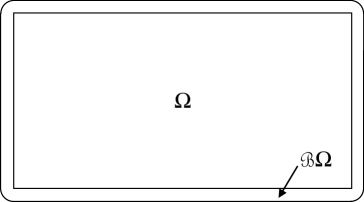
Figure 2.1: Typical domain for (1.1). $\mathbf{u}$ is prescribed in $\mathcal{B}\Omega$, and we solve for $\mathbf{u}$ in $\Omega$.

2.1 Nonlocal Diffusion Processes

The equation

$$u_{t}(\mathbf{x},t)=\mathcal{L}(u(\mathbf{x},t))$$ (2.2)

is an instance of a nonlocal p-Laplace equation for $p=2$, and has been used to model nonlocal diffusion processes, see [36], [28] and the references cited therein. In this setting, $u(\mathbf{x},t)\in\mathbb{R}$ is the density at the point $\mathbf{x}$ at time $t$ of some material, and we assume $C(\mathbf{x},\mathbf{x^{\prime}})=C(\mathbf{x}-\mathbf{x^{\prime}})$ is translation invariant. Then, $\int_{\mathbb{R}^{d}}C(\mathbf{x^{\prime}}-\mathbf{x})u(\mathbf{x^{\prime}},t)d\mathbf{x^{\prime}}$ is the rate at which material is arriving at $\mathbf{x}$ from all other points in $\textrm{supp}(C)$, and $-\int_{\mathbb{R}^{d}}C(\mathbf{x^{\prime}}-\mathbf{x})u(\mathbf{x},t)d\mathbf{x^{\prime}}$ is the rate at which material departs $\mathbf{x}$ for all other points in $\textrm{supp}(C)$ [37, 28].

In this interpretation of (1.1) the following restrictions are placed upon $C$ in $\mathcal{L}$. It is assumed that $C:\mathbb{R}^{d}\rightarrow\mathbb{R}$ is a nonnegative, radial, continuous function that is strictly positive in a ball of radius $\delta$ about $\mathbf{x}$ and zero elsewhere. Additionally, it is assumed that $\int_{\Omega}C(\mbox{\boldmath$\xi$})d\mbox{\boldmath$\xi$}~{}<~{}\infty$.

2.2 Nonlocal Solid Mechanics

The equation

$$\mathbf{u}_{tt}(\mathbf{x},t)=\mathcal{L}(\mathbf{u}(\mathbf{x},t))+\mathbf{b}(\mathbf{x})$$ (2.3)

is the linearized peridynamic equation [38, eqn. (56)]. The corresponding time-independent (“peristatic”) equilibrium equation is (1.1). Peridynamics is a nonlocal reformulation of continuum mechanics that is oriented toward deformations with discontinuities, see [38, 39, 40] and the references therein. In this context, $\mathbf{u}\in\mathbb{R}^{n}$ is the displacement field for the body $\Omega$, and $\mathbf{C}(\mathbf{x},\mathbf{x^{\prime}})$ is a stiffness tensor, also known as a micromodulus tensor.

In this interpretation of (1.1) the following restrictions are placed upon $\mathbf{C}$ in $\mathcal{L}$. It is assumed that $\mathbf{C}$ is integrable and strictly positive definite in the neighborhood of $\mathbf{x}$, $\mathcal{H}_{\mathbf{x}}$, defined as

$$\mathcal{H}_{\mathbf{x}}:=\{\mathbf{x^{\prime}}\in\mathbb{R}^{d}\;:\;\lVert\mathbf{x^{\prime}}-\mathbf{x}\rVert\leq\delta\},$$ (2.4)

where $\delta>0$ is called the horizon. These assumptions are made because they are sufficient to ensure material stability [38, pp. 191-194]. It is also assumed that $\mathbf{C}=\mathbf{0}$ for $\lVert\mathbf{x^{\prime}}-\mathbf{x}\rVert>\delta$. If the material is elastic, it follows that $\mathbf{C}(\mathbf{x},\mathbf{x^{\prime}})$ is symmetric (e.g., $\mathbf{C}(\mathbf{x},\mathbf{x^{\prime}})^{T}=\mathbf{C}(\mathbf{x},\mathbf{x^{\prime}})$). Further, it is assumed that $\mathbf{C}$ is symmetric with respect to its arguments (e.g., $\mathbf{C}(\mathbf{x},\mathbf{x^{\prime}})=\mathbf{C}(\mathbf{x^{\prime}},\mathbf{x})$). This follows from imposing that the integrand of (1.2) must be anti-symmetric in its arguments, e.g.,

$$\mathbf{C}(\mathbf{x},\mathbf{x^{\prime}})\,[\mathbf{u}(\mathbf{x^{\prime}})-\mathbf{u}(\mathbf{x})]=-\mathbf{C}(\mathbf{x^{\prime}},\mathbf{x})\,[\mathbf{u}(\mathbf{x})-\mathbf{u}(\mathbf{x^{\prime}})]$$

in accordance with Newton’s third law.

3 A Nonlocal Variational Formulation

Here we present a variational formulation of the nonlocal equation (1.1). For peridynamics, this was presented by Emmerich and Weckner in [41]. An analogous expression also appears in [38, eqn. (75)], as well as [25].

Our construction takes place on the domain under consideration and its nonlocal boundary, i.e., $\Omega\cup\mathcal{B}\Omega$. We define the nonlocal closure of $\Omega$ as follows:

$$\overline{\overline{\Omega}}:=\Omega\cup\mathcal{B}\Omega.$$

We will utilize the function space

$$V:=L_{2,0}^{n}(\overline{\overline{\Omega}})=\left\{\mathbf{v}\in L_{2}^{n}(\overline{\overline{\Omega}}):\mathbf{v}|_{\mathcal{B}\Omega}=\mathbf{0}\right\},$$ (3.1)

and the inner product

$$(\mathbf{u},\mathbf{v}):=\int_{\overline{\overline{\Omega}}}\mathbf{u}\,\mathbf{v}~{}d\mathbf{x}.$$

The weak formulation of (1.1) is the following: Given $\mathbf{b}(\mathbf{x})\in L_{2}^{n}(\Omega)$, find $\mathbf{u}(\mathbf{x})\in V$ such that

$$a(\mathbf{u},\mathbf{v})=(\mathbf{b},\mathbf{v})\qquad\forall\mathbf{v}\in V,$$ (3.2)

where

$$a(\mathbf{u},\mathbf{v}):=-\int_{\overline{\overline{\Omega}}}\left\{\int_{\overline{\overline{\Omega}}}\mathbf{C}(\mathbf{x},\mathbf{x^{\prime}})\,[\mathbf{u}(\mathbf{x^{\prime}})-\mathbf{u}(\mathbf{x})]~{}d\mathbf{x^{\prime}}\right\}\,\mathbf{v}(\mathbf{x})~{}d\mathbf{x}.$$ (3.3)

We assume that the iterated integral in (3.3) is finite:

$$-\int_{\overline{\overline{\Omega}}}\left\{\int_{\overline{\overline{\Omega}}}\mathbf{C}(\mathbf{x},\mathbf{x^{\prime}})\,[\mathbf{u}(\mathbf{x^{\prime}})-\mathbf{u}(\mathbf{x})]~{}d\mathbf{x^{\prime}}\right\}\,\mathbf{v}(\mathbf{x})~{}d\mathbf{x}<\infty,$$

and that $\mathbf{C}(\mathbf{x},\mathbf{x^{\prime}})\,[\mathbf{u}(\mathbf{x^{\prime}})-\mathbf{u}(\mathbf{x})]$ is anti-symmetric in its arguments. Combining these observations with Fubini’s Theorem gives the identity

$$-\int_{\overline{\overline{\Omega}}}\left\{\int_{\overline{\overline{\Omega}}}\mathbf{C}(\mathbf{x},\mathbf{x^{\prime}})\,[\mathbf{u}(\mathbf{x^{\prime}})-\mathbf{u}(\mathbf{x})]~{}d\mathbf{x^{\prime}}\right\}\,\mathbf{v}(\mathbf{x})~{}d\mathbf{x}=$$ (3.4)

$$\frac{1}{2}\int_{\overline{\overline{\Omega}}}\left\{\int_{\overline{\overline{\Omega}}}\mathbf{C}(\mathbf{x},\mathbf{x^{\prime}})\,[\mathbf{u}(\mathbf{x^{\prime}})-\mathbf{u}(\mathbf{x})][\mathbf{v}(\mathbf{x^{\prime}})-\mathbf{v}(\mathbf{x})]~{}d\mathbf{x}^{\prime}\right\}\,~{}d\mathbf{x}.$$

For the proof of well-posedness of the nonlocal BVP (3.2), we utilize the equivalent expression in (3.4) which induces the following bilinear form:

$$a(\mathbf{u},\mathbf{v})=\frac{1}{2}\int_{\overline{\overline{\Omega}}}\int_{\overline{\overline{\Omega}}}\mathbf{C}(\mathbf{x},\mathbf{x^{\prime}})\,[\mathbf{u}(\mathbf{x^{\prime}})-\mathbf{u}(\mathbf{x})]\,[\mathbf{v}(\mathbf{x^{\prime}})-\mathbf{v}(\mathbf{x})]~{}d\mathbf{x^{\prime}}~{}d\mathbf{x},$$ (3.5)

In §4.1, we will establish the coercivity of $a(u,u)$ in $V$ in the case of scalar functions, i.e., by setting $n=1$ in (3.1). The continuity of $a(u,v)$ in $L_{2}(\overline{\overline{\Omega}})$ follows from (4.24). Furthermore, $R(v):=(b,v)$ is a bounded linear functional on $L_{2}(\overline{\overline{\Omega}})$. Therefore, well-posedness of (3.2) follows from the Lax-Milgram Lemma; also see [25, Sec. 6].

In 1D with $\overline{\overline{\Omega}}:=[-\delta,1+\delta]$, the weak form (3.5) becomes

$$a(u,u)=\frac{1}{2}\int_{[-\delta,1+\delta]}\int_{[x-\delta,x+\delta]\cap[-\delta,1+\delta]}C(x,x^{\prime})\left(u(x^{\prime})-u(x)\right)^{2}dx^{\prime}dx,$$ (3.6)

where the limits of integration have been adjusted to account for the support of $C(x,x^{\prime})$, which is assumed to vanish if $\lVert x-x^{\prime}\rVert>\delta$. For this problem, the two-dimensional domain of integration is the parallelogram shown in Figure 3.1. For 2D and 3D problems, the domains of integration are four and six dimensional, respectively.

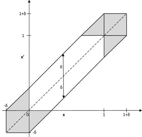
Figure 3.1: Domain of integration for a 1D problem where $\Omega=[0,1]$ and $\mathcal{B}\Omega=[-\delta,0]\cup[1,1+\delta]$. A nonlocal Dirichlet boundary condition is prescribed over $\mathcal{B}\Omega$. The grey region indicates the portion of the integration domain where either or both of $x$, $x^{\prime}$ lie outside $\Omega$.

4 Nonlocal Spectral Equivalence

The principle result of this section is Theorem 1, a condition number bound for the stiffness matrix arising from a finite element discretization of (3.3). We investigate the conditioning because it determines both the accuracy of the computed numerical solution, as well as the computational effort required by an iterative linear solver to produce the numerical solution. Quantifying the condition number bound is a necessary first step towards developing scalable preconditioners and optimal solvers for nonlocal models.

In the local setting, the classical condition number estimates rely on a Poincaré inequality and an inverse inequality for the lower and upper bound, respectively. Similarly to the local case, we develop a nonlocal Poincaré inequality to be used in the lower bound. We prove a nonlocal Poincaré inequality which is used to establish the coercivity of the underlying bilinear form. However, for condition number analysis, one needs a more refined Poincaré inequality which involves an explicit $\delta$-quantification. Such refined inequality requires substantially more involved analysis, which has been accomplished by the first author in the companion article [42].

The $\delta$-quantification is an essential feature in the nonlocal setting because the lower bound turns out to be dimension dependent, unlike in the local case. This dimensional dependence is induced by the neighborhood $\mathcal{H}_{x}$ (see (2.4)), which is $d$-dimensional in the nonlocal setting but zero-dimensional (a point) in the local setting. Dimension dependence in the Poincaré inequality is captured by $\delta^{m}$ (see §4.1) where the power $m$ exhibits a dimensional dependence (i.e., $m=m(d)$).

For the upper bound, we prove a direct estimate instead of an inverse inequality. Neither the upper bound estimate nor the Poincaré inequality requires discrete spaces. Hence, our estimate is valid in infinite dimensional function spaces, a stronger result than that for the local setting.

We investigate the effect of the horizon size $\delta$ on the conditioning of the underlying operators. Therefore, we reduce the analysis to the case $\mathbf{C}(\mathbf{x},\mathbf{x^{\prime}})=\chi_{\delta}(\mathbf{x}-\mathbf{x^{\prime}})$ where $\chi_{\delta}(\mathbf{x}-\mathbf{x^{\prime}})$ denotes the canonical kernel function whose only role is the representation of the neighborhood in (2.4) by a characteristic function. Namely,

$$\chi_{\delta}(\mathbf{x}-\mathbf{x^{\prime}}):=\left\{\begin{array}[]{cl}1,&\lVert\mathbf{x}-\mathbf{x}^{\prime}\rVert\leq\delta\\ 0,&\textrm{otherwise.}\end{array}\right.$$ (4.3)

Note that $\chi_{\delta}(\mathbf{x}-\mathbf{x^{\prime}})$ is a radial function, which describes isotropic materials [40]. For the remainder of this article, we will restrict our discussion to scalar problems. Namely, we set $n=1$ in (3.1) which yields, for instance, $\mathbf{u}(\mathbf{x})=u(\mathbf{x})$, $\mathbf{C}(\mathbf{x},\mathbf{x^{\prime}})=C(\mathbf{x},\mathbf{x^{\prime}})$, etc. Therefore, the bilinear form under consideration becomes

$$a(u,v)=\frac{1}{2}\int_{\overline{\overline{\Omega}}}\int_{\overline{\overline{\Omega}}}\chi_{\delta}(\mathbf{x}-\mathbf{x^{\prime}})[u(\mathbf{x^{\prime}})-u(\mathbf{x})][v(\mathbf{x^{\prime}})-v(\mathbf{x})]~{}d\mathbf{x^{\prime}}~{}d\mathbf{x}.$$ (4.4)

We state an important property of the canonical kernel which will be used in the upcoming proofs:

$$\int_{\overline{\overline{\Omega}}}\chi_{\delta}(\mathbf{x}-\mathbf{x^{\prime}})~{}d\mathbf{x}^{\prime}\leq w_{d}\delta^{d}\quad\mathbf{x}\in\overline{\overline{\Omega}},$$ (4.5)

where $w_{d}$ is the volume of the unit ball in $\mathbb{R}^{d}$. Note that the equality in (4.5) is attained when the neighborhood of $\mathbf{x}$, $\mathcal{H}_{\mathbf{x}}$ in (2.4), is entirely contained in $\overline{\overline{\Omega}}$, i.e., when $\mathbf{x}\in\Omega$.

4.1 Nonlocal Poincaré inequality

In order to establish the coercivity of $a(\cdot,\cdot)$, we prove a nonlocal Poincaré inequality.

Proposition 1

Let $\Omega\subset\mathbb{R}^{d}$ be a bounded domain and $u\in L_{2,0}(\overline{\overline{\Omega}})$. Then, there exists $\lambda_{Pncr}=\lambda_{Pncr}(\overline{\overline{\Omega}},\delta)>0$ such that

$$\lambda_{Pncr}\,\|u\|^{2}_{L_{2}(\overline{\overline{\Omega}})}\leq a(u,u)$$ (4.6)

Proof 1

The proof is an extension of the one given in [28, Prop. 2.5] for a similar bilinear form. We construct a finite covering for $\overline{\overline{\Omega}}$ using strips of width $\delta/2$ as follows:

$$S_{-1} := \{\mathbf{x}\in\mathcal{B}\Omega:\frac{\delta}{2}\leq\mathrm{dist}(\mathbf{x},\partial\Omega)\leq\delta\},$$ (4.7)

$$S_{0} := \{\mathbf{x}\in\mathcal{B}\Omega\setminus S_{-1}:\mathrm{dist}(\mathbf{x},S_{-1})\leq\frac{\delta}{2}\},$$ (4.8)

$$S_{1} := \{\mathbf{x}\in\Omega:\mathrm{dist}(\mathbf{x},\partial\Omega)\leq\frac{\delta}{2}\},$$ (4.9)

$$S_{j} := \{\mathbf{x}\in\Omega\setminus\bigcup_{k=1}^{j-1}S_{k}:\mathrm{dist}(\mathbf{x},S_{j-1})\leq\frac{\delta}{2}\},\quad j=1\ldots,l,$$ (4.10)

where $\mathrm{dist}$ denotes the shortest distance in the usual Euclidean sense. The number of strips covering $\Omega$ is $l=l(\overline{\overline{\Omega}},\delta)$.

We trivially have the following for $j=0,\ldots,l$:

$$\int_{\overline{\overline{\Omega}}}\int_{\overline{\overline{\Omega}}}\chi_{\delta}(\mathbf{x}-\mathbf{x^{\prime}})\,|u(\mathbf{x}^{\prime})-u(\mathbf{x})|^{2}~{}d\mathbf{x}^{\prime}d\mathbf{x}\geq\int_{S_{j}}\int_{S_{j-1}}\chi_{\delta}(\mathbf{x}-\mathbf{x^{\prime}})\,|u(\mathbf{x}^{\prime})-u(\mathbf{x})|^{2}~{}d\mathbf{x}^{\prime}d\mathbf{x}.$$

Using $|u(\mathbf{x})|^{2}=|u(\mathbf{x^{\prime}})-\{u(\mathbf{x^{\prime}})-u(\mathbf{x})\}|^{2}\leq 2\{|u(\mathbf{x^{\prime}})-u(\mathbf{x})|^{2}+|u(\mathbf{x^{\prime}})|^{2}\},$ a change in the order of integration, and the following result (obtained from (4.5))

$$\int_{S_{j}}\chi_{\delta}(\mathbf{x}-\mathbf{x^{\prime}})~{}d\mathbf{x}^{\prime}\leq w_{d}\delta^{d},$$

we obtain the following:

$$\int_{S_{j}}\int_{S_{j-1}}\chi_{\delta}(\mathbf{x}-\mathbf{x^{\prime}})\,|u(\mathbf{x}^{\prime})-u(\mathbf{x})|^{2}~{}d\mathbf{x}^{\prime}d\mathbf{x}$$

$$\geq \frac{1}{2}\int_{S_{j}}\int_{S_{j-1}}\chi_{\delta}(\mathbf{x}-\mathbf{x^{\prime}})\,|u(\mathbf{x})|^{2}~{}d\mathbf{x^{\prime}}d\mathbf{x}-\int_{S_{j}}\int_{S_{j-1}}\chi_{\delta}(\mathbf{x}-\mathbf{x^{\prime}})\,|u(\mathbf{x}^{\prime})|^{2}~{}d\mathbf{x^{\prime}}d\mathbf{x}$$

$$= \frac{1}{2}\int_{S_{j}}\left\{\int_{S_{j-1}}\chi_{\delta}(\mathbf{x}-\mathbf{x^{\prime}})~{}d\mathbf{x^{\prime}}\right\}\,|u(\mathbf{x})|^{2}~{}d\mathbf{x}-\int_{S_{j-1}}\left\{\int_{S_{j}}\chi_{\delta}(\mathbf{x}-\mathbf{x^{\prime}})d\mathbf{x}\right\}\,|u(\mathbf{x^{\prime}})|^{2}~{}d\mathbf{x^{\prime}}$$

$$\geq \frac{1}{2}\int_{S_{j}}\left\{\int_{S_{j-1}}\chi_{\delta}(\mathbf{x}-\mathbf{x^{\prime}})~{}d\mathbf{x^{\prime}}\right\}\,|u(\mathbf{x})|^{2}~{}d\mathbf{x}-w_{d}\,\delta^{d}\int_{S_{j-1}}|u(\mathbf{x}^{\prime})|^{2}~{}d\mathbf{x^{\prime}}$$

$$\geq \frac{1}{2}\,\min_{x\in\overline{S}_{j}}\int_{S_{j-1}}\chi_{\delta}(\mathbf{x}-\mathbf{x^{\prime}})~{}d\mathbf{x^{\prime}}\int_{S_{j}}|u(\mathbf{x})|^{2}~{}d\mathbf{x}-w_{d}\,\delta^{d}\,\int_{S_{j-1}}|u(\mathbf{x}^{\prime})|^{2}~{}d\mathbf{x}^{\prime}.$$

The function

$$F(\mathbf{x}):=\int_{S_{j-1}}\chi_{\delta}(\mathbf{x}-\mathbf{x^{\prime}})~{}d\mathbf{x^{\prime}},\quad\mathbf{x}\in\overline{S_{j}}$$

is continuous, which follows from continuity of the integral operator and the fact that $\chi_{\delta}(\mathbf{x}-\mathbf{x^{\prime}})$ is integrable. By construction of the covering, we have

$$S_{j-1}\cap B(\mathbf{x},\delta)\neq\emptyset,\quad\mathbf{x}\in S_{j},$$

where $B(\mathbf{x},\delta)$ is a ball of radius $\delta$ centered at $\mathbf{x}$. Hence, we obtain

$$F(\mathbf{x})=\text{measure}(\{\mathbf{x}\in\overline{S_{j}}:S_{j-1}\cap B(\mathbf{x},\delta)\})>0,\quad\mathbf{x}\in\overline{S_{j}}.$$

Therefore by continuity, $F(\mathbf{x})$ attains its infimum in $\overline{S_{j}}$ and we conclude that

$$\alpha_{j}:=\min_{\mathbf{x}\in\overline{S}_{j}}F(\mathbf{x})>0.$$

Consequently, we have the inequality:

$$\frac{\alpha_{j}}{4}\int_{S_{j}}|u(\mathbf{x})|^{2}~{}d\mathbf{x}\leq a(u,u)+w_{d}\,\delta^{d}\int_{S_{j-1}}|u(\mathbf{x^{\prime}})|^{2}~{}d\mathbf{x^{\prime}}.$$ (4.11)

From the boundary condition, we get

$$\int_{S_{-1}}|u(\mathbf{x})|^{2}~{}d\mathbf{x}=\int_{S_{0}}|u(\mathbf{x})|^{2}~{}d\mathbf{x}=0.$$

Moreover due to the boundary condition and (4.11), we get

$$\frac{\alpha_{1}}{4}\int_{S_{1}}|u(\mathbf{x})|^{2}~{}d\mathbf{x}\leq a(u,u)$$ (4.12)

For the cases $j=2,3$, we respectively have:

$$\frac{\alpha_{2}}{4}\int_{S_{2}}|u(\mathbf{x})|^{2}~{}d\mathbf{x} \leq a(u,u)+w_{d}\,\delta^{d}\int_{S_{1}}|u(\mathbf{x^{\prime}})|^{2}~{}d\mathbf{x^{\prime}}$$ (4.13)

$$\frac{\alpha_{3}}{4}\int_{S_{3}}|u(\mathbf{x})|^{2}~{}d\mathbf{x} \leq a(u,u)+w_{d}\,\delta^{d}\int_{S_{2}}|u(\mathbf{x^{\prime}})|^{2}~{}d\mathbf{x^{\prime}}.$$ (4.14)

To relate (4.14) to right-hand side of (4.13), multiply (4.13) by $(4\,w_{d}\,\delta^{d})/\alpha_{2}$:

$$\frac{\alpha_{3}}{4}\int_{S_{3}}|u(\mathbf{x})|^{2}~{}d\mathbf{x}\leq(1+\frac{4\,w_{d}\,\delta^{d}}{\alpha_{2}})~{}a(u,u)+\frac{4\,(w_{d}\,\delta^{d})^{2}}{\alpha_{2}}\int_{S_{1}}|u(\mathbf{x^{\prime}})|^{2}~{}d\mathbf{x^{\prime}}.$$ (4.15)

Then using (4.12), (4.15) becomes:

$$\frac{\alpha_{3}}{4}~{}\int_{S_{3}}|u(\mathbf{x})|^{2}~{}d\mathbf{x}\leq\left(1+\frac{4\,w_{d}\,\delta^{d}}{\alpha_{2}}+\frac{(4\,w_{d}\,\delta^{d})^{2}}{\alpha_{1}\,\alpha_{2}}\right)~{}a(u,u).$$

Continuing this process, we see the existence of a constant $c(\overline{\overline{\Omega}},\delta)$ satisfying:

$$\frac{\alpha_{j}}{4}~{}\int_{S_{j}}|u(\mathbf{x})|^{2}~{}d\mathbf{x}\leq c(\overline{\overline{\Omega}},\delta)~{}a(u,u),\quad j=-1,\ldots,l.$$ (4.16)

Adding (4.16) for $j=-1,\ldots,l$ and using the fact that the covering of $\overline{\overline{\Omega}}$ is composed of disjoint strips, i.e., $\overline{\overline{\Omega}}=\cup_{k=-1}^{l}S_{k},~{}~{}~{}S_{j}\cap S_{k}=\emptyset,~{}j\neq k$, we arrive at the coercivity result.

Remark 1

The coercivity proof in [28, Prop. 2.5] assumes a continuous kernel function. The coercivity proof we provide can be generalized to any nonnegative locally integrable radial kernel function which satisfies $C(r)>0$ on $(0,\delta)$ see the companion article [42, Lemma 2.4].

Remark 2

The above Poincaré type inequality can be established for general Dirichlet boundary conditions, i.e., $u\in L_{2}(\overline{\overline{\Omega}})$ with $u|_{\mathcal{B}\Omega}\neq 0$. In this case, the inequality statement reads as follows:

$$\lambda_{Pncr}(\overline{\overline{\Omega}},\delta)\,\|u\|^{2}_{L_{2}(\overline{\overline{\Omega}})}\leq a(u,u)+\int_{S_{-1}}|u(\mathbf{x})|^{2}~{}d\mathbf{x},$$ (4.17)

where $S_{-1}$ is the outermost strip of the covering of $\overline{\overline{\Omega}}$. Deducing a coercivity estimate from (4.17) seems impossible unless a zero nonloncal boundary condition is assumed. For mixed and Neumann type boundary conditions, see the companion paper [42, Remark 2.5].

Remark 3

Coercivity of the bilinear form has also been established in [25] under the condition (see [25, Eq. (6.1)]) that

$$\int_{\mathcal{B}\Omega}C(\mathbf{x},\mathbf{x^{\prime}})~{}d\mathbf{x^{\prime}}\geq c>0,\quad\mathbf{x}\in\Omega.$$ (4.18)

This condition is stringent because it assumes that all interior points interact directly with the nonlocal boundary $\mathcal{B}\Omega$, a situation only possible if the horizon $\delta$ is on the order of $|\Omega|$. For applications of practical interest especially in peridynamics, horizon is set to be $\delta\ll|\Omega|$ because problems with large $\delta$ are computationally intractable. The coercivity proof given in this article does not assume (4.18).

For the condition number analysis, $\delta$-quantification is essential. In the companion article [42], the first author gives a more refined nonlocal Poincaré inequality. Namely, for sufficiently small $\delta$:

$$\lambda_{refined}(\overline{\overline{\Omega}})\,\delta^{d+2}\|u\|^{2}_{L_{2}(\overline{\overline{\Omega}})}\leq a(u,u).$$ (4.19)

Note that $\lambda_{refined}$ does not depend on $\delta$. In order to see why $\lambda_{Pncr}(\overline{\overline{\Omega}},\delta)$ can be refined to a constant $\lambda_{refined}(\overline{\overline{\Omega}})$, we proceed with a 1D demonstration.

4.2 Demonstration of explicit $\delta$-dependence in the nonlocal Poincaré inequality

We demonstrate the lower bound in (4.19) by a 1D example. After enforcing a sufficient regularity assumption, we resort to a Taylor series expansion. For that purpose, we assume that $u\in C^{4}(\overline{\overline{\Omega}})$ with homogenous Dirichlet boundary conditions enforced on the nonlocal boundary $\mathcal{B}\Omega$. This demonstration is based on the desire to have the nonlocal bilinear form converge to its corresponding local (classical) bilinear form as $\delta\rightarrow 0$. For discussions of convergence of other nonlocal operators to their classical local counterparts, see [43, 44].

For the sake of clarity, we utilize the equivalent bilinear form below given in (3.4) so that the effect of the boundary condition can easily be seen. We accompany this with a change of variable as follows:

$$a(u,u) = -\int_{\overline{\overline{\Omega}}}\left\{\int_{\overline{\overline{\Omega}}\cap[x-\delta,x+\delta]}[u(x^{\prime})-u(x)]~{}dx^{\prime}\right\}u(x)~{}dx$$

$$= -\int_{\Omega}\left\{\int_{[x-\delta,x+\delta]}[u(x^{\prime})-u(x)]~{}dx^{\prime}\right\}u(x)~{}dx$$

$$= -\int_{\Omega}\left\{\int_{-\delta}^{\delta}[u(x+\varepsilon)-u(x)]~{}d\varepsilon\right\}u(x)~{}dx.$$

Using the Taylor expansion

$$u(x+\varepsilon) = u(x)+\frac{\varepsilon}{1!}\frac{du}{dx}(x)+\frac{\varepsilon^{2}}{2!}\frac{d^{2}u}{dx^{2}}(x)+\frac{\varepsilon^{3}}{3!}\frac{d^{3}u}{dx^{3}}(x)+\mathcal{O}(\varepsilon^{4}),$$

the integrand becomes:

$$[u(\varepsilon+x)-u(x)]u(x)=\varepsilon\frac{du}{dx}(x)u(x)+\frac{\varepsilon^{2}}{2!}\frac{d^{2}u}{dx^{2}}(x)u(x)+\frac{\varepsilon^{3}}{3!}\frac{d^{3}u}{dx^{3}}(x)u(x)+\mathcal{O}(\varepsilon^{4}).$$

Hence, we arrive at the following expression using $u|_{\partial\Omega}=0$ (due to $u|_{\mathcal{B}\Omega}=0$):

$$a(u,u) = -\int_{\Omega}\left\{\frac{\delta^{3}}{3}\frac{d^{2}u}{dx^{2}}(x)u(x)+\mathcal{O}(\delta^{5})\right\}~{}dx$$

$$= \frac{\delta^{3}}{3}\int_{\Omega}\frac{du}{dx}(x)\frac{du}{dx}(x)~{}dx+\mathcal{O}(\delta^{5}).$$

Now, denoting the local bilinear form by

$$\ell(u,u):=|u|_{H^{1}(\Omega)}^{2},$$

we connect the nonlocal and local bilinear forms:

$$a(u,u) = \frac{\delta^{3}}{3}~{}\ell(u,u)+\mathcal{O}(\delta^{5}).$$

Therefore, the scaled nonlocal bilinear form asymptotically converges to the local bilinear form:

$$3~{}\delta^{-3}~{}a(u,u)=\ell(u,u)+\mathcal{O}(\delta^{2}).$$ (4.20)

Using the nonlocal Poincaré inequality (4.6) and (4.20), we have

$$\lim_{\delta\rightarrow 0}~{}3~{}\lambda_{Pncr}(\overline{\overline{\Omega}},\delta)~{}\delta^{-3}~{}\lVert u\rVert_{L_{2}(\overline{\overline{\Omega}})}^{2}\leq\ell(u,u).$$

Therefore, for the left hand side to remain finite, we have to enforce that $\lambda_{Pncr}(\overline{\overline{\Omega}},\delta)=c(\overline{\overline{\Omega}})\,\delta^{m}$ with $m\geq 3$. We desire the largest possible lower bound in the nonlocal Poincaré inequality. This implies that $m=3$, which is in agreement with (4.19) and is observed numerically in 1D; see the experiments in §4.5.1.

4.3 An upper bound for $a(u,u)$

We prove the following dimension dependent estimate:

Lemma 1

Let $\overline{\overline{\Omega}}\subset\mathbb{R}^{d}$ be bounded and $u\in L_{2}(\overline{\overline{\Omega}})$. Then, there exists $\overline{\lambda}>0$ independent of $\overline{\overline{\Omega}}$ and $\delta$ such that

$$a(u,u)\leq\overline{\lambda}\;\delta^{d}\;\lVert u\rVert_{L_{2}(\overline{\overline{\Omega}})}^{2}.$$ (4.21)

Proof 2

Using $(u(\mathbf{x^{\prime}})-u(\mathbf{x}))^{2}\leq 2(u(\mathbf{x^{\prime}})^{2}+u(\mathbf{x})^{2})$, we get

$$a(u,u)\leq\int_{\overline{\overline{\Omega}}}\int_{\overline{\overline{\Omega}}}\chi_{\delta}(\mathbf{x}-\mathbf{x^{\prime}})(u^{2}(\mathbf{x})+u^{2}(\mathbf{x^{\prime}}))~{}d\mathbf{x^{\prime}}\,d\mathbf{x}.$$ (4.22)

Furthermore, by a change in the order of integration and the fact that $\chi_{\delta}(\mathbf{x}-\mathbf{x^{\prime}})$ is an even function, one gets

$$\int_{\overline{\overline{\Omega}}}\int_{\overline{\overline{\Omega}}}\chi_{\delta}(\mathbf{x}-\mathbf{x^{\prime}})u^{2}(\mathbf{x})~{}d\mathbf{x^{\prime}}\,d\mathbf{x}=\int_{\overline{\overline{\Omega}}}\int_{\overline{\overline{\Omega}}}\chi_{\delta}(\mathbf{x}-\mathbf{x^{\prime}})u^{2}(\mathbf{x^{\prime}})~{}d\mathbf{x^{\prime}}\,d\mathbf{x}.$$ (4.23)

Then using (4.23), (4.22) becomes:

$$a(u,u)\leq 2\int_{\overline{\overline{\Omega}}}\int_{\overline{\overline{\Omega}}}\chi_{\delta}(\mathbf{x}-\mathbf{x^{\prime}})\,u^{2}(\mathbf{x})~{}d\mathbf{x^{\prime}}\,d\mathbf{x}.$$

Using (4.5), we immediately have the upper bound:

$$2\int_{\overline{\overline{\Omega}}}\int_{\overline{\overline{\Omega}}}\chi_{\delta}(\mathbf{x}-\mathbf{x^{\prime}})\,u^{2}(\mathbf{x})~{}d\mathbf{x^{\prime}}\,d\mathbf{x} \leq 2w_{d}\,\delta^{d}~{}\|u\|_{L_{2}(\overline{\overline{\Omega}})}^{2}$$

$$=: \overline{\lambda}\,\delta^{d}~{}\|u\|_{L_{2}(\overline{\overline{\Omega}})}^{2}.$$

Remark 4

The upper bound is sharp; see the companion article [42, Sect. 4]. We also numerically demonstrate the numerical sharpness of the upper bound; see §4.5.

Remark 5

A proof similar to that of Lemma (1) can be given to show the boundedness of the bilinear form with an explicit constant. Namely,

$$|a(u,v)|\leq 2\,w_{d}\,\delta^{d}\,\|u\|_{L_{2}(\overline{\overline{\Omega}})}\|v\|_{L_{2}(\overline{\overline{\Omega}})}.$$ (4.24)

Also see the companion article [42] for the boundedness of the bilinear form for general kernel functions.

4.4 The Conditioning of the Stiffness Matrix $K$

Combining the refined nonlocal Poincaré inequality (4.19) and the upper bound (4.21), we arrive at a condition number estimate.

Theorem 1

For sufficiently small $\delta$, the following spectral equivalence holds:

$$\lambda_{refined}(\overline{\overline{\Omega}})~{}\delta^{d+2}\leq\frac{a(u,u)}{\lVert u\rVert_{L_{2}(\overline{\overline{\Omega}})}^{2}}\leq\overline{\lambda}~{}\delta^{d},\quad u\in L_{2,0}(\overline{\overline{\Omega}}).$$ (4.25)

Let $K$ be the stiffness matrix produced by discretizing $a(u,u)$. Then, the condition number of $K$ has the bound:

$$\kappa(K)\lesssim\delta^{-2}.$$ (4.26)

The spectral equivalence (4.25) enables us to construct an $h$ independent upper bound for the condition number.

Note that the condition number of the stiffness matrix also depends upon the mesh size $h$. As an illustration, consider that the nonlocal bilinear form $a(u,u)$ must converge to the corresponding local bilinear form in the limit $\delta\rightarrow 0$, as demonstrated in §4.2, and that the condition number of the associated local stiffness matrix varies with $h^{-2}$. Thus, the bound in (4.26) is not tight in this limit, but allows us to investigate the highly nonlocal regime $h\ll\delta$, which is our principle interest. For an alternative approach to quantifying mesh-dependence in the conditioning of nonlocal models, see [33].

		Piecewise Constant Shape Functions			Piecewise Linear Shape Functions
$1/h$	$1/\delta$	$\lambda_{\min}$	$\lambda_{\max}$	Condition #	$\lambda_{\min}$	$\lambda_{\max}$	Condition #
2000	20	1.94E-07	6.07E-05	3.13E+02	1.94E-07	6.07E-05	3.13E+02
4000	20	9.69E-08	3.04E-05	3.13E+02	9.69E-08	3.04E-05	3.14E+02
8000	20	4.84E-08	1.52E-05	3.14E+02	4.84E-08	1.52E-05	3.14E+02

(a) Fixed $\delta$, vary $h$.

		Piecewise Constant Shape Functions			Piecewise Linear Shape Functions
$1/h$	$1/\delta$	$\lambda_{\min}$	$\lambda_{\max}$	Condition #	$\lambda_{\min}$	$\lambda_{\max}$	Condition #
8000	20	4.84E-08	1.52E-05	3.15E+02	4.84E-08	1.52E-05	3.14E+02
8000	40	6.24E-09	7.61E-06	1.22E+03	6.24E-09	7.60E-06	1.22E+03
8000	80	7.92E-10	3.80E-06	4.80E+03	7.91E-10	3.80E-06	4.80E+03

(b) Fixed $h$, vary $\delta$.

Table 4.1: Condition number for $K$ in 1D for (a) fixed $\delta$, allowing $h$ to vary, and (b) fixed $h$, allowing $\delta$ to vary, for both piecewise constant and linear shape functions. We see that the conditioning is apparently not strongly influenced by the choice of shape function. This data is plotted in Figures 4.1.

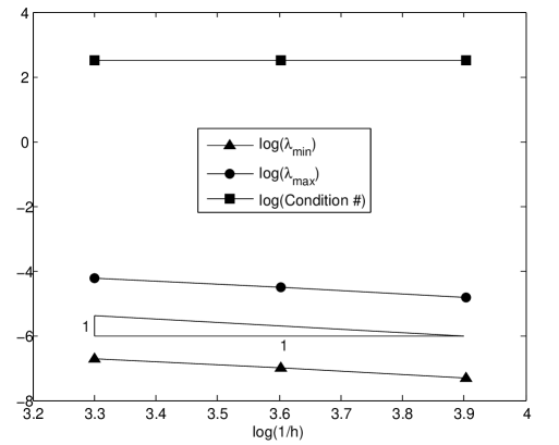
(a) Fixed $\delta$, vary $h$.

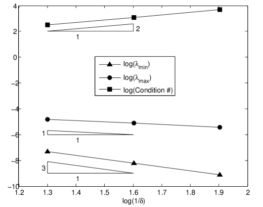
(b) Fixed $h$, vary $\delta$.

Figure 4.1: Condition number for $K$ in 1D for (a) fixed $\delta$, allowing $h$ to vary, and (b) fixed $h$, allowing $\delta$ to vary. The condition number is only weakly $h$-dependent, but varies with $\delta^{-2}$. These figures are plotted from data in Table 4.1. The plots for piecewise linear and piecewise constant shape functions are identical.

4.5 Numerical Verification of Condition Number by a Finite Element Formulation

For all computational results in this article, we let $\Omega=[0,1]^{d}$ be the unit $d$-cube, where $d$ is the spatial dimension, with $\overline{\overline{\Omega}}=[-\delta,1+\delta]^{d}$ the nonlocal closure. We impose the Dirichlet boundary condition $u=0$ on $\mathcal{B}\Omega=\overline{\overline{\Omega}}\backslash\Omega$. We use a conforming triangulation $\mathcal{T}_{h}$ where each element $E$ of $\mathcal{T}_{h}$ is a $d$-cube with a side length $h>0$. Consequently, each element in 1D, 2D, and 3D is a line segment of length $h$, a square of area $h^{2}$, and a cube of volume $h^{3}$, respectively. Let $V_{h}\subset V$ be a finite dimensional subspace of $V$ from (3.1). We use a Galerkin finite element formulation of (3.2):

$$a(u_{h},v_{h})=(b,v_{h})\qquad\forall v_{h}\in V_{h},$$ (4.27)

with Dirichlet boundary condition $u_{h}=0$ on $\mathcal{B}\Omega$, where $V_{h}$ is the space of piecewise constant or piecewise linear shape functions on the mesh $\mathcal{T}_{h}$, and where we employ the canonical kernel function $\chi_{\delta}$ from (4.3). We denote by $K$ the stiffness matrix arising from the left-hand side of (4.27). To verify our theoretical results we numerically determine the ratio of the largest and smallest eigenvalues of $K$, defining the condition number of the problem.

$1/h$	$1/\delta$	$\lambda_{\min}$	$\lambda_{\max}$	Condition #
50	10	2.95E-07	1.40E-05	4.77E+01
100	10	7.11E-08	3.54E-06	4.97E+01
200	10	1.75E-08	8.86E-07	5.05E+01

(a) Fixed $\delta$, vary $h$.

$1/h$	$1/\delta$	$\lambda_{\min}$	$\lambda_{\max}$	Condition #
200	10	1.75E-08	8.86E-07	5.05E+01
200	20	1.17E-09	2.22E-07	1.90E+02
200	40	7.63E-11	5.50E-08	7.21E+02

(b) Fixed $h$, vary $\delta$.

Table 4.2: Condition number for $K$ in 2D using piecewise constant shape functions for (a) fixed $\delta$, allowing $h$ to vary, and (b) fixed $h$, allowing $\delta$ to vary. This data is plotted in Figure 4.2.

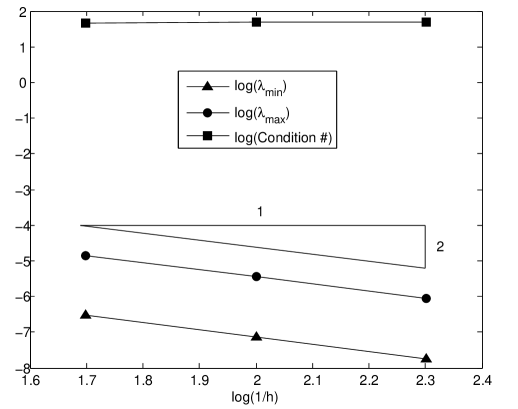
(a) Fixed $\delta$, vary $h$.

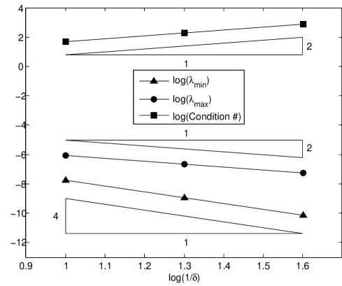
(b) Fixed $h$, vary $\delta$.

Figure 4.2: Condition number for $K$ in 2D for (a) fixed $\delta$, allowing $h$ to vary, and (b) fixed $h$, allowing $\delta$ to vary. The condition number is only weakly h-dependent, but varies with $\delta^{-2}$. These figures are plotted from data in Table 4.2.

4.5.1 Results in One Dimension

Results in this section appear in Tables 4.1 and Figures 4.1, where we consider the $h\ll\delta$ regime. We show results for both piecewise constant and piecewise linear shape functions to verify that the choice of shape function apparently does not influence the conditioning of the discrete system. We first compute the condition number of $K$ for different $h$ while holding $\delta$ fixed, and observe that the condition number of $K$ is only weakly $h$-dependent. The minimum and the maximum eigenvalues depend linearly on $h$, with a slope of nearly unity. We then compute the condition number of $K$ for different values of $\delta$ while holding $h$ fixed, and observe that the condition number varies with $\delta^{-2}$. Further, the maximum eigenvalue is proportional to $\delta$, in agreement with Lemma 1. Lastly, the minimum eigenvalue varies as $\delta^{3}$, in agreement with (4.19) and our finding of $m=3$ in §4.2. This suggests that, in one dimension, we should redefine $C(x,x^{\prime})$ in (4.3) as

$$C(x,x^{\prime})=\left\{\begin{array}[]{cl}\delta^{-3},&\lVert x-x^{\prime}\rVert\leq\delta\\ 0,&\textrm{otherwise.}\end{array}\right.,$$

for consistency with the weak form of the classical (local) Laplace operator in the limit $\delta\rightarrow 0$.

4.5.2 Results in Two Dimensions

Results in this section appear in Tables 4.2 and Figures 4.2. We consider only piecewise constant shape functions in 2D. We first compute the condition number of $K$ for different $h$ while holding $\delta$ fixed, and observe that minimum and maximum eigenvalues depend linearly on $h$ with a slope of approximately two, and again the condition number of $K$ depends only weakly upon the mesh size. We then compute the condition number of $K$ for different values of $\delta$ while holding $h$ fixed, and observe that the condition number again varies as $\delta^{-2}$, in agreement with (4.26). Further, the maximum eigenvalue is proportional to $\delta^{2}$ in agreement with Lemma 1, and the minimum eigenvalue is proportional to $\delta^{4}$ in agreement with (4.19).

5 A Nonlocal Two-Domain Problem

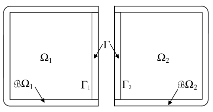
Figure 5.1: A nonlocal two-domain problem. This is a decomposition of the domain $\Omega$ in Figure 2.1 into overlapping subdomains $\Omega^{(1)}$, $\Omega^{(2)}$, and $\mathcal{B}\Omega$ into overlapping nonlocal boundaries $\mathcal{B}\Omega_{1}$, $\mathcal{B}\Omega_{2}$. Note that the interface $\Gamma$ is $d=2$-dimensional.

We will construct a weak (variational) formulation for nonlocal domain decomposition. We first identify the pieces of the domain for this decomposition. Consider the domain in Figure 5.1. The nonlocal boundary of $\Omega$, $\mathcal{B}\Omega$, is defined to be the closed region of thickness $\delta$ surrounding $\Omega$. Let $\Gamma$ be the open region corresponding to the interface between the two overlapping open subdomains $\Omega^{(1)}$ and $\Omega^{(2)}$. We define the overlapping subdomains $\Omega^{(i)},~{}~{}i=1,2$, as the following:

$$\Omega^{(i)}:=\Omega_{i}\cup\Gamma\cup\Gamma_{i},$$

where $\Gamma_{i}$ is the open line segment adjacent to $\Omega_{i}$ and $\Gamma$. Let $\mathcal{B}\Omega_{i}$ be the nonlocal closed boundary of $\Omega_{i}$ that intersects $\mathcal{B}\Omega$. The main domain decomposition contributions of this article, namely, the equivalence of the one-domain weak and two-domain weak forms will be proved next.

5.1 Two-Domain Variational Form

We present a two-domain weak formulation of (3.2) and prove its equivalence to the original single-domain formulation (3.2). We define the spaces, $i=1,2$,

$$V^{(i)} :=\left\{v\in L_{2}(\overline{\overline{\Omega^{(i)}}})\;:\;v|_{\mathcal{B}\Omega_{i}}=0\right\},$$ (5.1)

$$V^{(i),0} :=\left\{v\in L_{2}(\overline{\overline{\Omega^{(i)}}})\;:\;v|_{\mathcal{B}\Omega_{i}\cup\Gamma\cup\Gamma_{i}}=0\right\},$$

$$\Lambda :=\left\{\mu\in L_{2}(\Gamma):\mu=v|_{\Gamma}~{}\text{for some suitable}~{}v\in L_{2,0}(\overline{\overline{\Omega}})\right\}.$$

We can reduce the outer domain of integration in the bilinear form from $\overline{\overline{\Omega}}$ to $\Omega$ by taking advantage of the zero Dirichlet boundary condition. Namely,

$$a(u,v) = -\int_{\overline{\overline{\Omega}}}\left\{\int_{\overline{\overline{\Omega}}}\chi_{\delta}(\mathbf{x}-\mathbf{x^{\prime}})~{}[u(\mathbf{x^{\prime}})-u(\mathbf{x})]~{}d\mathbf{x^{\prime}}\right\}~{}v(\mathbf{x})~{}d\mathbf{x}$$ (5.2)

$$= -\int_{\Omega}\left\{\int_{\overline{\overline{\Omega}}}\chi_{\delta}(\mathbf{x}-\mathbf{x^{\prime}})~{}[u(\mathbf{x^{\prime}})-u(\mathbf{x})]~{}d\mathbf{x^{\prime}}\right\}~{}v(\mathbf{x})~{}d\mathbf{x},\quad v\in V.$$

Therefore, our construction is based on the reduced bilinear form (5.2). We further define a bilinear form $a_{\Omega^{(i)}}(u,v):V\times V\rightarrow\mathbb{R}$ as follows:

$$a_{\Omega^{(i)}}(u,v) := -\int_{\Omega_{i}}\left\{\int_{\Omega^{(i)}\cup\mathcal{B}\Omega_{i}}\chi_{\delta}(\mathbf{x}-\mathbf{x^{\prime}})~{}[u(\mathbf{x^{\prime}})-u(\mathbf{x})]~{}d\mathbf{x^{\prime}}\right\}~{}v(\mathbf{x})~{}d\mathbf{x}$$ (5.3)

$$-\frac{1}{2}\int_{\Gamma}\left\{\int_{\overline{\overline{\Omega}}}\chi_{\delta}(\mathbf{x}-\mathbf{x^{\prime}})~{}[u(\mathbf{x^{\prime}})-u(\mathbf{x})]~{}d\mathbf{x^{\prime}}\right\}~{}v(\mathbf{x})~{}d\mathbf{x}.$$

We utilize the following notation to suppress the integrals in (5.3):

$$a_{\Omega_{i}}(u,v) := -\int_{\Omega_{i}}\left\{\int_{\Omega^{(i)}\cup\mathcal{B}\Omega_{i}}\chi_{\delta}(\mathbf{x}-\mathbf{x^{\prime}})~{}[u(\mathbf{x^{\prime}})-u(\mathbf{x})]~{}d\mathbf{x^{\prime}}\right\}~{}v(\mathbf{x})~{}d\mathbf{x}$$ (5.4)

$$a_{\Gamma}(u,v) := -\int_{\Gamma}\left\{\int_{\overline{\overline{\Omega}}}\chi_{\delta}(\mathbf{x}-\mathbf{x^{\prime}})~{}[u(\mathbf{x^{\prime}})-u(\mathbf{x})]~{}d\mathbf{x^{\prime}}\right\}~{}v(\mathbf{x})~{}d\mathbf{x}$$ (5.5)

We can now represent the bilinear form (5.3) as:

$$a_{\Omega^{(i)}}(u,v)=\frac{1}{2}~{}a_{\Gamma}(u,v)+a_{\Omega_{i}}(u,v).$$

Remark 6

The test function $v_{i}=v|_{\Omega_{i}}\in V^{(i),0},~{}i=1,2$ has its support only in $\Omega_{i}$ not $\Omega^{(i)}$. Hence, we may reduce the bilinear form (5.3) to

$$a_{\Omega^{(i)}}(u^{(i)},v_{i})=a_{\Omega_{i}}(u^{(i)},v_{i}).$$ (5.6)

Although, $a_{\Gamma}(u^{(i)},v_{i})$ may appear to create a coupling between the subdomains, no such coupling exists because $v_{i}$ vanishes on $\Gamma$. Therefore, subdomain condition (5.7a) is an expression only for subdomain $\Omega^{(i)}$.

Now, we state the two-domain weak form following the notation of [16]: Find $u^{(i)}\in V^{(i)}$, $i=1,2$:

$$a_{\Omega^{(i)}}(u^{(i)},v_{i}) =(b,v_{i})_{\Omega_{i}} \forall v_{i}\in V^{(i),0},$$ (5.7a)

$$u^{(1)} =u^{(2)} \mbox{ on }\overline{\Gamma},$$ (5.7b)

$$\sum_{i=1,2}a_{\Omega^{(i)}}(u^{(i)},\mathcal{R}^{(i)}\mu) =(b,\mu)_{\Gamma}+\sum_{i=1,2}(b,\mathcal{R}^{(i)}\mu)_{\Omega_{i}} \forall\mu\in\Lambda.$$ (5.7c)

where $\mathcal{R}^{(i)}$ denotes any possible extension operator from $L_{2}(\Gamma)$ to $V^{(i)}$. An extension operator $\mathcal{R}^{(i)}:L_{2}(\Gamma)\rightarrow V^{(i)}$ is defined to be an operator which satisfies $(\mathcal{R}^{(i)}\eta)|_{\Gamma}=\eta$ for $\eta\in L_{2}(\Gamma).$ Next, we will show that the one- and two-domain weak forms are equivalent. The proof for the local case can be found in [16, Lemma 1.2.1].

Lemma 2

The problems (3.2) and (5.7) are equivalent.

Proof 3

$\eqref{eq:pdEquMotionWeak}\Rightarrow\eqref{eq:2DomainPD}:$
Let $u^{(i)}=u|_{\Omega^{(i)}}\in V^{(i)}$ and $v_{i}=v|_{\Omega_{i}}\in V^{(i),0},~{}i=1,2$. Extend these functions by zero extension;

$$\theta^{(i)}u^{(i)} := \left\{\begin{array}[]{ll}u^{(i)},&\text{in}~{}\Omega^{(i)}\\ 0,&\text{otherwise}\end{array}\right.$$

$$\theta_{i}v_{i} := \left\{\begin{array}[]{ll}v_{i},&\text{in}~{}\Omega_{i}\\ 0,&\text{otherwise}.\end{array}\right.$$

By LHS of (3.2) and using $v_{i}|_{\Gamma}=0$:

$$a(\theta^{(i)}u^{(i)},\theta_{i}v_{i}) = -\int_{\Omega}\left\{\int_{\overline{\overline{\Omega}}}\chi_{\delta}(\mathbf{x}-\mathbf{x^{\prime}})~{}[\theta^{(i)}u^{(i)}(\mathbf{x^{\prime}})-\theta^{(i)}u^{(i)}(\mathbf{x})]~{}d\mathbf{x^{\prime}}\right\}~{}\theta_{i}v_{i}(\mathbf{x})~{}d\mathbf{x}$$

$$= a_{\Omega_{i}}(u^{(i)},v_{i})$$

$$= \frac{1}{2}~{}a_{\Gamma}(u^{(i)},v_{i})+a_{\Omega_{i}}(u^{(i)},v_{i})$$

$$= a_{\Omega^{(i)}}(u^{(i)},v_{i})$$

By RHS of (3.2),

$$(b,\theta_{i}v_{i})=(b,v_{i})_{\Omega_{i}}.$$

Hence, (5.7a) is satisfied. (5.7b) is trivially satisfied.

Further, for $\mu\in\Lambda$ define the function $\mathcal{R}\mu$ as:

$$\mathcal{R}\mu:=\left\{\begin{array}[]{ll}\mathcal{R}^{(1)}\mu,&\mbox{in }\Omega^{(1)}\\ \mathcal{R}^{(2)}\mu,&\mbox{in }\Omega^{(2)}.\end{array}\right.\$$

Since $\mathcal{R}\mu$ lives only in $\Omega_{1}\cup\Gamma_{1}\cup\Gamma\cup\Gamma_{2}\cup\Omega_{2}$, it vanishes on $\mathcal{B}\Omega$. Therefore, $\mathcal{R}\mu\in V$.

From (3.2), partitioning the outer integral and using $\mathcal{R}^{(1)}\mu=\mathcal{R}^{(2)}\mu=\mu$ on $\Gamma$, we obtain the LHS of (5.7c):

$$a(u,\mathcal{R}\mu) = \frac{1}{2}~{}a_{\Gamma}(u^{(1)},\mu)+\frac{1}{2}~{}a_{\Gamma}(u^{(2)},\mu)+\sum_{i=1,2}a_{\Omega_{i}}(u^{(i)},\mathcal{R}^{(i)}\mu)$$

$$= \frac{1}{2}~{}a_{\Gamma}(u^{(1)},\mathcal{R}^{(1)}\mu)+\frac{1}{2}~{}a_{\Gamma}(u^{(2)},\mathcal{R}^{(2)}\mu)+\sum_{i=1,2}a_{\Omega_{i}}(u^{(i)},\mathcal{R}^{(i)}\mu)$$

$$= a_{\Omega^{(1)}}(u^{(1)},\mathcal{R}^{(1)}\mu)+a_{\Omega^{(2)}}(u^{(2)},\mathcal{R}^{(2)}\mu).$$

Likewise, from (3.2) and partitioning the integral, we obtain the RHS of (5.7c):

$$(b,\mathcal{R}\mu)_{\Omega}=(b,\mathcal{R}^{(1)}\mu)_{\Omega_{1}}+(b,\mathcal{R}^{(2)}\mu)_{\Omega_{2}}+(b,\mu)_{\Gamma}.$$

Hence, we obtain the transmission condition (5.7c).
$\eqref{eq:2DomainPD}\Rightarrow\eqref{eq:pdEquMotionWeak}:$
Let $u_{\Gamma}:=u^{(1)}|_{\Gamma}$ (due to (5.7b), we also have $u_{\Gamma}=u^{(2)}|_{\Gamma}$) and

$$u:=\left\{\begin{array}[]{ll}u^{(1)},&\mbox{in }\Omega_{1}\\ u^{(2)},&\mbox{in }\Omega_{2}\\ u_{\Gamma},&\mbox{in }\Gamma.\\ \end{array}\right.\$$ (5.13)

We partition the outer integral, use (5.13) and the transmission condition (5.7b). Then, for $v\in V$, LHS in (3.2) becomes the following:

$$a(u,v) = \frac{1}{2}~{}a_{\Gamma}(u,v)+\frac{1}{2}~{}a_{\Gamma}(u,v)+\sum_{i=1,2}a_{\Omega_{i}}(u,v)$$ (5.14)

$$= \frac{1}{2}~{}a_{\Gamma}(u_{\Gamma},v)+\frac{1}{2}~{}a_{\Gamma}(u_{\Gamma},v)+\sum_{i=1,2}a_{\Omega_{i}}(u^{(i)},v)$$

$$= \frac{1}{2}~{}a_{\Gamma}(u^{(1)},v)+\frac{1}{2}~{}a_{\Gamma}(u^{(2)},v)+\sum_{i=1,2}a_{\Omega_{i}}(u^{(i)},v)$$

$$= \sum_{i=1,2}a_{\Omega^{(i)}}(u^{(i)},v).$$

Let $\mu:=v|_{\Gamma}$. Then, $v-\mathcal{R}^{(i)}\mu\in V^{(i),0}$. First, we add and subtract $\mathcal{R}^{(i)}\mu$ to the second slot of the bilinear form in (5.14) and apply the domain conditions (5.7a) for $v-\mathcal{R}^{(i)}\mu$. Then, we apply the transmission condition (5.7c) and use $v|_{\Gamma}=\mu$. Hence, we arrive at the RHS in (3.2):

$$\sum_{i=1,2}a_{\Omega^{(i)}}(u^{(i)},v) = \sum_{i=1,2}a_{\Omega^{(i)}}(u^{(i)},v-\mathcal{R}^{(i)}\mu)+\sum_{i=1,2}a_{\Omega^{(i)}}(u^{(i)},\mathcal{R}^{(i)}\mu)$$

$$= \sum_{i=1,2}(b,v-\mathcal{R}^{(i)}\mu)_{\Omega_{i}}+\sum_{i=1,2}a_{\Omega^{(i)}}(u^{(i)},\mathcal{R}^{(i)}\mu)$$

$$= \sum_{i=1,2}(b,v-\mathcal{R}^{(i)}\mu)_{\Omega_{i}}+(b,\mu)_{\Gamma}+\sum_{i=1,2}(b,\mathcal{R}^{(i)}\mu)_{\Omega_{i}}$$

$$= (b,\mu)_{\Gamma}+\sum_{i=1,2}(b,v)_{\Omega_{i}}$$

$$= (b,v).$$

6 Towards Nonlocal Substructuring

Here we write out the linear algebraic representations arising from the two-domain weak form (5.7), identifying the discrete subdomain equations and transmission conditions. We then construct a nonlocal Schur complement, discuss its condition number as a function of $h$, $\delta$, and provide supporting numerical experiments.

6.1 Linear Algebraic Representations

We consider a finite element discretization of (5.7). Letting $V_{h}^{(i)}$ denote the finite element space corresponding to $\Omega^{(i)}$, we define:

$$V_{h}^{(i),0} := \left\{v_{h}\in V_{h}^{(i)}:~{}v_{h}|_{\mathcal{B}\Omega_{i}\cup\Gamma\cup\Gamma_{i}}=0\right\}$$

$$\Lambda_{h} := \left\{\mu_{h}\in L_{2}(\Gamma):~{}\mu_{h}=v_{h}|_{\Gamma}~{}\text{for some suitable}~{}v_{h}\in V_{h}\right\}.$$

Here, $\Lambda_{h}$ denotes a finite element discretization of $L_{2}(\Gamma)$. We see that the finite element formulation of (5.7) can be written as:

$$a_{\Omega^{(i)}}(u_{h}^{(i)},v_{i,h}) =(b,v_{i,h})_{\Omega_{i}} \forall v_{i,h}\in V_{h}^{(i),0},$$ (6.1a)

$$u_{h}^{(1)} =u_{h}^{(2)} \mbox{ on }\overline{\Gamma},$$ (6.1b)

$$\sum_{i=1,2}a_{\Omega^{(i)}}(u_{h}^{(i)},\mathcal{R}_{h}^{(i)}\mu_{h}) =(b,\mu_{h})_{\Gamma}+\sum_{i=1,2}(b,\mathcal{R}_{h}^{(i)}\mu_{h})_{\Omega_{i}} \forall\mu_{h}\in\Lambda_{h}.$$ (6.1c)

where $\mathcal{R}_{h}^{(i)}$ denotes any possible extension operator from $\Gamma_{h}$ to $V_{h}^{(i)}$. Following standard practice, we take these extension operators to be the finite element interpolant, which is defined to be equal to $\mu_{h}$ at the nodes in the thick interface $\Gamma$ and zero on the internal nodes of $\Omega_{i}$. If we number nodes in $\Omega_{1}$ first, nodes in $\Omega_{2}$ second, and nodes in $\Gamma$ last, we will arrive at a global stiffness matrix that takes the traditional block arrowhead form:

$$K=\left[\begin{array}[]{ccc}K_{11}&0&K_{1\Gamma}\\ 0&K_{22}&K_{2\Gamma}\\ K_{\Gamma 1}&K_{\Gamma 2}&K_{\Gamma\Gamma}\\ \end{array}\right]\left[\begin{array}[]{c}u_{1}\\ u_{2}\\ u_{\Gamma}\\ \end{array}\right]=\left[\begin{array}[]{c}f_{1}\\ f_{2}\\ f_{\Gamma}\\ \end{array}\right].$$ (6.11)

The first two block rows of the matrix in (6.11) arise from discretizing (6.1a), and the last block row arises from discretizing (6.1c).

6.2 Discrete Energy Minimizing Extension and the Schur Complement Conditioning

In order to study the conditioning of the Schur complement in the nonlocal setting, we define an analog of the discrete harmonic extension in the local case.

Definition 1

For a given $q\in\Lambda_{h}$, $E_{i}:\Lambda_{h}\rightarrow V_{h}^{(i)}$ defines a discrete energy minimizing extension into $\Omega_{i}$, if

$$E_{i}(q)|_{\Gamma} = q,$$ (6.12)

$$a_{i}(E_{i}(q),v) = 0,\quad v\in V_{h}^{(i),0},$$

where $a_{i}(\cdot,\cdot)$ denotes the bilinear form restricted to $\overline{\overline{\Omega^{(i)}}}$. Namely,

$$a_{i}(u,v)=\int_{\overline{\overline{\Omega^{(i)}}}}\left\{\int_{\overline{\overline{\Omega^{(i)}}}}\chi_{\delta}(\mathbf{x}-\mathbf{x^{\prime}})~{}[u(\mathbf{x^{\prime}})-u(\mathbf{x})]~{}d\mathbf{x^{\prime}}\right\}~{}v(\mathbf{x})~{}d\mathbf{x}.$$

The energy minimizing extension $E_{i}(q)$ of $q$ defines a canonical bilinear form $s_{i}(q,q):\Lambda_{h}\times\Lambda_{h}\rightarrow\mathbb{R}$ that is associated to the interface $\Gamma$ whose discretization corresponds to the subdomain Schur complement matrix $S^{(i)}$ below. Let $\underline{q}$ denote the vector representation of $q$.

$$s_{i}(q,q) := a_{i}(E_{i}(q),E_{i}(q))$$ (6.13)

$$\underline{q}^{t}S^{(i)}\underline{q} = a_{i}(E_{i}(q_{h}),E_{i}(q_{h})).$$ (6.14)

Let us denote the restriction of $u\in V_{h}^{(i)}$ to $\Gamma$ by $u_{\Gamma}:=u|_{\Gamma}$. The following discussion will reveal the reason why $E_{i}(u_{\Gamma})$ is called an energy minimizing extension. Let us consider the following decomposition of $u$:

$$u=[u-E_{i}(u_{\Gamma})]+E_{i}(u_{\Gamma}).$$ (6.15)

Since $\left(u-E_{i}(u_{\Gamma})\right)|_{\Gamma}=0$, by Definition 1 we have:

$$a_{i}(u-E_{i}(u_{\Gamma}),E_{i}(u_{\Gamma}))=0.$$ (6.16)

Using (6.15) and (6.16), we have the energy minimizing property of $E_{i}(u_{\Gamma})$ among $u\in V_{h}^{(i)}$ with $u|_{\Gamma}=u_{\Gamma}$:

$$a_{i}(u,u) = a_{i}(u-E_{i}(u_{\Gamma}),u-E_{i}(u_{\Gamma}))+2\,a_{i}(u-E_{i}(u_{\Gamma}),E_{i}(u_{\Gamma}))+a_{i}(E_{i}(u_{\Gamma}),E_{i}(u_{\Gamma}))$$ (6.17)

$$\geq a_{i}(E_{i}(u_{\Gamma}),E_{i}(u_{\Gamma})).$$

Therefore, using (6.17), (6.13) and (4.21), we have:

$$s_{i}(u_{\Gamma},u_{\Gamma})\leq a_{i}(u,u)\leq\overline{\lambda}~{}\delta^{d}~{}\lVert u\rVert_{L_{2}(\overline{\overline{\Omega^{(i)}}})}^{2},$$

for all $u\in V_{h}^{(i)}$, in particular, for $u=u_{\Gamma}$. Hence,

$$s_{i}(u_{\Gamma},u_{\Gamma})\leq\overline{\lambda}~{}\delta^{d}~{}\lVert u\rVert_{L_{2}(\Gamma)}^{2}.$$ (6.18)

For the lower bound, we simply use (6.12) and (4.19):

$$\lambda_{refined}\,\delta^{d+2}\lVert u\rVert_{L_{2}(\Gamma)}^{2}\leq\lambda_{refined}\,\delta^{d+2}\lVert E_{i}(u_{\Gamma})\rVert_{L_{2}(\overline{\overline{\Omega^{(i)}}})}^{2}\leq a_{i}(E_{i}(u_{\Gamma}),E_{i}(u_{\Gamma}))=s_{i}(u_{\Gamma},u_{\Gamma}).$$ (6.19)

We have proved the following spectral equivalence result:

Theorem 2

For any $q\in\Lambda_{h}\subset L_{2}(\Gamma)$, we have:

$$\lambda_{refined}~{}\delta^{d+2}\leq\frac{s_{i}(q,q)}{\lVert q\rVert_{L_{2}(\Gamma)}^{2}}\leq\overline{\lambda}~{}\delta^{d}.$$ (6.20)

Thus, the condition number of the Schur complement matrix $S_{\Gamma}:=S^{(1)}+S^{(2)}$ has the following bound:

$$\kappa(S_{\Gamma})\lesssim\delta^{-2}.$$

Remark 7

The preceding condition number estimate indicates that the condition number of the Schur complement is no greater than that of the corresponding stiffness matrix; see (4.26). This estimate is not tight. In fact, we numerically observe smaller condition numbers for the Schur complement; see Table 6.1.

6.2.1 The Nonlocal Schur Complement Matrix

When the contributions from each subdomain are accounted separately, we can write $K_{\Gamma\Gamma}$ in (6.11) as $K_{\Gamma\Gamma}=K_{\Gamma\Gamma}^{(1)}+K_{\Gamma\Gamma}^{(2)}$. Then, $S^{(i)}$ in (6.14) can be written as follows:

$$S^{(i)}:=K_{\Gamma\Gamma}^{(i)}-K_{\Gamma i}K_{ii}^{-1}K_{i\Gamma}.$$

The solution across the whole of $\Gamma$ is determined by solving $S_{\Gamma}u_{\Gamma}=\tilde{f}$ for $u_{\Gamma}$, where

$$\tilde{f} :=f_{\Gamma}-K_{\Gamma 1}K_{11}^{-1}f_{1}-K_{\Gamma 2}K_{22}^{-1}f_{2}.$$

We observed in §4.5 that the condition number of the stiffness matrix $K$ depends only weakly upon the mesh size $h$. Therefore, we expect that the condition number of the Schur complement matrix $S_{\Gamma}$ should at most depend only weakly upon $h$. We will examine this conjecture in §6.3.

		Piecewise Constant Shape Functions			Piecewise Linear Shape Functions
$1/h$	$1/\delta$	$\lambda_{\min}$	$\lambda_{\max}$	Condition #	$\lambda_{\min}$	$\lambda_{\max}$	Condition #
2000	20	1.64E-06	5.01E-05	3.06E+01	1.63E-06	4.97E-05	3.04E+01
4000	20	8.21E-07	2.50E-05	3.05E+01	8.21E-07	2.49E-05	3.03E+01
8000	20	4.12E-07	1.25E-05	3.04E+01	4.12E-07	1.25E-05	3.03E+01

(a) Fixed $\delta$, vary $h$.

		Piecewise Constant Shape Functions			Piecewise Linear Shape Functions
$1/h$	$1/\delta$	$\lambda_{\min}$	$\lambda_{\max}$	Condition #	$\lambda_{\min}$	$\lambda_{\max}$	Condition #
8000	20	4.12E-07	1.25E-05	3.04E+01	4.12E-07	1.25E-05	3.03E+01
8000	40	1.03E-07	6.26E-06	6.07E+01	1.03E-07	6.23E-06	6.04E+01
8000	80	2.57E-08	3.13E-06	1.22E+02	2.57E-08	3.11E-06	1.21E+02

(b) Fixed $h$, vary $\delta$.

Table 6.1: Condition number for $S_{\Gamma}$ in 1D for (a) fixed $\delta$, allowing $h$ to vary, and (b) fixed $h$, allowing $\delta$ to vary. This data is plotted in Figures 6.1.

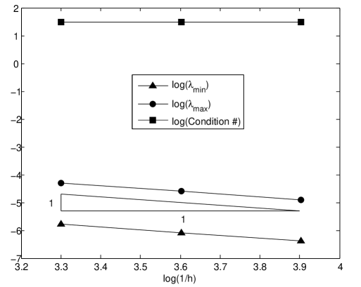
(a) Fixed $\delta$, vary $h$.

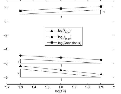
(b) Fixed $h$, vary $\delta$.

Figure 6.1: Condition number for $S_{\Gamma}$ in 1D for (a) fixed $\delta$, allowing $h$ to vary, and (b) fixed $h$, allowing $\delta$ to vary. The condition number of $S_{\Gamma}$ is only weakly $h$-dependent, but varies with $\delta^{-1}$. These figures are plotted from data in Table 6.1. The plots for piecewise linear and piecewise constant shape functions are identical.

$1/h$	$1/\delta$	$\lambda_{\min}$	$\lambda_{\max}$	Condition #
50	10	1.14E-06	1.38E-05	1.21E+01
100	10	2.57E-07	3.48E-06	1.36E+01
200	10	6.61E-08	8.70E-07	1.32E+01

(a) Fixed $\delta$, vary $h$.

$1/h$	$1/\delta$	$\lambda_{\min}$	$\lambda_{\max}$	Condition #
200	10	6.61E-08	8.70E-07	1.32E+01
200	20	7.87E-09	2.18E-07	2.77E+01
200	40	1.09E-09	4.51E-08	4.96E+01

(b) Fixed $h$, vary $\delta$.

Table 6.2: Condition number for $S_{\Gamma}$ in 2D for (a) fixed $\delta$, allowing $h$ to vary, and (b) fixed $h$, allowing $\delta$ to vary. This data is plotted in Figure 6.2.

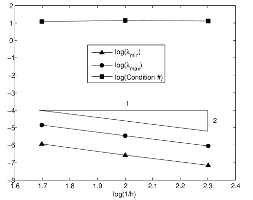
(a) Fixed $\delta$, vary $h$.

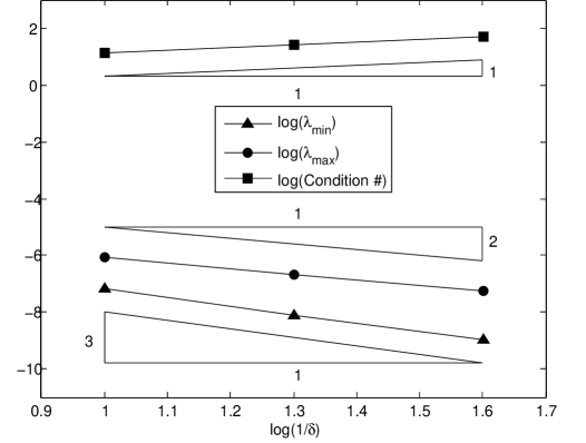
(b) Fixed $h$, vary $\delta$.

Figure 6.2: Condition number for $S_{\Gamma}$ in 2D for (a) fixed $\delta$, allowing $h$ to vary, and (b) fixed $h$, allowing $\delta$ to vary. The condition number of $S_{\Gamma}$ in 2D is only weakly $h$-dependent, but varies with $\delta^{-1}$. These figures are plotted from data in Table 6.2.

6.3 Numerical Verification of the Schur Complement Conditioning

To test the conjecture of the previous section, we discretize the Dirichlet boundary value problem

$$s_{i}(u_{h},v_{h})=(b,v_{h})\qquad\forall v_{h}\in\Lambda_{h},$$ (6.21)

with $u_{h}=0$ on $\mathcal{B}\Omega$, using piecewise constant and piecewise linear shape functions on uniform cartesian mesh, and numerically determine the ratio of the largest and smallest eigenvalues, defining the condition number of the problem.

6.3.1 Results in One Dimension

We define the regions $\Omega_{1}=(0,0.5-\delta/2)$, $\Omega_{2}=(0.5+\delta/2,1)$, and $\Gamma=(0.5-\delta/2,0.5+\delta/2)$, such that $\Gamma$ is always a region of width $\delta$ centered at $x=0.5$. We then compute the largest and smallest eigenvalues of $S_{\Gamma}$. We show results for both piecewise constant and piecewise linear shape functions to verify that the choice of shape function does not play a role in the conditioning of the discrete system.

We first compute the condition number of $S_{\Gamma}$ for different $h$ while holding $\delta$ fixed. Our results appear in Tables 6.1 and Figures 6.1. The minimum and maximum eigenvalues depend linearly on $h$, with a slope of nearly unity. Consequently, the condition number of $S_{\Gamma}$ is only weakly $h$-dependent. We then compute the condition number of $S_{\Gamma}$ for different $\delta$ while holding $h$ fixed, and observe that the condition number varies nearly as $\delta^{-1}$, which is better conditioned than the original stiffness matrix $K$, whose condition number varied with $\delta^{-2}$.

6.3.2 Results in Two Dimensions

We define the regions $\Omega_{1}=(0,0.5-\delta/2)\times(0,1)$, $\Omega_{2}=(0.5+\delta/2,1)\times(0,1)$, and $\Gamma=(0.5-\delta/2,0.5+\delta/2)\times(0,1)$, such that $\Gamma$ is always a region of width $\delta$ centered at $x=0.5$. We then compute the largest and smallest eigenvalues of $S_{\Gamma}$. We consider only piecewise constant shape functions in 2D, having established that the choice of shape function does not affect the conditioning.

We first compute the condition number of $S_{\Gamma}$ for different $h$ while holding $\delta$ fixed, and observe that minimum and maximum eigenvalues depend linearly on $h$ with a slope of approximately two, and again the condition number of $K$ depends only weakly upon the mesh size. Our results appear in Tables 6.2 and Figures 6.2. We then compute the condition number of $S_{\Gamma}$ for different $\delta$ while holding $h$ fixed, and observe that the condition number again varies as $\delta^{-1}$.

7 Conclusions and Future Work

$$\begin{array}[]{ccccccc}\text{{\bf Dim}}&\lambda_{\min}(K)&\lambda_{\max}(K)&\kappa(K)&\lambda_{\min}(S_{\Gamma})&\lambda_{\max}(S_{\Gamma})&\kappa(S_{\Gamma})\\[3.44444pt] \hline\cr\hline\cr\\ \bf{1D}&\mathcal{O}(\delta^{3})&\mathcal{O}(\delta)&\mathcal{O}(\delta^{-2})&\mathcal{O}(\delta^{2})&\mathcal{O}(\delta)&\mathcal{O}(\delta^{-1})\\[3.44444pt] \bf{2D}&\mathcal{O}\left(\delta^{4}\right)&\mathcal{O}(\delta^{2})&\mathcal{O}(\delta^{-2})&\mathcal{O}(\delta^{3})&\mathcal{O}(\delta^{2})&\mathcal{O}(\delta^{-1})\\[3.44444pt] \hline\cr\end{array}$$

Table 7.1: The $\delta$-quantification of the reported numerical results.

We have presented a variational theory for nonlocal problems, such as (1.1). With this theory, we proved the well-posedness of the variational formulation of nonlocal boundary value problems with Dirichlet boundary conditions and practical kernel functions that are relevant to peridynamics. In addition, we proved a spectral equivalence estimate which leads to a mesh-size independent upper bound for the condition number of the stiffness matrix. The spectral equivalence relies on the upper bound (4.21) and the nonlocal Poincaré inequality (4.19) for the lower bound, where in both the $\delta$-dependence and dimension dependence have been explicitly quantified. Supporting numerical experiments demonstrated the sharpness of the upper bound (4.21) as well as the lower bound (4.19). We then constructed a nonlocal domain decomposition framework with associated nonlocal transmission conditions, also proving equivalence between the one-domain and two-domain nonlocal Dirichlet boundary value problems. We defined an energy minimizing extension, analogous to a harmonic extension used in the local case, to analyze the condition number of the nonlocal Schur complement operator. We discretized our two-domain weak form to arrive at a nonlocal Schur complement matrix. Conditioning of the nonlocal Schur complement matrix was explored via numerical studies. We summarize the numerical results in Table 7.1. We observe that $\kappa(K)$ and $\kappa(S_{\Gamma})$ are only weakly dependent upon the mesh size but vary with $\delta^{-2}$ and $\delta^{-1}$, respectively.

It is interesting to compare the conditioning of the discrete nonlocal problem with the conditioning of the (local) discrete Laplace equation. The condition number of the stiffness matrix for the local discrete Laplace equation varies with $h^{-2}$ [17, Theorem B.32], and the corresponding Schur complement matrix condition number varies with $h^{-1}$ [17, Lemma 4.11]. For a fixed mesh size $0<h\ll\delta$, we see from Table 7.1 that the discrete nonlocal stiffness matrix $K$ varies with $\delta^{-2}$, and the condition number of the corresponding nonlocal Schur complement matrix $S_{\Gamma}$ varies as $\delta^{-1}$.

Application of an appropriate preconditioner, involving the solution of a coarse problem, reduces the condition number of the Schur complement of the weak classical (local) Laplace operator from $\mathcal{O}\left((Hh)^{-1}\right)$ to $\mathcal{O}\left((1+\log(H/h))^{2}\right)$, where $H$ is the subdomain size [17, Lemma 4.11], [2, §4.3.6]. One unexplored area involves examining the role of a coarse problem in the nonlocal setting, which has not been considered here. A logical direction would be to expand other substructuring methods to a nonlocal setting, such as Neumann-Dirichlet, Neumann-Neumann, FETI-DP (the dual-primal finite element tearing and interconnecting method) [7], or BDDC (balancing domain decomposition by constraints) [15]. Additional opportunities for future research include addressing convergence analysis for alternative domain decomposition methods not based on substructuring in a nonlocal setting. More fundamental concepts in Schwarz theory such as stable decompositions and local solvers need to be reconstructed for nonlocal problems to support convergence analysis for additive, multiplicative, and hybrid algorithms.

References

- [1] J. S. Przemieniecki, Matrix structural analysis of substructures, AIAA Journal 1 (1) (1963) 138–147.
- [2] B. Smith, P. E. Bjørstad, W. Gropp, Domain Decomposition: Parallel Multilevel Methods for Elliptic Partial Differential Equations, Cambridge University Press, 1999.
- [3] C. Farhat, F.-X. Roux, A method of finite element tearing and interconnecting and its parallel solution algorithm, Internat. J. Numer. Meths. Engrg. 32 (1991) 1205–1227.
- [4] C. Farhat, F.-X. Roux, Implicit parallel processing in structural mechanics, in: J. T. Oden (Ed.), Computational Mechanics Advances, Vol. 2 (1), North-Holland, 1994, pp. 1–124.
- [5] C. Farhat, K. H. Pierson, M. Lesoinne, The second generation of FETI methods and their application to the parallel solution of large-scale linear and geometrically nonlinear structural analysis problems, Computer Methods in Applied Mechanics and Engineering 184 (2000) 333–374.
- [6] D. Rixen, C. Farhat, A simple and efficient extension of a class of substructure based preconditioners to heterogeneous structural mechanics problems, Inter. J. Numer. Meth. Engrg. 44 (1999) 489–516.
- [7] P. L. K. Pierson C. Farhat, M. Lesoinne, D. Rixen, FETI-DP: A Dual-Primal unified FETI method - part I: A faster alternative to the two-level FETI method, Int. J. Numer. Numer. Engng. 50 (2001) 1523–1544.
- [8] J. H. Bramble, J. E. Pasciak, A. H. Schatz, The construction of preconditioners for elliptic problems by substructuring I, Math. Comp. 47 (1986) 103–134.
- [9] J. H. Bramble, J. E. Pasciak, A. H. Schatz, The construction of preconditioners for elliptic problems by substructuring II, Math. Comp. 49 (1987) 1–16.
- [10] J. H. Bramble, J. E. Pasciak, A. H. Schatz, The construction of preconditioners for elliptic problems by substructuring III, Math. Comp. 51 (1988) 141–430.
- [11] J. H. Bramble, J. E. Pasciak, A. H. Schatz, The construction of preconditioners for elliptic problems by substructuring IV, Math. Comp. 53 (1989) 1–24.
- [12] C. Farhat, J. Mandel, F.-X. Roux, Optimal convergence properties of the FETI domain decomposition method, Comput. Methods Appl. Mech. Engrg. 115 (1994) 367–388.
- [13] J. Mandel, Balancing domain decomposition, Comm. Numer. Methods Engrg. 9 (1993) 233–241.
- [14] A. Klawonn, O. B. Widlund, FETI and Neumann -Neumann iterative substructuring methods: connections and new results, Comm. Pure Appl. Math. 54 (2001) 57–90.
- [15] C. R. Dohrmann, A preconditioner for substructuring based on constrained energy minimization, SIAM J. Sci. Comput. 25 (2003) 246–258.
- [16] A. Quarteroni, A. Valli, Domain Decomposition Methods for Partial Differential Equations, Oxford University Press, Oxford, 1999.
- [17] A. Toselli, O. Widlund, Domain Decomposition Methods – Algorithms and Theory, Springer Series in Computational Mathematics, Springer, 2005.
- [18] J. H. Cushman, T. R. Glinn, Nonlocal dispersion in media with continuously evolving scales of heterogeneity, Trans. Porous Media 13 (1993) 123–138.
- [19] G. Dagan, The significance of heterogeneity of evolving scales to transport in porous formations, Water Resour. Res. 30 (1994) 3327–3336.
- [20] R. K. Sinha, R. E. Ewing, R. D. Lazarov, Some new error estimates of a semidiscrete finite volume element method for a parabolic integro-differential equation with nonsmooth initial data, SIAM J. Numer. Anal. 43 (6) (2006) 2320–2344.
- [21] O. G. Bakunin, Turbulence and Diffusion: Scaling Versus Equations, Springer Series in Synergetics, Springer, 2008.
- [22] A. C. Eringen, Nonlocal Continuum Field Theories, Springer, New York, 2002.
- [23] P. Seleson, M. L. Parks, M. Gunzburger, R. B. Lehoucq, Peridynamics as an upscaling of molecular dynamics, Multiscale Modeling and Simulation 8 (1) (2009) 204–227.
- [24] B. Alali, R. Lipton, Multiscale analysis of heterogeneous media in in the peridynamic formulation, IMA Preprint Series 2241, Institute for Mathematics and its Applications, University of Minnesota (February 2009).
- [25] M. Gunzburger, R. B. Lehoucq, A nonlocal vector calculus with application to nonlocal boundary value problems, Multiscale Model. Simul. 8 (5) (2010) 1581–1598.
- [26] F. Andreu, J. M. Mazon, J. D. Rossi, J. Toledo, The Neumann problem for nonlocal nonlinear diffusion equations, J. Evol. Eqn. 8 (2008) 189–215.
- [27] F. Andreu, J. M. Mazon, J. D. Rossi, J. Toledo, A nonlocal p-Laplacian evolution equation with Neumann boundary conditions, J. Math. Pures Appl. 90 (2008) 201–227.
- [28] F. Andreu, J. M. Mazon, J. D. Rossi, J. Toledo, A nonlocal p-Laplacian evolution equation with nonhomogeneous Dirichlet boundary conditions, SIAM J. Math. Anal. 40 (5) (2009) 1815–1851.
- [29] L. Caffarelli, L. Silvestre, An extension problem related to the fractional Laplacian, Comm. Partial Differential Equations 32 (2007) 1245–1260.
- [30] L. Caffarelli, L. Silvestre, Regularity theory for fully nonlinear integro-differential equations, Comm. Pure Appl. Math. 62 (2009) 597–638.
- [31] L. Silvestre, Hölder estimates for solutions of integro differential equations like the fractional Laplace, Indiana Univ. Math. J. 55 (2006) 1155–1174.
- [32] Q. Du, K. Zhou, Mathematical analysis for the peridynamic nonlocal continuum theory, Mathematical Modelling and Numerical Analysis, doi:10.1051/m2an/2010040 (2010).
- [33] K. Zhou, Q. Du, Mathematical and numerical analysis of linear peridynamic models with nonlocal boundary conditions, SIAM J. Num. Anal. 48 (5) (2010) 1759–1780.
- [34] C. Carrillo, P. Fife, Spatial effects in discrete generation population models, J. Math. Biol. 50 (2) (2005) 161–188.
- [35] G. Gilboa, S. Osher, Nonlocal operators with applications to image processing, Multiscale Modeling and Simulation 7 (3) (2008) 1005–1028.
- [36] N. Birch, R. Lehoucq, Classical, nonlocal, and fractional diffusion equations, Tech. Rep. SAND 2010-1762J, Sandia National Laboratories (2010).
- [37] P. Fife, Some nonclassical trends in parabolic and parabolic-like evolutions, in: Trends in nonlinear analysis, Springer, 2003, pp. 153–191.
- [38] S. A. Silling, Reformulation of elasticity theory for discontinuities and long-range forces, J. Mech. Phys. Solids 48 (2000) 175–209.
- [39] S. A. Silling, E. Askari, A meshfree method based on the peridynamic model of solid mechanics, Computers and Structures 83 (2005) 1526–1535.
- [40] S. Silling, M. Epton, O. Weckner, J. Xu, E. Askari, Peridynamic states and constitutive modeling, J. Elasticity 88 (2007) 151–184.
- [41] E. Emmrich, O. Weckner, The peridynamic equation and its spatial discretization, Mathematical Modelling and Analysis 12 (1) (2007) 17–27.
- [42] B. Aksoylu, T. Mengesha, Results on nonlocal boundary value problems, Numerical Functional Analysis and Optimization 31 (12) (2010) 1301–1317.
- [43] E. Emmrich, O. Weckner, On the well-posedness of the linear peridynamic model and its convergence towards the Navier equation of linear elasticity, Commun. Math. Sci. 5 (4) (2007) 851–864.
- [44] S. A. Silling, R. B. Lehoucq, Convergence of peridynamics to classical elasticity theory, J. Elasticity 93 (2008) 13–37.