Quasi-Fuchsian Surfaces In Hyperbolic Link Complements

Joseph D. Masters and Xingru Zhang

Abstract. We show that every hyperbolic link complement contains closed quasi-Fuchsian surfaces. As a consequence, we obtain the result that on a hyperbolic link complement, if we remove from each cusp of the manifold a certain finite set of slopes, then all remaining Dehn fillings on the link complement yield manifolds with closed immersed incompressible surfaces.

1 Introduction

By a link complement we mean, in this paper, the complement of a link in a closed connected orientable $3$-manifold. A link complement is said to be hyperbolic if it admits a complete hyperbolic metric of finite volume. By a surface we mean, in this paper, the complement of a finite (possibly empty) set of points in the interior of a compact, orientable $2$-manifold (which may not be connected). By a surface in a $3$-manifold $W$, we mean a continuous, proper map $f:S{\rightarrow}W$ from a surface $S$ into $W$. A surface $f:S{\rightarrow}W$ in a 3-manifold $W$ is said to be connected if and only if $S$ is connected. A surface $f:S{\rightarrow}W$ in a 3-manifold $W$ is said to be incompressible if each component $S_{j}$ of $S$ is not a $2$-sphere and the induced homomorphism $f^{*}:\pi_{1}(S_{j},s){\rightarrow}\pi_{1}(W,f(s))$ is injective for any choice of base point $s$ in $S_{j}$. A surface $f:S{\rightarrow}W$ in a 3-manifold $W$ is said to be essential if it is incompressible and for each component $S_{j}$ of $S$, the map $f:S_{j}{\rightarrow}W$ cannot be properly homotoped into a boundary component or an end component of $W$.

Connected essential surfaces in hyperbolic link complements can be divided into three mutually exclusive geometric types: quasi-Fuchsian surfaces, geometrically infinite surfaces, and essential surfaces with accidental parabolics. Geometrically these three types of surfaces can be characterized by their limit sets as follows: a connected essential surface $f:S{\rightarrow}M$ in a hyperbolic link complement $M$ is Quasi-Fuchsian if and only if the limit set of the subgroup $f^{*}(\pi_{1}(S))\subset\pi_{1}(M)$ is a Jordon circle in the boundary $2$-sphere of the hyperbolic $3$-space $\mathbb{H}^{3}$; is geometrically infinite if and only if the limit set of $f^{*}(\pi_{1}(S))$ is the whole $2$-sphere; and is having accidental parabolics otherwise. Topologically these three types of surfaces can be characterized as follows: a connected essential surface $f:S{\rightarrow}M$ in a hyperbolic link complement $M$ is geometrically infinite if and only if it can be lifted (up to homotopy) to a fiber in some finite cover of $M$; is having accidental parabolics if and only $S$ contains a closed curve which cannot be freely homotoped in $S$ into a cusp of $S$ but can be freely homotoped in $M$ into a cusp of $M$, and is quasi-Fuchsian otherwise.

In [MZ] it was shown that every hyperbolic knot complement contains closed quasi-Fuchsian surfaces. In this paper we extend this result to hyperbolic link complements.

Theorem 1.1.

Every hyperbolic link complement contains closed quasi-Fuchsian surfaces.

This yields directly the following consequence.

Corollary 1.2.

For every given hyperbolic link complement $M$, if we remove certain finitely many slopes from each cusp of $M$, then all remaining Dehn fillings produce manifolds which contain closed incompressible surfaces.

We note that Corollary 1.2 would also be a consequence of Khan and Markovic’s recent claim that every closed hyperbolic 3-manifold contains a surface subgroup.

This paper is an extension of [MZ] where the existence of closed quasi-Fuchsian surfaces in any hyperbolic knot complement was proved. The proof of Theorem 1.1 follows essentially the approach given in [MZ]. To avoid repetition, we shall assume the reader is familiar with the machinery laid out in [MZ]. In particular we shall use most of the terms and properties about hyperbolic $3$-manifolds and about groups established in [MZ], without recalling them in detail, and shall omit details of constructions and proof of assertions whenever they are natural generalization of counterparts of [MZ].

To help the reader to get a general idea about which parts of our early arguments are needed to be adjusted nontrivially, we first very briefly recall how a closed quasi-Fuchsian surface was constructed in a hyperbolic knot complement. We started with a pair of connected bounded embedded quasi-Fuchsian surfaces in a given hyperbolic knot exterior $M^{-}$ (which is truncation of a hyperbolic knot complement $M$) with distinct boundary slopes in ${\partial}M^{-}$. We then considered two hyperbolic convex $I$-bundles resulting from the two corresponding quasi-Fuchsian surface groups. By a careful “convex gluing” of two suitable finite covers of some truncated versions of the two $I$-bundles, and then “capping off convexly” by a solid cusp, we constructed a convex hyperbolic $3$-manifold $Y$ with a local isometry $f$ into the given hyperbolic knot complement $M$. The manifold $Y$ had non-empty boundary each component of which provided a closed quasi-Fuchsian surface in $M$ under the map $f$. To find the required finite covers of the truncated $I$-bundles and at the same time to lift certain immersions to embeddings, we needed a stronger version of subgroup separability property for surface groups with boundary, which was proved using Stallings’ folding graph techniques.

Now to extend the construction to work for hyperbolic link complements, we first need to prove, for any given hyperbolic link exterior $M^{-}$, the existence of two properly embedded bounded quasi-Fuchsian surfaces $S_{i}^{-}$, $i=1,2$, in $M^{-}$, each of which is not necessarily connected, with the crucial property that for each of $i=1,2$ and each component $T_{j}$ of ${\partial}M^{-}$, $S_{i}^{-}\cap T_{j}$ is a non-empty set of simple closed essential curves, and furthermore the slope of the curves $S_{1}^{-}\cap T_{j}$ is different from that of $S_{2}^{-}\cap T_{j}$ for each $T_{j}$. The proof of this result, given in Section 2, is based on work of Culler-Shalen [CS] and Cooper-Long [CL] and Thurston [T], making use of the $SL_{2}({\mathbb{C}})$ character variety of the link exterior $M^{-}$ and some special properties of essential surfaces in hyperbolic $3$-manifolds with accidental parabolics. With the given two surfaces $S_{i}^{-}$, $i=1,2$, we may construct two corresponding convex $I$-bundles (in the current situation each $I$-bundle may not be connected). Following the approach in [MZ] we still want to choose a suitable cover for each component of each of the truncated $I$-bundles, and “convexly glue” them all together in certain way and “convexly cap off” with $m$ (which is the number of components of ${\partial}M^{-}$) solid cusps, to form a convex hyperbolic $3$-manifold $Y$, with a local isometry $f$ into $M$, such that the boundary of $Y$ is a non-empty set, each component of which is mapped by $f$ to a closed quasi-Fuchsian surface in $M$.

As before, we want to choose the cover so that the boundary components of $S_{i}^{-}$ unwrap as much as possible. And if the two surfaces $S_{i}^{-}$ are connected, our previous arguments go through with very little change. However, if the surfaces $S_{i}^{-}$ are disconnected, complications arise. In order to piece the different covers together, we need to know that they all have the same degree. And this turns out to require a non-trivial strengthening of our previous separability result; see Theorem 5.1. The proof of this property uses a careful refinement of the folding graph arguments used in [MZ].

2 Cusped qausi-Fuchsian surfaces in hyperbolic link complements

From now on let $M$ be a given hyperbolic link complement of $m\geq 2$ cusps. For each of $i=1,...,m$, let $C_{i}$ be a fixed $i$-th cusp of $M$ which is geometric, embedded and small enough so that $C_{1},...,C_{m}$ are mutually disjoint. The complement of the interior of $C_{1}\cup...\cup C_{m}$ in $M$, which we denote by $M^{-}$, is a compact, connected and orientable $3$-manifold whose boundary is a set of $m$ tori. We call $M^{-}$ a truncation of $M$. Let $T_{k}={\partial}C_{k}$, $k=1,...,m$. Then ${\partial}M^{-}=T_{1}\cup...\cup T_{m}$.

Lemma 2.1.

There are two embedded essential quasi-Fuchsian surfaces $S_{1}$ and $S_{2}$ in $M$ (each $S_{i}$ may not be connected) such that for each of $i=1,2$ and each of $k=1,...,m$, $S_{i}\cap T_{k}$ is a nonempty set of parallel simple closed essential curves in $T_{k}$ of slope $\lambda_{i,k}$ and $\lambda_{1,k}\neq\lambda_{2,k}$.

Proof.  It is equivalent to show that the truncation $M^{-}$ of $M$ contains two properly embedded bounded essential surfaces $S_{1}^{-}$ and $S_{2}^{-}$ such that:
(i) For each of $i=1,2$, each component of $S_{i}^{-}$ is not a fiber or semi-fiber of $M^{-}$.
(ii) For each of $i=1,2$, any closed curve in $S_{i}^{-}$ that can be freely homotoped in $M^{-}$ into ${\partial}M^{-}$ can also be freely homotoped in $S_{i}^{-}$ into ${\partial}S_{i}^{-}$.
(iii) For each of $i=1,2$ and each of $k=1,...,m$, $S_{i}^{-}$ has non-empty boundary on $T_{k}$ of boundary slope $\lambda_{i,k}$ and $\lambda_{1,k}\neq\lambda_{2,k}$.

Let $\{\gamma_{k}\subset T_{k};k=1,...,m\}$ be any given set of $n$ slopes. By [CS, Theorem 3], there is a properly embedded essential surface $S_{1}^{-}$ (maybe disconnected) in $M^{-}$ with the following properties (in fact the surface $S_{1}^{-}$ is obtained through a nontrivial group action on a simplicial tree associated to an ideal point of a curve in a component of the $SL(2,{\mathbb{C}})$-character variety of $M^{-}$ which contains the character of a discrete faithful representation of $\pi_{1}(M^{-})$):

(1) No component of $S_{1}^{-}$ is a fiber or semi-fiber of $M^{-}$.

(2) For each of $k=1,...,m$, $S_{1}^{-}$ has non-empty boundary on $T_{k}$ of boundary slope $\lambda_{1,k}$ which is different from $\gamma_{k}$.

(3) If an element of $\pi_{1}(M^{-})$ is freely homotopic to a curve in $M^{-}\setminus S_{1}^{-}$, then it is contained in a vertex stabilizer of the action on the tree.

(4) If an element of $\pi_{1}(M^{-})$ is freely homotopic to $\gamma_{k}$, then it is not contained in any vertex stabilizer of the action on the tree and thus must intersect $S_{1}^{-}$.

(5) If an element of $\pi_{1}(M^{-})$ is freely homotopic to a curve in $S_{1}^{-}$, then it is contained in an edge stabilizer of the tree.
It follows that

(6) If an element of $\pi_{1}(M^{-})$ is freely homotopic to a simple closed essential curve in $T_{k}$ whose slope is different from $\lambda_{1,k}$, then it is not contained in any vertex stabilizer of the action on the tree.

Let $S^{-}_{1,j}$, $j=1,...,n_{1}$, be the components of $S^{-}_{1}$. If some $S^{-}_{1,j}$ has a closed curve which cannot be freely homotoped in $S_{1}^{-}$ into ${\partial}S_{1}^{-}$ but can be freely homotoped in $M^{-}$ into ${\partial}M$, then arguing as in [CL, Lemma 2.1], we see that there is an embedded annulus $A$ in $M^{-}\setminus S^{-}_{1,j}$ such that one boundary component, denoted $a_{1}$, of $A$ lies in $S_{1,j}^{-}$ and is not boundary parallel in $S^{-}_{1,j}$, and the other boundary component, denoted $a_{2}$, of $A$ is contained in some boundary component $T_{k}$ of $M^{-}$. By Properties (5) and (6) listed above, we have

(7) $a_{2}\subset T_{k}$ must have the slope $\lambda_{1,k}$.

Now consider in $A$ the intersection set $A\cap(S^{-}_{1}-S^{-}_{1,j})$ of $A$ with other components of $S_{1}^{-}$. By Property (7), we may assume that ${\partial}A\cap(S^{-}_{1}-S^{-}_{1,j})=\emptyset$. Thus by proper isotopy of $(S_{1}^{-}-S^{-}_{1,j},{\partial}(S^{-}_{1}-S^{-}_{1,j}))\subset(M^{-},{\partial}M^{-})$ and surgery (if necessary) we may assume that each component of $A\cap(S^{-}_{1}-S^{-}_{1,j})$ is a circle which is isotopic in $A$ to the center circle of $A$ and if the component is contained in $S^{-}_{1,j^{\prime}}$, then it is not boundary parallel in $S^{-}_{1,j^{\prime}}$. So the component of $A\cap(S^{-}_{1}-S^{-}_{1,j})$, denoted $a_{1}^{\prime}$, which is closest to $a_{2}$ in $A$, cuts out from $A$ an sub-annulus $A^{\prime}$ which is properly embedded in $M^{-}\setminus S^{-}_{1}$ such that $a_{1}^{\prime}$ lies in $S^{-}_{1,j^{\prime}}$, for some $j^{\prime}$, and is not boundary parallel in $S^{-}_{1,j^{\prime}}$. So we may perform the annulus compression on $S^{-}_{1,j^{\prime}}$ along $A^{\prime}$ to get an essential surface which still satisfies the properties (1)-(6) above (because the new resulting surface can be considered as a subsurface of the old surface $S_{1}^{-}$ and because of property (7)) but has larger Euler characteristic. Thus such annulus compression must terminate in a finite number of times. So eventually we end up with a surface, which we still denote by $S_{1}^{-}$, satisfying the condition

(8) Any closed curve in $S_{1}^{-}$ that can be freely homotoped in $M^{-}$ into ${\partial}M$ can be freely homotoped in $S_{1}^{-}$ into ${\partial}S_{1}^{-}$.

Now letting $\gamma_{k}=\lambda_{1,k},k=1,...,m$, and repeating the above arguments, we may get another properly embedded essential surface $S_{2}^{-}$ such that

(1’) Each component of $S_{2}^{-}$ is not a fiber or semi-fiber of $M^{-}$.

(2’) For each of $k=1,...,m$, $S_{2}^{-}$ has non-empty boundary on $T_{k}$ of boundary slope $\lambda_{2,k}$ which is different from $\lambda_{1,k}$.

(8’) Any closed curve in $S_{2}^{-}$ that can be freely homotoped in $M^{-}$ into ${\partial}M$ can be freely homotoped in $S_{2}^{-}$ into ${\partial}S_{2}^{-}$.

So $S_{1}^{-}$ and $S_{2}^{-}$ satisfy conditions (i), (ii) and (iii) listed above. The lemma is thus proved.   $\diamondsuit$

Let $S_{i},i=1,2$ be the two surfaces provided by Lemma 2.1. By taking disjoint parallel copies of some components of $S_{i}$ (if necessary), we may and shall assume

Condition 2.2.

For each $i=1,2$ and $k=1,...,m$, $S_{i}\cap T_{k}$ has a positive, even number of components.

Notation 2.3.

Let $S_{i,j}$, $j=1,...,n_{i}$, be components of $S_{i}$, $i=1,2$. Let $i_{*}$ be the number such that $\{i,i_{*}\}=\{1,2\}$ for $i=1,2$. Let $S_{i}^{-}=S_{i}\cap M^{-}$ and let ${\partial}_{k}S_{i,j}^{-}$ be the boundary components of $S^{-}_{i,j}$ on $T_{k}$ (which may be empty for some $j$’s) and let ${\partial}_{k}S_{i}^{-}=\cup_{j}{\partial}_{k}S_{i,j}^{-}$. Now for each $i=1,2,k=1,...,m$, let $d_{i,k}$ be the geometric intersection number in $T_{k}$ between a component of ${\partial}_{k}S_{i}^{-}$ and the whole set ${\partial}_{k}S_{i_{*}}$. Obviously $d_{i,k}$ is independent of the choice of the component of ${\partial}_{k}S_{i}^{-}$. By Condition 2.2, $d_{i,k}\geq 2$ is even for each $i,k$. Now set

$$d_{i}=lcm\{d_{i,k};\;k=1,...,m\},$$

the (positive) least common multiple. Then $d_{i}\geq 2$ is even for each $i=1,2$.

Let $\mathbb{H}^{3}$ be the hyperbolic $3$-space in the upper half space model, let $S_{\infty}^{2}$ be the $2$-sphere at $\infty$ of $\mathbb{H}^{3}$ and let $\overline{\mathbb{H}}^{3}=\mathbb{H}^{3}\cup S_{\infty}^{2}$.

By Mostow-Prasad rigidity, the fundamental group of $M$ (for any fixed choice of base point) can be uniquely identified as a discrete torsion free subgroup ${\Gamma}$ of $Isom^{+}(\mathbb{H}^{3})$ up to conjugation in $Isom(\mathbb{H}^{3})$ so that $M=\mathbb{H}^{3}/{\Gamma}$. We shall fix one such identification. Let $p:\mathbb{H}^{3}{\rightarrow}M$ be the corresponding covering map.

For the given surface $S_{i,j}$ in $M$ (for each $i,j$), we identify its fundamental group with a quasi-Fuchsian subgroup ${\Gamma}_{i,j}$ of ${\Gamma}$ as follows. As $S_{i,j}$ is embedded in $M$ we may consider it as a submanifold of $M$. Fix a component $\tilde{S}_{i,j}$ of $p^{-1}(S_{i,j})$ (topologically $\tilde{S}_{i,j}$ is an open disk in $\mathbb{H}^{3}$), there is a subgroup ${\Gamma}_{i,j}$ in the stabilizer of $\tilde{S}_{i,j}$ in ${\Gamma}$ such that $S_{i,j}=\tilde{S}_{i,j}/{\Gamma}_{i,j}$.

Note that the limit set $\Lambda_{i,j}$ of ${\Gamma}_{i,j}$ is a Jordan circle in the $2$-sphere $S^{2}_{\infty}$ at the $\infty$ of $\mathbb{H}^{3}$. Let $H_{i,j}$ be the convex hull of $\Lambda_{i,j}$ in $\mathbb{H}^{3}$.

Let ${\cal B}_{k}=p^{-1}(C_{k})$, $k=1,...,m$, and ${\cal B}=p^{-1}(C)$. Then by our assumption on $C$, ${\cal B}$ is a set of mutually disjoint horoballs in $\mathbb{H}^{3}$. Let $B$ be a component of ${\cal B}$ and let ${\partial}B$ be the frontier of $B$ in $\mathbb{H}^{3}$. Then ${\partial}B$ with the induced metric is isometric to a Euclidean plane. We shall simply call ${\partial}B$ a Euclidean plane. A strip between two parallel Euclidean lines in ${\partial}B$ will be called a Euclidean strip in ${\partial}B$. Note that every Euclidean line in ${\partial}B$ bounds a totally geodesic half plane in $B$ (which is perpendicular to ${\partial}B$). By a $3$-dimensional strip region in $B$ we mean a region in $B$ between two totally geodesic half planes in $B$ bounded by two parallel disjoint Euclidean lines in ${\partial}B$.

Lemma 2.4.

If the cusp set $C=C_{1}\cup...\cup C_{m}$ of $M$ is small enough, then for each component $B$ of ${\cal B}$ whose point at $\infty$ is a parabolic fixed point of ${\Gamma}_{i,j}$, $H_{i,j}\cap B$ is a $3$-dimensional strip region in $B$.

Proof.  The proof is similar to that of [MZ, Lemma 5.2].   $\diamondsuit$

From now on we assume that $C$ has been chosen so that Lemma 2.4 holds for all $i=1,2,j=1,...,n_{i}$. For a fixed small $\epsilon>0$, let $X_{i,j}$ be the $\epsilon$-collared neighborhood of $H_{i,j}$ in $\mathbb{H}^{3}$. Then it follows from Lemma 2.4 that for each component $B$ of ${\cal B}$ whose point at $\infty$ is a parabolic fixed point of ${\Gamma}_{i,j}$,, $X_{i,j}\cap B$ is a $3$-dimensional strip region in $B$, for all $i=1,2,j=1,...,n_{i}$, by geometrically shrinking $C$ further if necessary.

Note that $X_{i,j}$ is a metrically complete and strictly convex hyperbolic $3$-submanifold of $\mathbb{H}^{3}$ with $C^{1}$ boundary, invariant under the action of ${\Gamma}_{i,j}$. Let

$${\cal B}_{i,j}=\{X_{i,j}\cap B;\mbox{$B$ a component of ${\cal B}$ based at a parabolic fixed point of ${\Gamma}_{i,j}$}\}.$$

We call ${\cal B}_{i,j}$ the horoball region of $X_{i,j}$. Let $X_{i,j}^{-}=X_{i,j}\setminus{\cal B}_{i,j}$, and call $X_{i,j}^{-}\cap{\partial}{\cal B}_{i,j}$ the parabolic boundary of $X_{i,j}^{-}$, denoted by ${\partial}_{p}X_{i,j}^{-}$. Note that $X_{i,j}^{-}$ is locally convex everywhere except on its parabolic boundary.

Each of $X_{i,j}$, ${\cal B}_{i,j}$, $X_{i,j}^{-}$ and ${\partial}_{p}X_{i,j}^{-}$ is invariant under the action of ${\Gamma}_{i,j}$. Let $Y_{i,j}=X_{i,j}/{\Gamma}_{i,j}$, which is a metrically complete and strictly convex hyperbolic $3$-manifold with boundary. Topologically $Y_{i,j}=S_{i,j}\times I$, where $I=[-1,1]$. There is a local isometry $f_{i,j}$ of $Y_{i,j}$ into $M$, which is induced from the covering map $\mathbb{H}^{3}/{\Gamma}_{i,j}\;\longrightarrow\;M$ by restriction on $Y_{i,j}$, since $Y_{i,j}=X_{i,j}/{\Gamma}_{i,j}$ is a submanifold of $\mathbb{H}^{3}/{\Gamma}_{i,j}$. Also $p|_{X_{i,j}}=f_{i,j}\circ p_{i,j}$, where $p_{i,j}$ is the universal covering map $X_{i,j}{\rightarrow}Y_{i,j}=X_{i,j}/{\Gamma}_{i,j}$. Let $Y_{i,j}^{-}=X_{i,j}^{-}/{\Gamma}_{i,j}$, let ${\cal C}_{i,j}={\cal B}_{i,j}/{\Gamma}_{i,j}$, and let ${\partial}_{p}Y_{i,j}^{-}={\partial}_{p}X_{i,j}^{-}/{\Gamma}_{i,j}$. We call ${\cal C}_{i,j}$ the cusp part of $Y_{i,j}$, and call ${\partial}_{p}Y_{i,j}^{-}$ the parabolic boundary of $Y_{i,j}^{-}$, which is the frontier of $Y_{i,j}^{-}$ in $Y_{i,j}$ and is also the frontier of ${\cal C}_{i,j}$ in $Y_{i,j}$. Each component of ${\partial}_{p}Y_{i,j}^{-}$ is a Euclidean annulus. The manifold $Y_{i,j}^{-}$ is locally convex everywhere except on its parabolic boundary. Topologically $Y_{i,j}^{-}=S_{i,j}^{-}\times I$.

As in [MZ, Section 5], we fix a product $I$-bundle structure for $Y_{i,j}=S_{i,j}\times I$ such that each component of ${\cal C}_{i,j}$ has the induced $I$-bundle structure which is the product of a totally geodesic cusp annulus and the $I$-fiber (i.e. we assume that $(S_{i,j}\times\{0\})\cap{\cal C}_{i,j}$ is a set of totally geodesic cusp annuli). We let every free cover of $Y_{i,j}$ have the induced $I$-bundle structure. In particular $X_{i,j}$ has the induced $I$-bundle structure from that of $Y_{i,j}$, and this structure is preserved by the action of ${\Gamma}_{i,j}$; i.e. every element of ${\Gamma}_{i,j}$ sends an $I$-fiber of $X_{i,j}$ to an $I$-fiber of $X_{i,j}$. Similar to [MZ, Corollary 5.6], we have

Lemma 2.5.

For each of $i=1,2,j=1,...,n_{i}$, there is an upper bound for the lengths of the $I$-fibers of $X_{i,j}$.   $\diamondsuit$

The restriction of the map $f_{i,j}$ on the center surface $S_{i,j}\times\{0\}$ of $Y_{i,j}=S_{i,j}\times I$ may not be an embedding in general but by Lemma 2.4 we may and shall assume that the map is an embedding when restricted on $(S_{i,j}\times\{0\})\cap{\cal C}_{i,j}$. We now replace our original embedded surface $S_{i,j}$ by the center surface $f_{i,j}:S_{i,j}\times\{0\}$ and we simply denote $S_{i,j}\times\{0\}$ by $S_{i,j}$.

The restriction map $f_{i,j}:(Y_{i,j}^{-},{\partial}_{p}Y_{i,j}^{-}){\rightarrow}(M^{-},{\partial}M^{-})$ is a proper map of pairs and $f_{i,j}:(S_{i,j}^{-},{\partial}S_{i,j}^{-}){\rightarrow}(M^{-},{\partial}M^{-})$ is a proper map which is an embedding on ${\partial}S_{i,j}^{-}$ (This property will remain valid if we shrink the cusp $C$ of $M$ geometrically). In fact $f_{i,j}({\partial}S_{i,j}^{-})$ are embedded Euclidean circles in ${\partial}M^{-}$. Hence boundary slopes of the new quasi-Fuchsian surfaces $f_{i,j}:(S_{i,j}^{-},{\partial}S_{i,j}^{-}){\rightarrow}(M^{-},{\partial}M^{-})$ are defined and are the same as those of the original embedded surfaces $S_{i,j}^{-}$.

Note 2.6.

As $f_{i,j}:{\partial}S_{i,j}^{-}{\rightarrow}{\partial}M^{-}$ is an embedding, we sometimes simply consider ${\partial}S_{i,j}^{-}$ as subset of ${\partial}M^{-}$, for each $i=1,2,j=1,...,n_{i}$. By choosing a slightly different center surface for $Y_{i,j}$ (if necessary), we may assume that the components of $\{{\partial}S_{i,j}^{-},j=1,...,n_{i}\}$ are mutually disjoint in ${\partial}M^{-}$, for each fixed $i=1,2$. So the numbers $d_{i,k}$, $d_{i}$ defined in Notation 2.3 remain well defined for the current surface $f_{i,j}:(S_{i,j}^{-},{\partial}S_{i,j}^{-}){\rightarrow}(M,{\partial}M)$ and are the same numbers as given there, for all $i,j$. Also ${\partial}_{k}S_{i,j}^{-}$ remain defined as before for all $i,j$.

Let $\tilde{S}_{i,j}$ and $\tilde{S}_{i,j}^{-}$ be the corresponding center surfaces of $X_{i,j}$ and $X_{i,j}^{-}$ respectively.

Note also that if a component of ${\partial}S_{i,j}^{-}$ intersects a component of ${\partial}S_{i_{*},j^{\prime}}^{-}$ in some component $T_{k}$ of ${\partial}M^{-}$, then they intersect geometrically in $T_{k}$, and their intersection points in $T_{k}$ are one-to-one corresponding to the geodesic rays of $f_{i,j}(S_{i,j})\cap f_{i_{*},j^{\prime}}(S_{i_{*},j^{\prime}})\cap C_{k}$.

We fix an orientation for $S_{i,j}$, and let $S_{i,j}^{-}$ and ${\partial}S_{i,j}^{-}$ have the induced orientation.

3 Construction of intersection pieces $K_{i,j}$

Suppose that ${\partial}S_{i,j}^{-}$ intersects ${\partial}S_{i_{*},j^{\prime}}^{-}$ for some $j,j^{\prime}$. We construct the “intersection pieces” $K_{i,j,j^{\prime}}$ and $K_{i_{*},j^{\prime},j}$ between $Y_{i,j}$ and $Y_{i_{*},j^{\prime}}$ in a similar fashion as in [MZ, Section 6] such that
(1) $K_{i,j,j^{\prime}}$ and $K_{i_{*},j^{\prime},j}$ are isometric.
(2) Each component of $K_{i,j,j^{\prime}}$ or of $K_{i_{*},j^{\prime},j}$ is a metrically complete convex hyperbolic $3$-manifold.
(3) There are local isometries $g_{i,j,j^{\prime}}:K_{i,j,j^{\prime}}{\rightarrow}Y_{i,j}$ and $g_{i_{*},j^{\prime},j}:K_{i_{*},j^{\prime},j}{\rightarrow}Y_{i_{*},j^{\prime}}$.
(4) $K^{-}_{i,j,j^{\prime}}$ and $K^{-}_{i_{*},j^{\prime},j}$ (which are the truncated versions of $K_{i,j,j^{\prime}}$ and $K_{i_{*},j^{\prime},j}$ respectively) are compact.
(5) Each component of the parabolic boundary ${\partial}_{p}K_{i,j,j^{\prime}}^{-}$ of $K_{i,j,j^{\prime}}^{-}$ is a Euclidean parallelogram, the number of cusp ends of $K_{i,j,j^{\prime}}$ is precisely the number of intersection points between $f_{i,j}({\partial}S_{i,j}^{-})$ and $f_{i_{*},j^{\prime}}({\partial}S_{i_{*},j^{\prime}}^{-})$. Similar properties hold for $K_{i_{*},j^{\prime},j}$.
(6) The restriction of $g_{i,j,j^{\prime}}$ to $K_{i,j,j^{\prime}}\setminus K_{i,j,j^{\prime}}^{-}$ is an embedding and so is the restriction of $g_{i_{*},j^{\prime},j}$ to $K_{i_{*},j^{\prime},j}\setminus K_{i_{*},j^{\prime},j}^{-}$.
(7) $f_{i,j}(g_{i,j,j^{\prime}}(K_{i,j,j^{\prime}}\setminus K_{i,j,j^{\prime}}^{-}))$ contains $f_{i,j}(S_{i,j})\cap f_{i_{*},j^{\prime}}(S_{i_{*},j^{\prime}})\cap C$ (the latter is a set of geodesic rays) and so does $f_{i_{*},j^{\prime}}(g_{i_{*},j^{\prime},j}(K_{i_{*},j^{\prime},j}\setminus K_{i_{*},j^{\prime},j}^{-}))$.

Let $K_{i,j}$ be the disjoint union of these $K_{i,j,j^{\prime}}$ over such $j^{\prime}$. Then the number of components of ${\partial}_{p}K_{i,j}^{-}$ is precisely the number of intersection points between ${\partial}S_{i,j}^{-}$ and ${\partial}S_{i_{*}}^{-}$. In fact there is a canonical one-to-one correspondence between components of ${\partial}_{p}K_{i,j}^{-}$ and the intersection points between ${\partial}S_{i,j}^{-}$ and ${\partial}S_{i_{*}}^{-}$.

Let $K_{i}$ be the disjoint union of these $K_{i,j}$. Then the number of cusp ends of $K_{i}$ is precisely the number of intersection points between ${\partial}S_{i}^{-}$ and ${\partial}S_{i_{*}}$ and there is an isometry between $K_{1}$ and $K_{2}$.

4 Construction of $J_{i,j}$, $J_{i,j}^{-}$ , $\hat{J}_{i,j}$ and $C_{n}(J_{i,j}^{-})$

As in [MZ, Section 6], we fix a number $R>0$ bigger than the number $R(\epsilon)$ provided in [MZ, Proposition 4.5] and also bigger than the upper bound provided by Lemma 2.5 for the lengths of $I$-fibers of $X_{i,j}$ (for each of $i=1,2$, $j=1,...,n_{i}$). As in [MZ, Section 6], we define and construct the abstract $R$-collared neighborhood of $K_{i,j}$ with respect to $X_{i,j}$ which is denoted by $AN_{(R,X_{i,j})}(K_{i,j})$. Also define the truncated version $(AN_{(R,X_{i,j})}(K_{i,j}))^{-}$, the parabolic boundary ${\partial}_{p}(AN_{(R,X_{i,j})}(K_{i,j}))^{-}$ and the cups region $AN_{(R,X_{i,j})}(K_{i,j})\setminus(AN_{(R,X_{i,j})}(K_{i,j}))^{-}$ accordingly.

Now as in [MZ, Section 7], we construct a connected metrically complete, convex, hyperbolic $3$-manifold $J_{i,j}$ with a local isometry $g_{i,j}:J_{i,j}{\rightarrow}Y_{i,j}$ such that $J_{i,j}$ contains $AN_{(R,X_{i,j})}(K_{i,j})$ as a hyperbolic submanifold, and $J_{i,j}\setminus AN_{(R,X_{i,j})}(K_{i,j})$ is a compact $3$-manifold $W_{i,j}$ (which may not be connected). Also $W_{i,j}$ is disjoint from $AN_{(R,X_{i,j})}(K_{i,j})\setminus(AN_{(R,X_{i,j})}(K_{i,j}))^{-}$, the parabolic boundary ${\partial}_{p}J_{i,j}^{-}$ of $J_{i,j}^{-}$ is equal to the parabolic boundary of $(AN_{(R,X_{i,j})}(K_{i,j}))^{-}$, and $g_{i,j}|:(J_{i,j}^{-},{\partial}_{p}J_{i,j}^{-}){\rightarrow}(Y_{i,j}^{-},{\partial}_{p}Y_{i,j}^{-})$ is a proper map of pairs.

Each component of ${\partial}_{p}J_{i,j}^{-}$ is a Euclidean parallelogram and thus can be capped off by a convex $3$-ball. Let $\hat{J}_{i,j}$ be the resulting manifold after capping off all components of ${\partial}_{p}J_{i,j}^{-}$. Then $\hat{J}_{i,j}$ is a connected, compact, convex $3$-manifold with a local isometry (which we still denote by $g_{i,j}$) into $Y_{i,j}$.

The number of components of ${\partial}_{p}J_{i,j}^{-}$ is equal to the number of components of ${\partial}_{p}K_{i,j}^{-}$, and the former is an abstract $R$-collared neighborhood of the latter with respect to ${\partial}_{p}X_{i,j}^{-}$.

Note 4.1.

The components of ${\partial}_{p}J_{i,j}^{-}$ are canonically one-to-one correspond to the intersection points of ${\partial}S_{i,j}^{-}$ with ${\partial}S_{i_{*}}^{-}$.

Now as in [MZ, Section 8], we construct, for each sufficiently large integer $n$, a connected, compact, convex, hyperbolic $3$-manifold $C_{n}(J_{i,j}^{-})$ with a local isometry (still denoted as $g_{i,j}$) into $Y_{i,j}$ such that $C_{n}(J_{i,j}^{-})$ contains $J_{i,j}^{-}$ as a hyperbolic submanifold. The manifold $C_{n}(J_{i,j}^{-})$ is obtained by gluing together $J_{i,j}^{-}$ with $n_{i,j}$ “multi-$1$-handles” $H_{i,j,a}(n),a=1,...,n_{i,j}$, along the attaching region ${\partial}_{p}J_{i,j}^{-}$, where $n_{i,j}$ is the number of components of ${\partial}S_{i,j}^{-}$. But there is a subtle difference from the construction of [MZ, Section 8] in choosing “the wrapping numbers” of the handles $H_{i,j,a}(n)$.

Adjustment 4.2.

If $\beta$ is a component of ${\partial}S_{i,j}^{-}$ which lies in the component $T_{k}$ of ${\partial}M$, then the multi-$1$-handle associated to it, say the $a$-th one $H_{i,j,a}(n)$, will have “wrapping number” $\frac{nd_{i}}{d_{i,k}}$ (instead of $n$ given in [MZ, Section 8]), where $d_{i,k}$ and $d_{i}$ were defined in Notation 2.3.

5 Finding the right covers

Recall the definitions of $n_{i}$ and $d_{i}$ given in Notation 2.3. The main task of this section is to prove the following

Theorem 5.1.

Given $S_{i,j}^{-}$, there is a positive even integer $N_{i,j}$ such that for each even integer $N_{*}\geq N_{i,j}$, we have
(1) $S_{i,j}^{-}$ has an

$$m_{i}=N_{*}d_{i}+1$$

fold cover $\breve{S}_{i,j}^{-}$ with $|{\partial}\breve{S}_{i,j}^{-}|=|{\partial}S_{i,j}^{-}|$ (i.e. each component of ${\partial}\breve{S}_{i,j}^{-}$ is an $m_{i}$-fold cyclic cover of a component of ${\partial}S_{i,j}^{-}$). So equivalently each $Y_{i,j}^{-}$ has an

$$m_{i}=N_{*}d_{i}+1$$

fold cover $\breve{Y}_{i,j}^{-}$ with $|{\partial}_{p}\breve{Y}_{i,j}^{-}|=|{\partial}_{p}Y_{i,j}^{-}|$ (i.e. each component of ${\partial}_{p}\breve{Y}_{i,j}^{-}$ is an $m_{i}$-fold cyclic cover of a component of ${\partial}_{p}Y_{i,j}^{-}$).
(2) The map $g_{i,j}:J_{i,j}^{-}{\rightarrow}Y_{i,j}^{-}$ lifts to an embedding $\breve{g}_{i,j}:J_{i,j}^{-}{\rightarrow}\breve{Y}_{i,j}^{-}$ and if $\tilde{A}$ is a component of ${\partial}_{p}\breve{Y}_{i,j}^{-}$, then components of $\breve{g}_{i,j}({\partial}_{p}J_{i,j}^{-})\cap\breve{A}$ are evenly spaced along $\breve{A}$. More precisely if $\breve{\beta}$ is the component of ${\partial}\breve{S}_{i,j}^{-}$ corresponding to $\breve{A}$, covering a component $\beta$ of ${\partial}S_{i,j}^{-}$ in $T_{k}$, then the topological center points of $\tilde{g}_{i,j}({\partial}_{p}J_{i,j}^{-})\cap\breve{A}$ divide $\breve{\beta}$ into arc components each with wrapping number $N_{*}\frac{d_{i}}{d_{i,k}}$.

Of course in Theorem 5.1, the cover $\tilde{S}_{i,j}^{-}$ and the number $m_{i}$ depend on $N_{*}$. For simplicity, we suppressed this dependence in notation for $\tilde{S}_{i,j}^{-}$ and $m_{i}$. Similar suppressed notations will occur also in other places later in the paper when there is no danger of causing confusion, and we shall not remark on this all the time.

For the definition of the wrapping number see Definition 5.4.

Corollary 5.2.

There is a positive even integer $N_{0}$ such that for each even integer $N_{*}\geq N_{0}$ and for each $i=1,2,j=1,...,n_{i}$, we have
(1) $S_{i,j}^{-}$ has an

$$m_{i}=N_{*}d_{i}+1$$

fold cover $\breve{S}_{i,j}^{-}$ with $|{\partial}\breve{S}_{i,j}^{-}|=|{\partial}S_{i,j}^{-}|$. So equivalently each $Y_{i,j}^{-}$ has an

$$m_{i}=N_{*}d_{i}+1$$

fold cover $\breve{Y}_{i,j}^{-}$ with $|{\partial}_{p}\breve{Y}_{i,j}^{-}|=|{\partial}_{p}Y_{i,j}^{-}|$.
(2) The map $g_{i,j}:J_{i,j}^{-}{\rightarrow}Y_{i,j}^{-}$ lifts to an embedding $\breve{g}_{i,j}:J_{i,j}^{-}{\rightarrow}\breve{Y}_{i,j}^{-}$ and if $\tilde{A}$ is a component of ${\partial}_{p}\breve{Y}_{i,j}^{-}$, then components of $\breve{g}_{i,j}({\partial}_{p}J_{i,j}^{-})\cap\breve{A}$ are evenly spaced along $\breve{A}$. More precisely if $\breve{\beta}$ is the component of ${\partial}\breve{S}_{i,j}^{-}$ corresponding to $\breve{A}$, covering a component $\beta$ of ${\partial}S_{i,j}^{-}$ in $T_{k}$, then the topological center points of $\tilde{g}_{i,j}({\partial}_{p}J_{i,j}^{-})\cap\breve{A}$ divide $\breve{\beta}$ into arc components each with wrapping number $N_{*}\frac{d_{i}}{d_{i,k}}$.

Proof.  Apply Theorem 5.1 and let $N_{0}=max\{N_{i,j};i=1,2,j=1,...,n_{i}\}$.  $\diamondsuit$

Corollary 5.2 is to say that the number $N_{*}$ and thus the number $m_{i}$ are independent of the second index $j$ in $S_{i,j}^{-}$.

For notational simplicity, we shall only consider the following two cases in proving Theorem 5.1:

Case 1. A given surface $S_{i,j}^{-}$ has $b_{1}$ boundary components $\{\beta_{1,p},p=1,...,b_{1}\}$ on $T_{1}$ and $b_{2}$ boundary components $\{\beta_{2,p},p=1,...,b_{2}\}$ on $T_{2}$, and is disjoint from $T_{3},...,T_{m}$. So $n_{i,j}=b_{1}+b_{2}$ which is the number of components of ${\partial}S_{i,j}^{-}$.

Case 2. A given surface $S_{i,j}^{-}$ has only one boundary component $\{\beta\}$ on $T_{1}$ and is disjoint from $T_{2},...,T_{m}$. So $n_{i,j}=1$, which is the number of components of ${\partial}S_{i,j}^{-}$.

The reader will see that the proof of Theorem 5.1 for a general surface $S_{i,j}^{-}$ will be very similar to either case 1 or 2, depending on whether $S_{i,j}^{-}$ has multiple boundary components, or just a single one.

Proof of Theorem 5.1 in Case 1.

Again to avoid too complicated notations on indices, in the following we shall suppress the indices $i,j$ for some items depending on them, when there is no danger of causing confusion.

Recall that ${\partial}S_{i,j}^{-}$ have the induced orientation from the orientation of $S_{i,j}^{-}$. Let $\beta_{k,p},p=1,...,b_{k}$ be the oriented boundary components of ${\partial}S_{i,j}$ in $T_{k}$ for each $k=1,2$. Recall the number $d_{i,k}$ given in Notation 2.3. We list the set of intersection points of ${\partial}S_{i,j}^{-}$ with ${\partial}S_{i_{*}}^{-}$ as $t_{k,p,q}$, $k=1,2$, $p=1,...,b_{k}$ and $q=1,...,d_{i,k}$, so that $t_{k,p,q},q=1,...,d_{i,k}$, appear consecutively along $\beta_{k,p}$ following its orientation. We choose $t_{1,1,1}$ as the base point for $\pi_{1}(S_{i,j}^{-})=\pi_{1}(Y_{i,j}^{-})=\pi_{1}(S_{i,j})=\pi_{1}(Y_{i,j})$.

Note 5.3.

From now on in this paper we assume that $n$ is a positive even number

Recall that there is a local isometry $g_{i,j}:C_{n}(J_{i,j}^{-}){\rightarrow}Y_{i,j}$ which is a one-to-one map when restricted to the set of center points of ${\partial}_{p}J_{i,j}^{-}$. We list these center points as $b_{k,p,q}$ so that $t_{k,p,q}=g_{i,j}(b_{k,p,q})$ for all $k,p,q$. We choose $b_{1,1,1}$ as the base point for each of $J_{i,j}$, $J_{i,j}^{-}$, $\hat{J}_{i,j}$ and $C_{n}(J_{i,j}^{-})$.

Similar to the definition given in [MZ, p2144], we have

Definition 5.4.

Suppose that $\breve{p}:\breve{\beta}_{k,p}{\rightarrow}\beta_{k,p}$ is a covering map, and let $\breve{\beta}_{k,p}$ have the orientation induced from that of $\beta_{k,p}$. Let $\alpha\subset\tilde{\beta}_{k,p}$ be an embedded, connected, compact arc with the orientation induced from that of $\breve{\beta}_{k,p}$, whose initial point is in $\breve{p}^{-1}(t_{k,p,q})$ and whose terminal point is in $\breve{p}^{-1}(t_{k,p,q+1})$ (here $q+1$ is defined mod $d_{i,k}$). We say that $\alpha$ has wrapping number $n$ if there are exactly $n$ distinct points of $\breve{p}_{i}^{-1}(t_{k,p,q})$ which are contained in the interior of $\alpha$.

Notation 5.5.

Let $g$ be the genus of $S_{i,j}^{-}$. As in [MZ, Section 10], the group $\pi_{1}(S_{i,j}^{-},t_{1,1,1})$ has a set of generators

$$L=\{a_{1},b_{1},a_{2},b_{2},...,a_{g},b_{g},x_{1},x_{2},...,x_{n_{i,j}-1}\}$$

such that the elements

$$x_{1},x_{2},...,x_{n_{i,j}-1},x_{n_{i,j}}=[a_{1},b_{1}][a_{2},b_{2}]\cdots[a_{g},b_{g}]x_{1}x_{2}\cdots x_{n_{i,j}-1}$$

have representative loops, based at the point $t_{1,1,1}$, freely homotopic to the $n_{i,j}=b_{1}+b_{2}$ components $\beta_{1,1},\beta_{1,2},...,\beta_{1,b_{1}},\beta_{2,1},\beta_{2,2},...,\beta_{2,b_{2}}$ of ${\partial}S_{i,j}^{-}$ respectively.

As in [MZ, Section 10], we fix a generating set

$$w_{1},...,w_{\ell}$$

for $\pi_{1}(J_{i,j}^{-},b_{1,1,1})$ and choose a generating set

$$w_{1},...,w_{\ell},z_{k,p,q}(n),\;k=1,2,p=1,..,b_{k},q=1,...,d_{i,k}-1$$

for $\pi_{1}(C_{n}(J_{i,j}^{-}),b_{1,1,1})$ such that

$$\pi_{1}(C_{n}(J_{i,j}^{-}),b_{1,1,1})=\pi_{1}(J_{i,j}^{-},b_{1,1,1})*<z_{k,p,q}(n),\;k=1,2,p=1,..,b_{k},q=1,...,d_{i,k}-1>$$

where $*$ denotes the free product, and $<z_{k,p,q}(n),\;k=1,2,p=1,..,b_{k},q=1,...,d_{i,k}-1>$ is the free group freely generated by the $z_{k,p,q}(n)$’s.

Here are some necessary details of how $z_{k,p,q}(n)$ is defined, following [MZ, Section 10] but with different and simplified notations for indices. Let $\alpha_{k,p,q}\subset J_{i,j}^{-}$ be a fixed, oriented path from $b_{1,1,1}$ to $b_{k,p,q}$, for each of $k=1,2,p=1,...,b_{k},q=1,...,d_{i,k}$ ($\alpha_{1,1,1}$ is the constant path). Recall the construction of $C_{n}(J_{i,j}^{-})$ and Adjustment 4.2. For $k=1,2$, $p=1,...,b_{k}$, let $H_{k,p}(n)$ denote the multi-1-handle of $C_{n}(J_{i,j}^{-})$ corresponding to the component $\beta_{k,p}$ of ${\partial}S_{i,j}^{-}$. For $k=1,2$, $p=1,...,b_{k}$, $1\leq q\leq d_{i,k}-1$, let $\delta_{k,p,q}(n)$ be the oriented geodesic arc in the multi-one-handle $H_{k,p}(n)\subset C_{n}(J_{i,j}^{-})$ from the point $b_{k,p,q}$ to $b_{k,p,q+1}$. Then

$$z_{k,p,q}(n)=\alpha_{k,p,q}\cdot\delta_{k,p,q}(n)\cdot\overline{\alpha_{k,p,q+1}},$$

where the symbol “$\cdot$” denotes path concatenation (sometimes omitted), and $\overline{\alpha_{k,p,q+1}}$ denotes the reverse of $\alpha_{k,p,q+1}$. Also we always write path (in particular loop) concatenation from left to right.

As in [MZ, Section 10], if $\alpha$ is an oriented arc in $C_{n}(J_{i,j}^{-})$, we use $\alpha^{*}$ to denote the oriented arc $g_{i,j}\circ\alpha$ in $Y_{i,j}$, and if $\gamma$ is an element in $\pi_{1}(C_{n}(J_{i,j}^{-},b_{1,1,1})$, we use $\gamma^{*}$ to denote the element $g_{i,j}^{*}(\gamma)$ where $g_{i,j}^{*}$ is the induced homomorphism $g_{i,j}^{*}:\pi_{1}(C_{N}(J_{i,j}^{-}),b_{1,1,1}){\rightarrow}\pi_{1}(Y_{i,j},t_{1,1,1})$.

The oriented path $\alpha_{k,p,q}^{*}$ in $Y_{i,j}^{-}$ runs from $t_{1,1,1}$ to $t_{k,p,q}$. For $k=1,2$, $p=1,...,b_{k}$, $1\leq q\leq d_{i,k}-1$, let $\eta_{k,p,q}$ be the oriented subarc in $\beta_{k,p}$ from $t_{k,p,q}$ to $t_{k,p,q+1}$ following the orientation of $\beta_{k,p}$, and let $\sigma_{k,p,q}\subset Y_{i,j}^{-}$ be the loop $\alpha_{k,p,q}^{*}\cdot\eta_{k,p,q}\cdot\overline{\alpha_{k,p,q+1}}^{*}$. Let $\sigma_{k,p,0}$ be the constant path based at $t_{1,1,1}$. Let $x_{b}^{\prime}$ be the loop $\alpha_{1,b,1}^{*}\cdot\beta_{1,b}\cdot\overline{\alpha_{1,b,1}}^{*}$ if $b=1,...,b_{1}$ and be the loop $\alpha_{2,b-b_{1},1}^{*}\cdot\beta_{2,b-b_{1}}\cdot\overline{\alpha_{2,b-b_{1},1}}^{*}$ if $b=b_{1}+1,...,b_{1}+b_{2}=n_{i,j}$, where $\beta_{k,p}$ is considered as an oriented loop starting and ending at the point $t_{k,p,1}$. Similar to [MZ, Lemma 10.1], we have

Lemma 5.6.

Considered as an element in $\pi_{1}(Y_{i,j},t_{1,1,1})=\pi_{1}(S_{i,j},t_{1,1,1})=\pi_{1}(S_{i,j}^{-},t_{1,1,1})$,

$$z_{k,p,q}(n)^{*}=(\overline{\sigma_{k,p,q-1}}\cdots\overline{\sigma_{k,p,0}})(x_{b_{k-1}+p}^{\prime})^{n\frac{d_{i}}{d_{i,k}}}(\sigma_{k,p,0}\cdots\sigma_{k,p,q}),$$

for each of $k=1,2,p=1,...,b_{k},q=1,...,d_{i,k}-1$, where $b_{0}$ is defined to be $0$.  $\diamondsuit$

Note 5.7.

The only real meaningful difference of this lemma from [MZ, Lemma 10.1] is that the power of $x_{b_{k-1}+p}^{\prime}$ in the expression of $z_{k,p,q}(n)^{*}$ above depends on the indices $i$ and $k$ besides $n$, which is due to the Adjustment 4.2.

Recall that $\hat{J}_{i,j}$ is a connected, compact, convex, hyperbolic 3-manifold obtained from $J_{i,j}^{-}$ by capping off each component of ${\partial}_{p}J_{i,j}^{-}$ with a compact, convex $3$-ball, and that $\pi_{1}(J_{i,j},b_{1,1,1})=\pi_{1}(J_{i,j}^{-},b_{1,1,1})=\pi_{1}(\hat{J}_{i,j},b_{1,1,1})$. Also, $\hat{J}_{i,j}$ is a submanifold of $C_{n}(J_{i,j}^{-})$, so by [MZ, Lemma 4.2], $\pi_{1}(\hat{J}_{i,j},b_{1,1,1})$ can be considered as a subgroup of $\pi_{1}(C_{n}(J_{i,j}^{-}),b_{1,1,1})$. As $C_{n}(J_{i,j}^{-})$ is a connected, compact, convex, hyperbolic 3-manifold, the induced homomorphism $g_{i,j}^{*}:\pi_{1}(C_{n}(J_{i,j}^{-}),b_{1,1,1}){\rightarrow}\pi_{1}(Y_{i,j},t_{1,1,1})=\pi_{1}(S_{i,j}^{-},t_{1,1,1})$ is injective by again [MZ, Lemma 4.2]. So $g_{i,j}^{*}(\pi_{1}(C_{n}(J_{i,j}^{-}),b_{1,1,1}))=g_{i,j}^{*}(\pi_{1}(J_{i,j}^{-},b_{1,1,1}))*<z_{k,p,q}(n),\;k=1,2,p=1,..,b_{k},q=1,...,d_{i,k}-1>$ is a subgroup of $\pi_{1}(Y_{i,j},t_{1,1,1})=\pi_{1}(S_{i,j},t_{1,1,1})=\pi_{1}(S_{i,j}^{-},t_{1,1,1})$.

By [MZ, Proposition 4.7] there is a set of elements $y_{1},...,y_{r}$ in

$$\pi_{1}(Y_{i,j},t_{1,1,1})-g_{i,j}^{*}(\pi_{1}(\hat{J}_{i,j},b_{1,1,1}))$$

such that, if $G$ is a finite index subgroup of $\pi_{1}(Y_{i,j},t_{1,1,1})$ which separates $g_{i,j}^{*}(\pi_{1}(\hat{J}_{i,j},b_{1,1,1}))$ from $y_{1},...,y_{r}$, then the local isometry $g_{i,j}:\hat{J}_{i,j}{\rightarrow}Y_{i,j}$ lifts to an embedding $\breve{g}_{i,j}$ in the finite cover $\breve{Y}_{i,j}$ of $Y_{i,j}$ corresponding to $G$.

To prove Theorem 5.1 in Case 1, we just need to prove the following

Theorem 5.8.

There is a positive even integer $N_{i,j}$ such that for each even integer $N_{*}\geq N_{i,j}$, there is a finite index subgroup $G$ of $\pi_{1}(Y_{i,j},t_{1,1,1})=\pi_{1}(S_{i,j},t_{1,1,1})=\pi_{1}(S_{i,j}^{-},t_{1,1,1})$ such that
(i) $G$ has index $m_{i}=N_{*}d_{i}+1$;
(ii) $G$ contains the elements $w_{1}^{*},...,w_{l}^{*}$, and thus contains the subgroup $g_{i,j}^{*}(\pi_{1}(\hat{J}_{i,j},b_{1,1,1}))=g_{i,j}^{*}(\pi_{1}(\hat{J}_{i,j}^{-},b_{1,1,1}))$;
(iii) $G$ contains the elements $z_{k,p,q}(N_{*})^{*}$, $k=1,2$, $p=1,...,b_{k}$, $q=1,...,d_{i,k}-1$;
(iv) $G$ does not contain any of $x_{b}^{d}$, $b=1,...,n_{i,j}$, and $d=1,...,m_{i}-1$;
(v) $G$ does not contain any of $y_{1},...,y_{r}$.

Proposition 5.9.

Theorem 5.1 in Case 1 follows from Theorem 5.8.

Proof.  The proof is similar to that of [MZ, Proposition 11.1].

Let $\breve{Y}_{i,j}$ be the finite cover of $Y_{i,j}$ corresponding the subgroup $G$ provided by Theorem 5.8, and let $\breve{S}_{i,j}$ be the corresponding center surface of $\breve{Y}_{i,j}$ covering $S_{i,j}$.

As noted earlier, Conditions (ii) and (v) of Theorem 5.8 imply that the map $g_{i,j}:\hat{J}_{i,j}{\rightarrow}Y_{i,j}$ lifts to an embedding $\breve{g}_{i,j}:\hat{J}_{i,j}{\rightarrow}\breve{Y}_{i,j}$. Conditions (i) and (iv) of Theorem 5.8 imply that $|{\partial}\breve{S}_{i,j}^{-}|=|{\partial}S_{i,j}|$. So part (1) of Theorem 5.1 holds in Case 1.

We may now let $\breve{\beta}_{k,p}$ be the component of ${\partial}\breve{S}_{i,j}^{-}$ covering $\beta_{k,p}$ for each of $k=1,2,p=1,...,b_{k}$.

Conditions (ii) and (iii) of Theorem 5.8 imply that the group $g_{i,j}^{*}(\pi_{1}(C_{N^{*}}(J_{i,j}^{-}),b_{1,1,1}))$ is contained in $G$. Therefore the map $g_{i,j}:(C_{N_{*}}(J_{i,j}^{-}),b_{1,1,1}){\rightarrow}(Y_{i,j},t_{1,1,1})$ lifts to a map

$$\breve{g}_{i,j}:(C_{N_{*}}(J_{i,j}^{-}),b_{1,1,1}){\rightarrow}(\breve{Y}_{i,j},\breve{g}_{i,j}(b_{1,1,1})).$$

Recall the notations established earlier. Consider the multi-1-handle $H_{k,p}(N_{*})\subset C_{N_{*}}(J_{i,j}^{-})$ containing the points $b_{k,p,q},q=1,...,d_{i,k}$, and the geodesic arcs $\delta_{k,p,q}(N_{*})\subset H_{k,p}(N_{*})$, $q=1,...,d_{i,k}-1$. By our construction the immersed arc $g_{i,j}:\delta_{k,p,q}(N_{*}){\rightarrow}S_{i,j}$ is homotopic, with end points fixed, to the path in $\beta_{k,p}$ which starts at the point $t_{k,p,q}$, wraps $N_{*}\frac{d_{i}}{d_{i,k}}$ times around $\beta_{k,p}$ and then continues to the point $t_{k,p,q+1}$, following the orientation of $\beta_{k,p}$. This latter (immersed) path lifts to an embedded arc in $\breve{\beta}_{k,p}$ connecting $\breve{g}_{i,j}(b_{k,p,q})$ and $\breve{g}_{i,j}(b_{k,p,q+1})$, because $\breve{\beta}_{k,p}$ is an $N_{*}d_{i}+1$-fold cyclic cover of $\beta_{k,p}$. This shows that part (2) of Theorem 5.1 holds in Case 1.   $\diamondsuit$

Theorem 5.8 is proved using the technique of folded graphs. We shall follow as closely as possible the approach used in [MZ] and we assume the terminologies used there concerning $L$-directed graphs. Recall that $L$ is the generating set chosen in Notation 5.5 for the free group $\pi_{1}(Y_{i,j},t_{1,1,1})=\pi_{1}(S_{i,j},t_{1,1,1})=\pi_{1}(S_{i,j}^{-},t_{1,1,1})$. From now on any group element in $\pi_{1}(Y_{i,j},t_{1,1,1})=\pi_{1}(S_{i,j},t_{1,1,1})=\pi_{1}(S_{i,j}^{-},t_{1,1,1})$ will be considered as a word in $L\cup L^{-1}$.

First we translate Theorem 5.8 into the following theorem, in terms of folded graphs.

Theorem 5.10.

There is a positive even integer $N_{i,j}$ such that for each even integer $N_{*}\geq N_{i,j}$ there is a finite, connected, $L$-labeled, directed graph ${\cal G}(N_{*})$ (with a fixed base vertex $v_{0}$) with the following properties:
(0) ${\cal G}(N_{*})$ is $L$-regular;
(1) The number of vertices of ${\cal G}(N_{*})$ is $m_{i}=N_{*}d_{i}+1$;
(2) Each of the words $w_{1}^{*},...,w_{\ell}^{*}$ is representable by a loop, based at $v_{0}$, in ${\cal G}(N_{*})$;
(3) ${\cal G}(N_{*})$ contains a closed loop, based at $v_{0}$, representing the word $z_{k,p,q}(N_{*})^{*}$, for each $k=1,2,p=1,...,b_{k},q=1,...,d_{i,k}-1$;
(4) ${\cal G}(N_{*})$ contains no loop representing the word $x_{b}^{d}$ for any $b=1,...,n_{i,j}$ and $d=1,...,m_{i}-1$;
(5) each of the words $y_{1},...,y_{r}$ is representable by a non-closed path, based at $v_{0}$, in ${\cal G}(N_{*})$.

Note 5.11.

The procedure for constructing the graphs described in Theorem 5.10 follows mostly that given in [MZ, Section 11]. In the current case we need to deal with two major complications. One is due to the fact that the number $d_{i,k}$ of intersection points in a boundary component $\beta_{k,p}$ of ${\partial}S_{i,j}^{-}$ depends on $k$; the other is due to the requirement of showing that such a graph ${\cal G}(N_{*})$ exists for each even integer $N_{*}\geq N_{i,j}$. Actually our adjustment has begun as early as in Adjustment 4.2.

[MZ, Remark 9.7] was one of the main group theoretical results obtained in [MZ] and it will also play a fundamental role in our current case. We quote this result below as Theorem 5.12 in the current notations.

Theorem 5.12.

([MZ, Remark 9.7]) If ${\cal G}_{\#}$ is a finite, connected, $L$-labeled, directed, folded graph with base vertex $v_{0}$, with corresponding subgroup $G_{\#}=L({\cal G}_{\#},v_{0})\subset\pi_{1}(S_{i,j}^{-},t_{1,1,1})$, such that
$\bullet\;$ ${\cal G}_{\#}$ does not contain any loop representing the word $x_{b}^{d}$ for any $b=1,...,n_{i,j}$, $d\in{\mathbb{Z}}-\{0\}$, and
$\bullet\;$ $y_{1},...,y_{r}$ are some fixed, non-closed paths based at $v_{0}$ in ${\cal G}_{\#}$,
then there is a finite, connected, $L$-regular graph ${\cal G}_{*}$ such that
$\bullet\;$ ${\cal G}_{*}$ contains ${\cal G}_{\#}$ as an embedded subgraph, and thus in particular $y_{1},...,y_{r}$ remain non-closed paths based at $v_{0}$ in ${\cal G}_{*}$, and
$\bullet\;$ ${\cal G}_{*}$ contains no loops representing the word $x_{b}^{d}$, for each of $b=1,...,n_{i,j}$, $d=1,...,m_{*}-1$, where $m_{*}$ is the number of vertices of ${\cal G}_{*}$.   $\diamondsuit$

We now begin our constructional proof of Theorem 5.10. Let ${\cal G}_{1}$ be the connected, finite, $L$-labeled, directed graph which results from taking a disjoint union of embedded loops– representing the reduced versions of the words $w_{1}^{*},...,w_{\ell}^{*}$ respectively– and non-closed embedded paths– representing the reduced versions of the words $y_{1},...,y_{r}$ respectively– and then identifying their base points to a common vertex $v_{0}$. Then $L({\cal G}_{1},v_{0})$ represents the subgroup $g_{i,j}^{*}(\pi_{1}(J_{i,j}^{-},b_{1,1,1}))$ of $\pi_{1}(S_{i,j}^{-},t_{1,1,1})$. Since the folding operation does not change the group that the graph represents, $L({\cal G}_{1}^{f},v_{0})=g_{i,j}^{*}(\pi_{1}(J_{i,j}^{-},b_{1,1,1}))$ (where ${\cal G}_{1}^{f}$ denotes the folded graph of ${\cal G}_{1}$).

Recall from Lemma 5.6 that

$$z_{k,p,q}(n)^{*}=(\overline{\sigma_{k,p,q-1}}\cdots\overline{\sigma_{k,p,0}})(x_{b_{k-1}+p}^{\prime})^{n\frac{d_{i}}{d_{i,k}}}(\sigma_{k,p,0}\cdots\sigma_{k,p,q}),$$

$k=1,2,p=1,...,b_{k},q=1,...,d_{i,k}-1$. Note that $x_{b}^{\prime}$ is conjugate to $x_{b}$ in $\pi_{1}(S_{i,j}^{-},t_{1,1,1})$, for $b=1,...,n_{i,j}$. Let $\tau_{b}$ be an element of $\pi_{1}(S_{i,j}^{-},t_{1,1,1})$ such that $x_{b}^{\prime}=\tau_{b}x_{b}\tau_{b}^{-1}$, $b=1,...,n_{i,j}$. Let ${\cal G}_{2}$ be the connected graph which results from taking the disjoint union of ${\cal G}_{1}^{f}$ and non-closed embedded paths representing the reduced version of the words $\overline{\sigma_{k,p,q-1}}\cdots\overline{\sigma_{k,p,0}}\tau_{b_{k-1}+p}$, $k=1,2,p=1,...,b_{k},q=1,...,d_{i,k}-1$, respectively, and then identifying their base vertices into a single base vertex which we still denote by $v_{0}$. Then obviously we have $L({\cal G}_{2}^{f},v_{0})=L({\cal G}_{2},v_{0})=L({\cal G}_{1}^{f},v_{0})=g_{i,j}^{*}(\pi_{1}(J_{i,j}^{-},b_{1,1,1}))$.

Let $v_{k,p,q}$ be the terminal vertex of the path $\overline{\sigma_{k,p,q-1}}\cdots\overline{\sigma_{k,p,0}}\tau_{b_{k-1}+p}$ in ${\cal G}_{2}^{f}$, for each $k=1,2,p=1,...,b_{k},q=1,...,d_{i,k}$. For each of $(1,p,q)$, $p=1,...,b_{1},q=1,...,d_{i,1}$, and $(2,p,q)$, $p=1,...,b_{2}-1$, $q=1,...,d_{i,2}$, let $Q_{k,p,q}$ be the maximal $x_{b_{k-1}+p}$-path in $\widehat{{\cal G}_{2}^{f}}$ (a maximal $x_{b}$-path was defined in [MZ, Section 9]) which contains the vertex $v_{k,p,q}$. For each of $(2,b_{2},q)$, $q=1,...,d_{i,2}$, let $Q_{2,b_{2},q}$ be the maximal $x_{n_{i,j}}$-path in $\widehat{{\cal G}_{2}^{f}}$ determined by
(1) if there is a directed edge of $\widehat{{\cal G}_{2}^{f}}$ with $v_{2,b_{2},q}$ as its initial vertex and with the first letter of the word $x_{n_{i,j}}$ as its label, then $Q_{2,b_{2},q}$ contains that edge;
(2) if the edge described in (1) does not exists, then $v_{2,b_{2},q}$ is the terminal vertex of $Q_{2,b_{2},q}$ and the first letter of the word $x_{n_{i,j}}$ is the terminal missing label of $Q_{2,b_{2},q}$.
Note that each $Q_{k,p,q}$ is uniquely determined. Also no $Q_{k,p,q}$ can be an $x_{b}$-loop, since the group $L({\cal G}_{2}^{f},v_{0})=g_{i,j}^{*}(\pi_{1}(J_{i,j}^{-},b_{1,1,1}))$ does not contain non-trivial peripheral elements of $\pi_{1}(S_{i,j}^{-},t_{1,1,1})$ by [MZ, Lemma 4.2]. Let $v_{k,p,q}^{-}$ and $v_{k,p,q}^{+}$ be the initial and terminal vertices of $Q_{k,p,q}$ respectively. Note that if $p\neq b_{2}$ and $Q_{k,p,q}$ is not a constant path, then $v_{k,p,q}^{-}$ and $v_{k,p,q}^{+}$ must be distinct vertices; however $v_{2,b_{2},q}^{-}$ and $v_{2,b_{2},q}^{+}$ may possibly be the same vertex, even if $Q_{2,b_{2},q}$ is a non-constant path.

Let $Q_{k,p,q}^{-}$ be the embedded subpath of $Q_{k,p,q}$ with $v_{k,p,q}^{-}$ as the initial vertex and with $v_{k,p,q}$ as the terminal vertex, and let $Q_{k,p,q}^{+}$ be the embedded subpath of $Q_{k,p,q}$ with $v_{k,p,q}$ as the initial vertex and with $v_{k,p,q}^{+}$ as the terminal vertex.

Note that the number $max\{Length(Q_{k,p,q}):k=1,2,p=1,...,b_{k},q=1,...,d_{i,k}\}$ is independent of $n$, and thus is bounded. So we may assume that

$$n>40|L|+2max\{Length(Q_{k,p,q}):k=1,2,p=1,...,b_{k},q=1,...,d_{i,k}\}.$$

We shall also assume that $n$ has been chosen large enough so that $C_{n}(J_{i,j}^{-})$ is convex.

Now for each $k=1,2,p=1,...,b_{k}$, $q=1,...,d_{i,k}-1$, we make a new non-closed embedded path $\Theta_{k,p,q}(n)$ representing the word $x_{b_{k-1}+p}^{n\frac{d_{i}}{d_{i,k}}}$, and we add it to the graph ${\cal G}_{2}^{f}$, by identifying the initial vertex of $\Theta_{k,p,q}(n)$ with $v_{k,p,q}$ and the terminal vertex with $v_{k,p,q+1}$.

Adjustment 5.13.

For each $k=1,2,p=1,...,b_{k}$, $q=d_{i,k}$, we make a new non-closed embedded path $\Theta_{k,p,q}(n)$ representing the word $x_{b_{k-1}+p}^{n\frac{d_{i}}{d_{i,k}}}$, and we add it to the graph ${\cal G}_{2}^{f}$, by identifying the initial vertex of $\Theta_{k,p,q}(n)$ with $v_{k,p,q}$.

Note 5.14.

For each fixed $k=1,2,p=1,...,b_{k}$, the paths $\{\Theta_{k,p,q}(n),q=1,...,d_{i,k}\}$, are connected together and form a connected path representing the word $x_{b_{k-1}+p}^{nd_{i}}$.

In the resulting graph there are some obvious places one can perform the folding operation: for each $k=1,2,p=1,...,b_{k},q=1,...,d_{i,k}-1$, the path $Q_{k,p,q}^{+}$ can be completely folded into the added new path $\Theta_{k,p,q}(n)$, and likewise the path $Q_{k,p,q+1}^{-}$ can be completely folded into $\Theta_{k,p,q}(n)$. Let ${\cal G}_{3}(n)$ be the resulting graph after performing these specific folding operations for each $k=1,2,p=1,...,b_{k},q=1,...,d_{i,k}$.

From the explicit construction, it is clear that ${\cal G}_{3}(n)$ has the following properties:
(1) ${\cal G}_{3}(n)$ is a connected, finite, $L$-labeled, directed graph;
(2) ${\cal G}_{3}(n)$ contains loops, based at $v_{0}$, representing the word $z_{k,p,q}(n)^{*}$ for each $k=1,2,p=1,...,b_{k},q=1,...,d_{i,k}-1$;
(3) ${\cal G}_{3}(n)$ contains ${\cal G}_{2}^{f}$ as an embedded subgraph.

It follows from Property (3) that the paths in ${\cal G}_{2}^{f}$ representing the words $y_{1},...,y_{r}$ remain each non-closed in ${\cal G}_{3}(n)$, and it follows from Properties (2) and (3) and the construction that $L({\cal G}_{3}(n),v_{0})=g_{i,j}^{*}(\pi_{1}(C_{n}(J_{i,j}^{-}),b_{1,1,1}))$. So $\widehat{{\cal G}_{3}(n)}$ cannot have $x_{b}$-loops for any $b=1,...,n_{i,j}$ (again by [MZ, Lemma 4.2]).

Now we consider the remaining folding operations on ${\cal G}_{3}(n)$ that need to be done, in order to get the folded graph ${\cal G}_{3}(n)^{f}$.

For each $k=1,2,p=1,...,b_{k},q=1,...,d_{i,k}-1$, let

$$\Theta_{k,p,q}(n)^{\prime}=\Theta_{k,p,q}(n)\setminus(Q_{k,p,q}^{+}\cup Q_{k,p,q+1}^{-}),$$

and for each $k=1,2,p=1,...,b_{k},q=d_{i,k}$, let

$$\Theta_{k,p,q}(n)^{\prime}=\Theta_{k,p,q}(n)\setminus Q_{k,p,q}^{+}.$$

Then by our construction each $\Theta_{k,p,q}(n)^{\prime}$ is an embedded $x_{b_{k-1}+p}$-path with $v_{k,p,q}^{+}$ as its initial vertex and with $v_{k,p,q+1}^{-}$ (when $q\neq d_{i,k}$) as the terminal vertex. Also all these paths $\Theta_{k,p,q}(n)^{\prime}$,$k=1,2,p=1,...,b_{k},q=1,...,d_{i,k}$, are mutually disjoint in their interior, and their disjoint union is equal to ${\cal G}_{3}(n)\setminus{\cal G}_{2}^{f}$. Since $\widehat{{\cal G}_{3}(n)}$ has no $x_{b}$-loops, we see immediately that when $(k,p)\neq(2,b_{2})$, all the vertices $v_{k,p,q}^{\pm}$, $q=1,...,d_{i,k}$, are mutually distinct.

It follows that the only remaining folds are at the vertices $v_{2,b_{2},q}^{\pm}$. At such a vertex there is at most one edge from $\Theta_{2,b_{2},q}(n)^{\prime}$ which may be folded with one $x_{b_{k-1}+p}$-edge of $\Theta_{k,p,q_{*}}(n)^{\prime}$ at its initial or terminal vertex, for some $(k,p)\neq(2,b_{2})$ and some $1\leq q_{*}\leq d_{i,k}$. Thus ${\cal G}_{3}(n)^{f}$ is obtained from ${\cal G}_{3}(n)$ by performing at most $2d_{i,2}$ folds (which occur at some of the vertices $v_{2,b_{2},q}^{\pm}$, $q=1,...,d_{i,2}$), and every non-closed, reduced path in ${\cal G}_{3}(n)$ which is based at $v_{0}$ will remain non-closed in ${\cal G}_{3}(n)^{f}$. In particular, the paths representing the words $y_{1},...y_{r}$ are each non-closed in ${\cal G}_{3}(n)^{f}$.

Let $f_{3}:{\cal G}_{3}(n){\rightarrow}{\cal G}_{3}(n)^{f}$ be the natural map and we fix a number

$$s>2d_{i,2}+Diameter({\cal G}_{2}^{f}).$$

Then the map $f_{3}:{\cal G}_{3}(n){\rightarrow}{\cal G}_{3}(n)^{f}$ is an embedding on ${\cal G}_{3}(n)-N_{s}(v_{0})$, where $N_{s}(v_{0})$ denotes the $s$-neighborhood of $v_{0}$ in ${\cal G}_{3}(n)$ considering a graph as a metric space, by making each edge isometric to the interval $[0,1]$. Obviously the number $s$ is independent of $n$.

Note 5.15.

We may assume further that $n$ is large enough so that the components of ${\cal G}_{3}(n)^{f}\setminus f(N_{v_{0}}(s))$ can be denoted by $\Phi_{k,p,q}(n)$, $k=1,2,p=1,...,b_{k},q=1,...,d_{i,k}$, such that $\Phi_{k,p,q}(n)$ is an embedded subpath in $\Theta_{k,p,q}(n)^{\prime}$ containing a power of $x_{b_{k-1}+p}$ which is larger than $\frac{nd_{i}}{d_{i,k}}-\frac{n}{4}$. This is clearly possible from the construction.

The next step is to modify the graph ${\cal G}_{3}(n)^{f}$, by inserting copies of a certain graph $\Omega$, pictured in Figure 1, and then performing folding operations, to obtain a graph (the graph ${\cal G}_{4}(n)$ given below) which contains loops, based at the base vertex $v_{0}$, representing the words

$$w_{1}^{*},...,w_{\ell}^{*},z_{k,p,q}(n+1)^{*},k=1,2,p=1,...,b_{k},q=1,...,d_{i,k}-1,$$

respectively, and which contains non-closed paths, based at $v_{0}$, representing the words

$$y_{1},...,y_{r}$$

respectively. In Figure 1, single edge loops at a vertex have label one each from $L^{*}=\{a_{1},b_{1},...,a_{g},b_{g}\}$. The edges in part (a) and (b) connecting two adjacent vertices are $x_{b}$-edges, $b=1,2,...,n_{i,j}-1$, (precisely $n_{i,j}-1$ edges). In part (a) of the figure, an $x_{b}$-edge points from the left vertex to the right vertex iff $b$ is odd, and in part (b) of the figure, an $x_{b}$-edge points from left to right iff $b$ is $1$ or an even number.

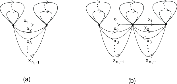
Figure 1: The graph $\Omega$ when (a) $n_{i,j}>0$ is even, (b) $n_{i,j}>1$ is odd.

The method for constructing ${\cal G}_{4}(n)$ breaks into two subcases, i.e.
(a) when $n_{i,j}$ is even,
(b) when $n_{i,j}$ is odd.

Subcase (a): $n_{i,j}$ is even.

Recall that for each $k=1,2$, $p=1,...,b_{k}$, $\cup_{q=1}^{d_{i,k}}\Theta_{k,p,q}(n)$ is a connected path in ${\cal{G}}_{3}(n)^{f}$ representing the word

$$x_{b_{k-1}+p}^{nd_{i}}$$

and thus we can divide the path equally into $d_{i}$ subpaths

$$\Psi_{k,p,a}(n);\;\;\;a=1,...,d_{i}$$

each representing the word

$$x_{b_{k-1}+p}^{n}.$$

Now we pick a vertex $u_{k,p,a}$ in $\Psi_{k,p,a}(n)$ for each $k=1,2,p=1,....,b_{k},a=1,...,d_{i}$ as follows
– if $(k,p)\neq(2,b_{2})$, then $u_{k,p,a}$ is the middle vertex of $\Psi_{k,p,a}(n)$ (recall that $n$ is even);
– if $(k,p)=(2,b_{2})$, then $u_{2,b_{2},a}$ is a vertex around the middle vertex of $\Psi_{k,p,a}(n)$ which is the initial vertex of a $x_{1}$-edge.

By Note 5.15, for each $k=1,2$ and $p=1,...,b_{k}$, the set of $d_{i}$ points

$$\{u_{k,p,a};a=1,...,d_{i}\}$$

is contained in the set of $d_{i,k}$ paths

$$\{\Phi_{k,p,q}(n);q=1,...,d_{i,k}\}.$$

Now we cut ${\cal{G}}_{3}(n)^{f}$ at the vertices $u_{k,p,a}$, $k=1,2,p=1,...,b_{k},a=1,...,d_{i}$, that is, we form a cut graph ${\cal{G}}_{3}(n)^{f}_{c}={\cal{G}}_{3}(n)^{f}\setminus\{u_{k,p,a},k=1,2,p=1,...,b_{k},a=1,...,d_{i}\}$, whose vertex set is obtained from the vertex set of ${\cal{G}}_{3}(n)^{f}$ by replacing each $u_{k,p,a}$ with a pair of vertices $u_{k,p,a}^{\pm}$ (where $u_{k,p,a}^{+}$ is the terminal vertex and $u_{k,p,a}^{-}$ is the initial vertex).

Now we take $d_{i}$ copies of the graph $\Omega$ shown in Figure 1 (a), which we denote by $\Omega_{a}$, $a=1,...,d_{i}$. For each fixed $a=1,...,d_{i}$, we identify the vertex set

$$\{u_{k,p,a}^{\pm},k=1,2,p=1,...,b_{k}\}$$

of ${\cal{G}}_{3}(n)^{f}_{c}$ with the vertices of $\Omega_{a}$ as follows:
– if $(k,p)\neq(2,b_{2})$, identify $u_{k,p,a}^{+}$ with the left vertex of ${\Omega}_{a}$ if $b_{k-1}+p$ is odd and to the right vertex if $b_{k-1}+p$ is even, and identify $u_{k,p,a}^{-}$ with the right vertex of ${\Omega}_{a}$ if $b_{k-1}+p$ is odd and to the left vertex if $b_{k-1}+p$ is even,
– identify $u_{2,b_{2},a}^{+}$ with the left vertex of ${\Omega}_{a}$ and identify $u_{2,b_{2},a}^{-}$ with the right vertex of ${\Omega}_{a}$.

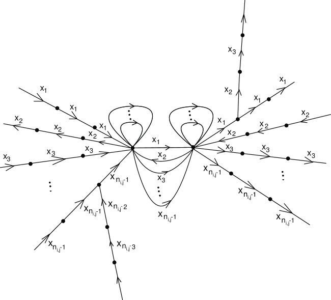
Figure 2:

The resulting graph is not folded, but becomes folded graph after the following obvious folding operation around each inserted ${\Omega}_{a}$:
– fold the subpath $x_{n_{i,j}-1}a_{1}b_{1}a_{1}^{-1}b_{1}^{-1}\cdots a_{g}b_{g}a_{g}^{-1}b_{g}^{-1}$ whose terminal vertex is the vertex $u_{2,b_{2},a}^{+}$ with the loops of ${\Omega}_{a}$ at the left vertex of ${\Omega}_{a}$ and then with the $x_{n_{i,j}-1}$-edge of ${\cal G}_{4}(n)$ whose terminal vertex is the left vertex of ${\Omega}_{a}$, and
– fold the two $x_{1}$-edges whose initial vertices are the right vertex of ${\Omega}_{a}$.
The resulting folded graph, denoted ${\cal G}_{4}(n)$, around the inserted ${\Omega}_{a}$ is shown in Figure 2. By our construction we see that ${\cal G}_{4}(n)$ is a folded, $L$-labeled, directed graph, with no $x_{b}$-loops, with each of the words $w_{1}^{*},...,w_{\ell}^{*}$ still representable by a loop based at $v_{0}$, and with each of the words $y_{1},...,y_{r}$ still representable by a non-closed path based at $v_{0}$. Also we see that the graph ${\cal G}_{4}(n)$ contains loops based $v_{0}$ representing the words

$$z_{k,p,q}(n+1)^{*},\;\;k=1,2,p=1,...,b_{k},q=1,...,d_{i,k}-1.$$

The graph ${\cal G}_{4}(n)$ is not $L$-regular yet since it does not contain any $x_{b}$-loops. So it must contain a missing label. Let $x\in L$ be a missing label at a vertex $v$ of ${\cal G}_{4}(n)$. Let $\alpha$ be a finite directed graph consisting of a single path of edges all labeled with $x$, as shown in Figure 3. We identify the left end vertex of $\alpha$ to the vertex $v$ of ${\cal G}_{4}(n)$. The resulting graph ${\cal G}_{5}(n)$ is obviously still folded, contains ${\cal G}_{4}(n)$ as an embedded subgraph, and contains no $x_{b}$-loops for any $b=1,...,n_{i,j}$. By choosing a long enough path $\alpha$, we may assume that the number of vertices of ${\cal G}_{5}(n)$ is bigger than $(n+1)d_{i}+1$.

Figure 3:

Now by Theorem 5.12, we can obtain an $L$-regular graph ${\cal G}_{6}(n)$ such that
(1) ${\cal G}_{5}(n)$ is an embedded subgraph of ${\cal G}_{6}(n)$; thus in particular in ${\cal G}_{6}(n)$ each of the words $w_{1}^{*},...,w_{\ell}^{*}$, $z_{k.p.q}(n+1)^{*}$, $k=1,2,p=1,...,b_{k}$, $q=1,...,d_{i,k}-1$ is representable by a loop based at $v_{0}$, and each of the words $y_{1},...,y_{r}$ is representable by a non-closed path based at $v_{0}$;
(2) ${\cal G}_{6}(n)$ contains no loops representing the word $x_{b}^{d}$ for any $b=1,...,n_{i,j}$, $d=1,...,m_{*}-1$, where $m_{*}$ is the number of vertices of ${\cal G}_{6}(n)$ (note that $m^{*}$ depends on $i$ and $j$).

Note that $m_{*}$ is some integer larger than $(n+1)d_{i}+1$. Let $N_{i,j}=m_{*}-(d_{i}-1)(n+1)-1$. Then $N_{i,j}>(n+1)$.

During the transformation from ${\cal G}_{4}(n)$ to ${\cal G}_{6}(n)$, the subgraph of ${\cal G}_{4}(n)$ consisting of the edges which intersect the subgraph $\Omega_{a}$ (for each fixed $a=1,...,d_{i}$) remained unchanged since ${\cal G}_{4}(n)$ was locally $L$-regular already at the two vertices of ${\Omega}_{a}$. Now we replace ${\Omega}_{a}$, for each of

$$a=1,...,d_{i}-1,$$

by a graph ${\Omega}_{a}(N_{i,j}-n+1)$ which is similar to $\Omega_{a}$ but with $N_{i,j}-n+1\geq 3$ vertices (Figure 4 illustrates such a graph with four vertices). Then the resulting graph, which we denote by ${\cal G}(N_{i,j})$, has the following properties.
(1) ${\cal G}(N_{i,j})$ is $L$-regular;
(2) each of the words $y_{1},...,y_{r}$ is still representable by a non-closed path based at $v_{0}$ in ${\cal G}(N_{i,j})$,
(3) each of the words $w_{1}^{*},...,w_{\ell}^{*}$ is still representable by a loop based at $v_{0}$ in ${\cal G}(N_{i,j})$,
(4) ${\cal G}(N_{i,j})$ contains no loops representing the word $x_{b}^{d}$ for each $b=1,...,n_{i,j}$ and each $d=1,...,m_{\#}-1$, where $m_{\#}$ is the number of vertices of ${\cal G}(N_{i,j})$,
(5) ${\cal G}(N_{i,j})$ contains a closed loop based at $v_{0}$ representing the word $z_{k,p,q}(N_{i,j})^{*}$, for each $k=1,2,p=1,...,b_{k},q=1,...,d_{i}-1$, and
(6) $m_{\#}$, the number of vertices of ${\cal G}(N_{i,j})$, is equal to $N_{i,j}d_{i}+1$.
Properties (1)-(5) are obvious by the construction, while property (6) follows by a simple calculation. Indeed

$$m_{\#} = m_{*}+(N_{i,j}-n+1-2)(d_{i}-1)$$

$$= [N_{i,j}+(d_{i}-1)(n+1)+1]+(N_{i,j}-(n+1))(d_{i}-1)$$

$$= N_{i,j}d_{i}+1.$$

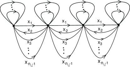
Figure 4:

Now for each integer $N_{*}\geq N_{i,j}$ we construct a finite, connected, $L$-labeled, directed graph ${\cal G}(N_{*})$ (with a fixed base vertex $v_{0}$) with the properties (0)-(5) listed in Theorem 5.10. In the graph ${\cal G}(N_{i,j})$ above, for each $a=1,...,d_{i}-1$, replace the subgraph ${\Omega}_{a}(N_{i,j}-n+1)$ by the graph ${\Omega}_{a}(N_{*}-n+1)$, and replace subgraph ${\Omega}_{d_{i}}$ by the graph ${\Omega}_{d_{i}}(N_{*}-N_{i,j}+2)$. The resulting graph is ${\cal G}(N_{*})$.

Subcase (b) $n_{i,j}>1$ is odd.

We modify the graph ${\cal G}_{3}(n)^{f}$ as follows. Besides the vertices $u_{k,p,a}$ we have chosen before, we choose, for each $a=1,...,d_{i}$, a vertex $u_{2,b_{2},a}^{\prime}$ in the directed subpath $\Psi_{2,b_{2},a}$ such that
– $u_{2,b_{2},a}^{\prime}$ is the initial vertex of an edge with label $x_{2}$,
– $u_{2,b_{2},a}^{\prime}$ appears after the vertex $u_{2,b_{2},a}$ in the directed subpath $\Psi_{2,b_{2},a}$,
– there are precisely five edges with label $x_{1}$ between $u_{2,b_{2},a}$ and $u_{2,b_{2},a}^{\prime}$ in the directed subpath $\Psi_{2,b_{2},a}$ (this is possible as $n$ is large).

Again as $n$ is large, the set of $d_{i}$ vertices $\{u_{2,b_{2},a}^{\prime};a=1,...,d_{i}\}$ is contained in the set of $d_{i,k}$ paths $\{\Phi_{2,b_{2},q}(n);q=1,...,d_{i,k}\}$ (cf. Note 5.15).

Now cut ${\cal{G}}_{3}(n)^{f}$ at the vertices $\{u_{k,p,a},k=1,2,p=1,...,b_{k},a=1,...,d_{i}\}$, and $\{u_{2,b_{2},s}^{\prime},a=1,...,d_{i}\}$, and for each $a=1,...,d_{i}$, insert the graph ${\Omega}_{a}$, which is a copy of the graph $\Omega$ shown in Figure 1 (b). That is, we
(1) Form a cut graph ${\cal{G}}_{3}(n)^{f}_{c}={\cal{G}}_{3}(n)^{f}\setminus\{u_{k,p,a},u_{2,b_{2},a}^{\prime},k=1,2,p=1,...,b_{k},a=1,...,d_{i}\}$, defined as in Subcase (a), with obvious modifications, i.e. we have similarly defined pairs of vertices $u_{k,p,a}^{\pm}$, $u_{2,b_{2},a}^{{}^{\prime}\pm}$ for ${\cal{G}}_{3}(n)^{f}_{c}$ such that if each such $\pm$ pair of vertices are identified, then the resulting graph is the original ${\cal{G}}_{3}(n)^{f}$.
(2) For each fixed $a=1,...,d_{i}$, we identify the vertex set $\{u_{k,p,a}^{\pm},u_{2,b_{2},a}^{{}^{\prime}\pm},k=1,2,p=1,...,b_{k}\}$ of ${\cal{G}}_{3}(n)^{f}_{c}$ with the left-most and right-most vertices of $\Omega_{a}$ as follows:
– if $(k,p)\neq(2,b_{2})$, and $(k,p)=(1,1)$ or $b_{k-1}+p$ is even, then identify $u_{k,p,a}^{+}$ with the left-most vertex of ${\Omega}_{a}$ and $u_{k,p,a}^{-}$ with the right-most vertex.
– if $(k,p)\neq(2,b_{2})$, $(k,p)\neq(1,1)$ and $b_{k-1}+p$ is odd, then identify $u_{k,p,a}^{+}$ with the right-most vertex of ${\Omega}_{a}$ and $u_{k,p,a}^{-}$ with the left-most vertex,
– identify $u_{2,b_{2},a}^{+}$ with the left-most vertex of ${\Omega}_{a}$ and identify $u_{2,b_{2},a}^{-}$ with the right-most vertex of ${\Omega}_{a}$,
– identify $u_{2,b_{2},a}^{{}^{\prime}+}$ with the left-most vertex of ${\Omega}_{a}$ and identify $u_{2,b_{2},a}^{{}^{\prime}-}$ with the right-most vertex of ${\Omega}_{a}$.

The resulting graph is not folded, but becomes folded graph after the following folding operations are performed around each inserted ${\Omega}_{a}$:
– fold the path $x_{n_{i,j}-1}a_{1}b_{1}a_{1}^{-1}b_{1}^{-1}\cdots a_{g}b_{g}a_{g}^{-1}b_{g}^{-1}$ whose terminal vertex is the vertex $u_{2,b_{2},a}^{+}$ with the loops of ${\Omega}_{a}$ at the left-most vertex of ${\Omega}_{a}$ and then with the $x_{n_{i,j}-1}$-edge of ${\cal G}_{4}(n)$ whose terminal vertex is the left-most vertex of ${\Omega}_{a}$,
– fold the two $x_{1}$-edges whose initial vertices are the right-most vertex of ${\Omega}_{a}$,
– fold the two $x_{1}$-edges whose terminal vertices are the left-most vertex of ${\Omega}_{a}$,
– fold the two $x_{2}$-edges whose initial vertices are the right-most vertex of ${\Omega}_{a}$.
The resulting folded graph ${\cal G}_{4}(n)^{f}$ around the inserted ${\Omega}_{a}$ is shown in Figure 5. By our construction we see that ${\cal G}_{4}(n)^{f}$ is a folded, $L$-labeled, directed graph, with no $x_{b}$-loops, with each of the words $w_{1}^{*},...,w_{\ell}^{*}$ still representable by a loop based at $v_{0}$, and with each of the words $y_{1},...,y_{r}$ still representable by a non-closed path based at $v_{0}$. Also we see that the graph ${\cal G}_{4}(n)$ contains loops based $v_{0}$ representing the words $z_{k,p,q}(n+2)^{*}$, for all $k=1,2,p=1,...,b_{k},q=1,...,d_{i,k}-1$.

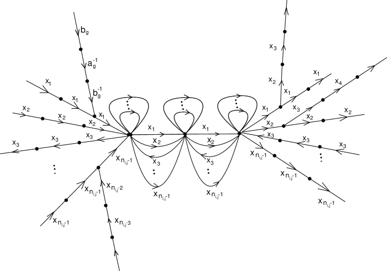
Figure 5:

We then define ${\cal G}_{5}(n)$ and ${\cal G}_{6}(n)$ in a similar manner as in Subcase (a); here we may assume that ${\cal G}_{5}(n)$ has at least $(d_{i}-1)(n+2)-1$ vertices. Let $m_{*}$ be the number of vertices of ${\cal G}_{6}(n)$, and let $N_{i,j}=m_{*}-(d_{i}-1)(n+2)-1$. To form ${\cal G}(N_{i,j})$, we replace each subgraph $\Omega_{a}$, $a=1,...,d_{i}-1$ in ${\cal G}_{6}(n)$ with a graph ${\Omega}_{a}(1+N_{i,j}-n)$ similar to Figure 1(b) but with $1+N_{i,j}-n$ vertices. In the current case, we need $1+N_{i,j}-n$ to be an odd integer in order for the construction to work. This is made possible by the following

Lemma 5.16.

$N_{i,j}-n$ is even, i.e. $N_{i,j}$ is even (since we have chosen $n$ to be even (see Note 5.3)).

The proof of this lemma is similar to that of [MZ, Lemma 11.3], noticing in the current case the number $d_{i}$ is even for each $i=1,2$ by Notation 2.3.

The rest of the argument proceeds by obvious analogy with the Subcase (a). That is, the graph ${\cal G}(N_{i,j})$ is a graph with the properties listed as (1)-(6) in Subcase (a). Indeed, Properties (1)-(5) are immediate. To verify Property (6), we let $m_{\#}$ be the number of vertices of ${\cal G}(N_{i,j})$, and then we have:

$$m_{\#} = m_{*}+(1+N_{i,j}-n-3)(d_{i}-1)$$

$$= N_{i,j}+(d_{i}-1)(n+2)+1+(N_{i,j}-n-2)(d_{i}-1)$$

$$= N_{i,j}d_{i}+1.$$

Now for each even integer $N_{*}\geq N_{i,j}$, the graph ${\cal G}(N_{*})$ required by Theorem 5.10 is obtained from the graph ${\cal G}(N_{i,j})$ by replacing each subgraph ${\Omega}_{a}(N_{i,j}-n+1)$, $a=1,...,d_{i}-1$, by the graph ${\Omega}_{a}(N_{*}-n+1)$, and replacing the subgraph ${\Omega}_{d_{i}}$ by the graph ${\Omega}_{d_{i}}(N_{*}-N_{i,j}+3)$.

Proof of Theorem 5.1 in Case 2.

The proof is similar to that of Case 1 and much simpler notationally, and we shall be very brief. In this case $n_{i,j}=1$, i.e. the surface $S_{i,j}$ has only one boundary component, which we denote by $\beta$ and may assume lying in $T_{1}$. $\beta$ has $d_{i,1}$ intersection points with ${\partial}S_{i_{*}}$, which we denote by $t_{q}$, $q=1,...,d_{i,1}$. Similarly as in Case 1, we define the points $b_{q},q=1,...,d_{i,1}$ in ${\partial}_{p}J_{i,j}$. The group $\pi_{1}(S_{i,j}^{-},t_{1})$ has a set of generators

$$L=\{a_{1},b_{1},...,a_{g},b_{g}\}$$

($g$ must be larger than $0$) such that

$$x_{1}=a_{1}b_{1}a_{1}^{-1}b_{1}^{-1}\cdots a_{g}b_{g}a_{g}^{-1}b_{g}^{-1}$$

is an embedded loop which is homotopic to $\beta$. As in Case 1, we similarly define the elements $w_{1},...,w_{\ell}$, the element $y_{1},...,y_{r}$, and the elements $z_{q}(n)$, $q=1,...,d_{i,1}-1$, and we reduce the proof of Theorem 5.1 in Case 2 to the proof of the following theorem which is an analogue of Theorem 5.10.

Theorem 5.17.

There is a positive even integer $N_{i,j}$ such that for each even integer $N_{*}\geq N_{i,j}$ there is a finite, connected, $L$-labeled, directed graph ${\cal G}(N_{*})$ (with a fixed base vertex $v_{0}$) with the following properties:
(0) ${\cal G}(N_{*})$ is $L$-regular;
(1) The number of vertices of ${\cal G}(N_{*})$ is $m_{i}=N_{*}d_{i}+1$;
(2) Each of the words $w_{1}^{*},...,w_{\ell}^{*}$ is representable by a loop, based at $v_{0}$, in ${\cal G}(N_{*})$;
(3) ${\cal G}(N_{*})$ contains a closed loop, based at $v_{0}$, representing the word $z_{q}(N_{*})^{*}$, for each $q=1,...,d_{i,1}-1$;
(4) ${\cal G}(N_{*})$ contains no loop representing the word $x_{1}^{d}$ for any $d=1,...,m_{i}-1$;
(5) each of the words $y_{1},...,y_{r}$ is representable by a non-closed path, based at $v_{0}$, in ${\cal G}(N_{*})$.

To prove this theorem, we construct, similar as in Case 1, the analogue graph ${\cal G}_{3}(n)^{f}$ and its subgraphs $\Phi_{q}(n),q=1,...,d_{i,1}$, $\Psi_{a}(n),a=1,...,d_{i}$, with similar properties. We modify the graph ${\cal G}_{3}(n)^{f}$ as follows. For each of $a=1,...,d_{i}$, we pick a pair vertices $\{u_{a},u_{a}^{\prime}\}$ in the path $\Psi_{a}(n)$ as follows:
–$u_{a}$ is closed to the middle vertex of $\Psi_{a}(n)$;
–$u_{a}$ is the terminal vertex of an edge with label $a_{1}$; and
–$u_{a}^{\prime}$ is the terminal vertex of an edge with label $b_{1}$ which appears after the vertex $u_{a}$;
–there are precisely five edges with label $b_{1}$ between $u_{a}$ and $u_{a}^{\prime}$ in the path $\Psi_{a}(n)$.

We may assume that the set

$$\{u_{a},u_{a}^{\prime};a=1,...,d_{i}\}$$

is contained in the set

$$\{\Phi_{q}(n);q=1,...,d_{i,1}\}.$$

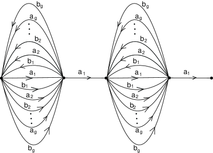
Figure 6:

Now cut the graph ${\cal{G}}_{3}(n)^{f}$ at all the pairs of vertices $\{u_{a},u_{a}^{\prime}\}$, $a=1,...,d_{i}$, and for each $a$, insert the graph ${\Omega}_{a}$– which is a copy of the graph $\Omega$ shown in Figure 6 – as follows. Form a cut graph ${\cal{G}}_{3}(n)^{f}_{c}={\cal{G}}_{a}(n)^{f}\setminus\{u_{a},u_{a}^{\prime};a=1,...,d_{i}\}$, and let $u_{a}^{\pm}$, $u_{a}^{{}^{\prime}\pm}$ be the corresponding vertices for ${\cal{G}}_{3}(n)^{f}_{c}$. For each fixed $a=1,...,d_{i}$, we identify the vertex $u_{a}^{+}$ with the left-most vertex of ${\Omega}_{a}$, identify $u_{a}^{-}$ with the right-most vertex of ${\Omega}_{a}$, identify $u_{a}^{{}^{\prime}+}$ with the right-most vertex of ${\Omega}_{a}$ and identify $u_{a}^{{}^{\prime}-}$ with the left-most vertex of ${\Omega}_{a}$.

The resulting graph is not folded, but becomes folded graph after a single folding operation around each inserted ${\Omega}_{a}$: fold the two $a_{1}$-edges whose terminal vertices are the right-most vertex of ${\Omega}_{a}$. The resulting folded graph ${\cal G}_{4}(n)^{f}$ around the inserted ${\Omega}_{a}$ is shown in Figure 7. By our construction we see that ${\cal G}_{4}(n)^{f}$ is a folded $L$-labeled directed graph, with no $x_{1}$-loops, with each of the words $w_{1}^{*},...,w_{\ell}^{*}$ still representable by a loop based at $v_{0}$, and with each of the words $y_{1},...,y_{r}$ still representable by a non-closed path based at $v_{0}$. Also we see that the graph ${\cal G}_{4}(n)$ contains loops based at $v_{0}$ representing the words $z_{q}(n+4)^{*}$, for all $q=1,...,d_{i,1}-1$.

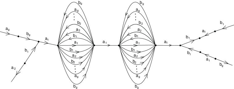
Figure 7:

As in Case 1, we get ${\cal G}_{5}(n)$ and ${\cal G}_{6}(n)$. In the current case, $N_{i,j}=m_{*}-(d_{i}-1)(n+4)-1$, which is larger than $n+4$, where $m_{*}$ is the number of vertices of ${\cal G}_{6}(n)$. To form ${\cal G}(N_{i,j})$, we replace the left half (with three vertices) of $\Omega_{a}$, for each $a=1,...,d_{i}-1$, with a graph ${\Omega}_{a}(N_{i,j}-n-1)$ which is similar to Figure 6 but with $N_{i,j}-n-1$ vertices. In the current case, we also need $N_{i,j}$ to be an even integer in order for the construction to work. This is true, and can be proved as in Subcase (b) of Case 1. It is easy to see that ${\cal G}(N_{i,j})$ has all the Properties (0)-(5) listed in Theorem 5.17 (when $N_{*}=N_{i,j}$). For instance to check Property (1), we have:

$$m_{i} = m_{*}+(N_{i,j}-n-1-3)(d_{i}-1)$$

$$= N_{i,j}+(d_{i}-1)(n+4)+1+(N_{i,j}-n-4)(d_{i}-1)$$

$$= N_{i,j}d_{i}+1$$

To show that Theorem 5.17 holds for any even integer $N_{*}\geq N_{i,j}$, we simply let ${\cal G}(N_{*})$ be the graph obtained from the graph ${\cal G}(N_{i,j})$ by replacing each subgraph ${\Omega}_{a}(N_{i,j}-n-1)$, $a=1,...,d_{i}-1$, by the graph ${\Omega}_{a}(N_{*}-n-1)$, and replacing the subgraph ${\Omega}_{d_{i}}$ by the graph ${\Omega}_{d_{i}}(N_{*}-N_{i,j}+5)$.

6 The final assembly

Fix an even integer $N_{*}$ satisfying Corollary 5.2 (later on we may need $N_{*}$ to have been chosen large enough). Then as given in Corollary 5.2, for each $i=1,2$ and $j=1,..,n_{i}$, the manifold $Y_{i,j}^{-}=S_{i,j}^{-}\times I$ has an $m_{i}=N_{*}d_{i}+1$ fold cover $\breve{Y}_{i,j}^{-}=\breve{S}_{i,j}^{-}\times I$ such that $|{\partial}_{p}\breve{Y}_{i,j}^{-}|=|{\partial}_{p}Y_{i,j}^{-}|$, i.e. each component of ${\partial}_{p}\breve{Y}_{i,j}^{-}$ is an $m_{i}$ fold cyclic cover of a component of ${\partial}_{p}Y_{i,j}^{-}$. Moreover the map $g_{i,j}:(J_{i,j}^{-},{\partial}_{p}J_{i,j}^{-}){\rightarrow}(Y_{i,j}^{-},{\partial}_{p}Y_{i,j}^{-})$ lifts to an embedding $\breve{g}_{i,j}:(J_{i,j}^{-},{\partial}_{p}J_{i,j}^{-}){\rightarrow}(\breve{Y}_{i,j}^{-},{\partial}_{p}\breve{Y}_{i,j}^{-})$ such that if $\breve{A}$ is a component of ${\partial}_{p}\breve{Y}_{i,j}^{-}$ then the components of $\breve{g}_{i,j}({\partial}_{p}J_{i,j}^{-})\cap\breve{A}$ are evenly distributed along $\breve{A}$. More precisely if $S_{i,j}^{-}$, for instance, is the surface given in the proof of Theorem 5.1 in Case 1, then with the notations given there, we may index the boundary components of $\breve{S}_{i,j}^{-}$ as $\breve{\beta}_{k,p}$, $k=1,2,p=1,...,b_{k}$, so that each $\breve{\beta}_{k,p}$ is an $m_{i}$ fold cyclic cover of $\beta_{k,p}$ and the points $\{\breve{g}_{i,j}(b_{k,p,q});q=1,....,d_{i,k}\}$ divide $\breve{\beta}_{k,p}$ into $d_{i,k}$ segments each having wrapping number $N_{*}d_{i}/d_{i,k}$. Also note that the $d_{i,k}$ points $\{\breve{g}_{i,j}(b_{k,p,q});q=1,....,d_{i,k}\}$ are mapped to the $d_{i,k}$ points $\{t_{k,p,q};q=1,....,d_{i,k}\}$ respectively under the covering map $\breve{\beta}_{k,p}{\rightarrow}\beta_{k,p}$. As $N_{*}$ can be assumed to be arbitrarily large, we may assume that the wrapping number $N_{*}d_{i}/d_{i,k}$ be as large as needed for each $i=1,2$ and $k=1,...,m$.

Also recall that $(K_{i,j}^{-},{\partial}_{p}K_{i,j}^{-})$ is properly embedded in the pair $(J_{i,j}^{-},{\partial}_{p}J_{i,j}^{-})$, with a relative $R$-collared neighborhood. It follows that the pair $(\breve{g}_{i,j}(K_{i,j}^{-}),\breve{g}_{i,j}({\partial}_{p}K_{i,j}^{-}))$ has a relative $R$-collared neighborhood in $(\breve{Y}_{i,j}^{-},{\partial}_{p}\breve{Y}_{i,j}^{-})$. Also $K_{1}^{-}=\cup_{j=1}^{n_{1}}K_{1,j}$ and $K_{2}^{-}=\cup_{j=1}^{n_{2}}K_{2,j}$ are isometric under the isometry $h:K_{1}{\rightarrow}K_{2}$. Now let $\breve{Y}^{-}$ be the union of $\breve{Y}_{1}^{-}=\cup_{j=1}^{n_{1}}Y_{1,j}^{-}$ and $\breve{Y}_{2}^{-}=\cup_{j=1}^{n_{2}}Y_{2,j}^{-}$ with $\cup_{j=1}^{n_{1}}(\breve{g}_{1,j}(K_{1,j}^{-}),\breve{g}_{1,j}({\partial}_{p}K_{1,j}^{-}))$ and $\cup_{j=1}^{n_{2}}(\breve{g}_{2,j}(K_{2,j}^{-}),\breve{g}_{2,j}({\partial}_{p}K_{2,j}^{-}))$ identified by the corresponding isometry and let $(U^{-},{\partial}_{p}U^{-})$ be the identification space of $\cup_{j=1}^{n_{1}}(\breve{g}_{1,j}(K_{1,j}^{-}),\breve{g}_{1,j}({\partial}_{p}K_{1,j}^{-}))$ and $\cup_{j=1}^{n_{2}}(\breve{g}_{2,j}(K_{2,j}^{-}),\breve{g}_{2,j}({\partial}_{p}K_{2,j}^{-}))$ in $\breve{Y}^{-}$. Then $\breve{Y}^{-}$ is a connected metric space, with a path metric induced from the metrics on $\breve{Y}_{1}^{-}$ and $\breve{Y}_{2}^{-}$. There is an induced local isometry $f:\breve{Y}^{-}{\rightarrow}M$ which extends the local isometry $\breve{Y}_{i,j}^{-}{\rightarrow}Y_{i,j}^{-}{\rightarrow}M$ for each $i,j$.

Define the parabolic boundary, ${\partial}_{p}\breve{Y}^{-}$, of $\breve{Y}^{-}$ to be the union of ${\partial}_{p}\breve{Y}_{1}^{-}$ and ${\partial}_{p}\breve{Y}_{2}^{-}$, with $\cup_{j=1}^{n_{1}}\breve{g}_{1,j}({\partial}_{p}K_{1,j}^{-})$ and $\cup_{j=1}^{n_{2}}\breve{g}_{2,j}({\partial}_{p}K_{2,j}^{-})$ identified by the isometry. Then $(U^{-},{\partial}_{p}U^{-})$ has a relative $R$-collared neighborhood in $(\breve{Y}^{-},{\partial}_{p}\breve{Y}^{-})$.

Now for each $k=1,...,m$, let $\breve{C}_{K}$ be the cover of the $k$-th cusp $C_{k}$ of $M$ corresponding to the subgroup of $\pi_{1}(C_{k})$ generated by the $m_{1}$-th power of a component of ${\partial}_{k}S_{1}^{-}$ and the $m_{2}$-th power of a component of ${\partial}_{k}S_{2}^{-}$. Then each oriented component, say $\beta$, of ${\partial}_{k}S_{i}^{-}$ has its inverse image in ${\partial}\breve{C}_{k}$, denoted $\breve{\beta}$, a connected oriented circle. So we may and shall identify $\breve{\beta}$ with the oriented component of ${\partial}\breve{S}_{i}^{-}$ which covers $\beta$. This way we embed naturally all components of ${\partial}\breve{S}_{i}^{-}$ into ${\partial}\breve{C}=\cup_{k=1}^{m}{\partial}\breve{C}_{k}$, for each $i=1,2$. We denote by ${\partial}_{k}\breve{S}_{i}^{-}$ those components of ${\partial}\breve{S}_{i}^{-}$ which are embedded in ${\partial}\breve{C}_{k}$. Then we have $|{\partial}_{k}\breve{S}_{i}^{-}|=|{\partial}_{k}S_{i}|$, and the components of ${\partial}_{k}\breve{S}_{i}^{-}$ are far apart from each other in ${\partial}\breve{C}_{k}$, for each $i=1,2$ and $k=1,...,m$. So we may and shall embed the corresponding components of ${\partial}_{p}\breve{Y}_{i}^{-}$ into ${\partial}\breve{C}$ along ${\partial}\breve{S}_{i}^{-}$, for each $i=1,2$. After such identification, we get a connected hyperbolic $3$-manifold

$$\breve{Y}^{-}\cup(\cup_{k=1}^{m}\breve{C}_{k})$$

with $m$ rank two cusps and with a local isometry into $M$.

As in [MZ, Section 13] we construct the thickening $\bar{U}^{-}$ of $U^{-}$ so that ${\partial}_{p}\bar{U}$ is embedded in ${\partial}\breve{C}$ (Note that each component of $\bar{U}^{-}$ is a handlebody, with a similar proof as that of [MZ, Lemma 13.2]) and let

$$Y^{-}=\breve{Y}_{1}^{-}\cup\bar{U}^{-}\cup\breve{Y}_{2}^{-}.$$

Then $Y^{-}$ is a connected, compact, hyperbolic $3$-manifold, locally convex everywhere except on its parabolic boundary ${\partial}_{p}Y^{-}={\partial}_{p}\breve{Y}_{1}^{-}\cup{\partial}_{p}\bar{U}^{-}\cup{\partial}_{p}\breve{Y}_{2}^{-}$. The complement of ${\partial}_{p}(Y^{-})$ in ${\partial}\breve{C}$ is a set of “round-cornered parallelograms” with very long sides in ${\partial}\breve{C}$. As in [MZ, Section 13], we scoop out from $\breve{C}=\cup_{k=1}^{m}C_{k}$ the convex half balls based on these round-cornered Euclidean parallelograms and denote the resulting cusps by $\cup_{k=1}^{m}\breve{C}_{k}^{0}$. Then

$$Y=Y^{-}\cup(\cup_{k=1}^{m}\breve{C}_{k}^{0})$$

is a connected, metrically complete, convex hyperbolic $3$-manifold, with a local isometry $f$ into $M$. Thus the local isometry $f$ induces an injection of $\pi_{1}(Y)$ into $\pi_{1}(M)$ by [MZ, Lemma 4.2].

Each boundary component of $Y$ provides a Quasi-Fuchsian surface in $M$. To prove this claim, it suffices to show, with a similar reason as that given in [MZ, Section 13], that every Dehn filling of $Y$ along its cusps gives a $3$-manifold with incompressible boundary.

Let $Y(\alpha_{1},...,\alpha_{m})$ be any Dehn filling of $Y$ with slopes $\alpha_{1},...,\alpha_{m}$. Then $Y(\alpha_{1},...,\alpha_{m})$ is an $HS$-manifold (see [MZ, Section 12] for its definition). The handlebody part $H$ of $Y(\alpha_{1},...,\alpha_{m})$ is $\bar{U}^{-}\cup(\cup_{k=1}^{m}\breve{C}_{k}^{0}(\alpha_{k}))$ (which may have several components in the current case but each has genus at least two) and the $S\times I$ part of $Y(\alpha_{1},...,\alpha_{m})$ is $Y(\alpha_{1},...,\alpha_{m})\setminus H=Y^{-}\setminus\bar{U}^{-}$. This $HS$ decomposition of $Y(\alpha_{1},...,\alpha_{m})$ satisfies the conditions of [MZ, Lemma 12.1] and thus $Y(\alpha_{1},...,\alpha_{m})$ has incompressible boundary by that lemma. The proof of this last claim is similar to that of [MZ, Lemma 13.6], for which we only need to note the following:
(1) With a similar proof as that of [MZ, Lemma 13.5] we have that each component of $Y^{-}\setminus\bar{U}^{-}$ is not simply connected.
(2) $|{\partial}_{k}\breve{S}^{-}_{i}|=|{\partial}_{k}S_{i}^{-}|\geq 2$ for each $i=1,2,k=1,...,m$, by Condition 2.2.

The proof of Theorem 1.1 is now finished.

References

- [CL] D. Cooper and D. D. Long, Some surface subgroups survive surgery, Geom. Topol. 5 (2001) 347–367 (electronic).
- [CS] M. Culler and P. B. Shalen, Bounded, separating, incompressible surfaces in knot manifolds, Invent. Math. 75 (1984) 537–545.
- [MZ] J. Masters and X. zhang, Closed quasi-Fuchsian surfaces in hyperbolic knot complements, Geometry & Topology 12 (2008) 2095-2171
- [T] W. Thurston, The Geometry and Topology of Three Manifolds, lecture notes, Princeton, 1979.