Critical percolation: the expected number of clusters in a rectangle

Abstract

We show that for critical site percolation on the triangular lattice two new observables have conformally invariant scaling limits. In particular the expected number of clusters separating two pairs of points converges to an explicit conformal invariant. Our proof is independent of earlier results and $SLE$ techniques, and in principle should provide a new approach to establishing conformal invariance of percolation.

1 Introduction

Percolation is perhaps the easiest two-dimensional lattice model to formulate, yet it exhibits a very complicated behavior. A number of spectacular predictions (unrigorous, but very convincing) appeared in the physics literature over the last few decades, see [3]. One of them, the Cardy’s formula for the scaling limit of crossing probabilities, was recently established for the critical site percolation on triangular lattice [10]. Consequently, scaling limits of interfaces were identified with Schramm’s $SLE_{6}$ curves, and many other predictions were proved, see e.g. [14].

In this paper we show that two new observables for the critical site percolation on triangular lattice have conformally invariant scaling limits. Furthermore, we obtain explicit formulae, consistent with predictions obtained by physicists [4, 9]. Our proof is independent of earlier conformal invariance results, and uses methods similar to those in [10] rather than $SLE$ techniques. It is also restricted to the same triangular lattice model, but at least one should be able to use it for a new proof of the conformal invariance in this case.

1.1 Acknowledgements

The first author would like to thank Thomas Mountford and Yvan Velenik for useful discussions and remarks. This work was supported by the Swiss National Science Foundation grants 117596, 117641, 121675. The first author was partially supported by an EPFL Excellence Scholarship.

2 Notation and Setup

For convenience reasons, in this paper we shall not work on the triangular lattice but rather on its dual, the honeycomb lattice, and thus, rather than coloring vertices of triangles, we shall color hexagonal faces (which is obviously equivalent).

2.1 Graph and Model

Let $\Omega\subset\mathbb{C}$ be a Jordan domain (whose boundary is a simple closed curve), and orient its boundary $\partial\Omega$ counterclockwise. Let $l$ and $r$ be two distinct points on $\partial\Omega$, which separate it into a curve $u$ going from $r$ to $l$ (with respect to the orientation of $\partial\Omega$) and a curve $d$ going from $l$ to $r$, such that we have $\partial\Omega\setminus\{l,r\}=u\cup d$. Let finally $w$ be a point on $u$.

Remark 1.

The assumption on $\Omega$ to be a Jordan domain is not really necessary, and the result remains true under weaker assumptions detailed in Section 3. We use this assumption in Section 5 to avoid lengthy and not so interessant discussions.

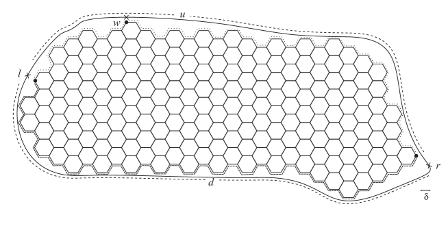
Figure 1: Domain discretization: the points are marked with crosses, while their discretization are marked with circles. The discretization of $u$ and $d$ are depicted by sparse and dense dashes respectively.

We consider the discretization $\Omega_{\delta}$ of $\Omega$ by regular hexagons defined as follows. Let $G_{\delta}$ be the regular hexagonal lattice embedded in the complex plane with mesh size (i.e. sidelength of a hexagon) $\delta>0$. We define $\Omega_{\delta}$ as the graph obtained by taking a maximal connected component made of hexagonal faces of $G_{\delta}$: the union of the closure of the faces is a simply connected subset of $\mathbb{C}$. We denote by $\bar{\Omega}_{\delta}$ this subset and by $\partial\Omega_{\delta}$ the (counterclockwise-oriented) simple path consisting in edges of $\Omega_{\delta}$ such that $\Omega_{\delta}$ is contained inside it. We define the discretization of $l$, $r$ and $w$ as the closest corresponding vertices of $\partial\Omega_{\delta}$, and $u$ and $d$ as the paths from $r$ to $l$ and $l$ to $r$ respectively, following the orientation of $\partial\Omega_{\delta}$. In general we will identify $l,r,u,d$ to their respective discretizations.

We are interested in the process of critical percolation on the faces of $\Omega_{\delta}$: each face of $\Omega_{\delta}$ is colored either in white or in black with probability $\frac{1}{2}$, independently of the other faces; such a coloring is called a configuration. More precisely, we are interested in the scaling limit of this model: the description of the global geometry of the process as the mesh size $\delta$ tends to $0$.

Note that for this model $\frac{1}{2}$ is known to be the critical value for the probability thanks to the work of Wierman and Kesten. However, we do not use that this value is critical, only that it is self-dual.

We call path of hexagons a sequence $\mathcal{H}_{1},\ldots,\mathcal{H}_{n}$ of hexagons such that $\mathcal{H}_{i}$ is adjacent to $\mathcal{H}_{i+1}$ for $i=1,\ldots,n-1$; a path is called simple if all of its hexagons are distinct; a closed simple path (the last hexagon is adjacent to the first one) is called a circuit. We say that a hexagon $\mathcal{H}$ is connected to $u$ by a white path if there exists a path of white hexagons that contains $\mathcal{H}$ and that hits $u$ (contains a hexagon having an edge belonging to (the discretization of) $u$). We define similarly connection events involving black instead of white paths or connections to $d$ instead of $u$. We say that a path of hexagons $\gamma$ separates two families of points $A$ and $B$ if the interior of each continuous path $\alpha$ contained in $\bar{\Omega}_{\delta}$ from a point of $A$ to a point of $B$ crosses the closure of a hexagon of $\gamma$.

We call white cluster a connected (i.e. path-connected in the sense defined above) set of white hexagons. For a cluster $K$ touching $u$ and $d$, we define its left boundary (respectively right boundary) as the left-most (respectively right-most) simple path contained in $K$ that touches $u$ and $d$, i.e. such that there is no path in $K$ separating it from $l$ (respectively $r$); elementary topological considerations show that this notion is well-defined. One important property of our lattice is indeed its self-duality: the boundary of a white cluster (that does not touch the boundary) is a black circuit, and vice versa.

We will use the term left boundary for simplicity, but strictly speaking our definition gives the left-most simple curve inside the cluster, that is its left-most boundary after “peninsulas” attached by only one hexagon are erased. So this curve would rather bound on the right the dual cluster bordering ours on the left.

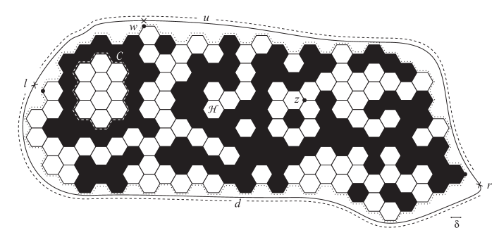
Figure 2: In this configuration, the dashed region $C$ is a white cluster, the hexagon $\mathcal{H}$ is connected to $u$ by a white path and the points $l$ and $w$ are separated from the points $z$ and $r$ by a black path.

Notice that since the probability for a hexagon to be white is $\frac{1}{2}$, any event (i.e. set of configurations) has the same probability as its negative with respect to the colors: for instance, the probability that there is a white path from $x$ to $y$ is the same as the one that there is a black path from $x$ to $y$. For an event $A$, we will denote by $\tilde{A}$ the negative event: a configuration $\omega$ belongs to $A$ if and only if the negative configuration $\tilde{\omega}$ (i.e. with the colors black and white flipped) belongs to $\tilde{A}$.

2.2 Observables

Let $\delta>0$ and consider the process of percolation on $\Omega_{\delta}$ as described in the previous section. For each $z$ vertex of $\Omega_{\delta}$ we define the following random variables and events:

• $N_{\delta}^{l}(z)$: the number of (simple) left boundaries of white clusters touching $u$ and $d$ separating $l$ and $w$ from $z$ and $r$ minus the number of (simple) left boundaries of white clusters (touching $u$ and $d$) separating $l$ and $z$ from $w$ and $r$;

• $N_{\delta}^{r}(z)$: the same as $N_{\delta}^{l}(z)$ but for (simple) right boundaries of white clusters (also touching $u$ and $d$);

• $Q_{\delta}^{u}(z)$: the event that there exists a white simple path from $d$ to $d$ that separates $z$ from $l$ and $r$ and that is connected to $u$;

• $Q_{\delta}^{d}(z)$: the same event as $Q_{\delta}^{u}(z)$ but with a white simple path path from $u$ to $u$ connected to $d$ instead.

This allows us to define our observables:

$$H_{\delta}^{l}(z):=\mathbb{E}[N_{\delta}^{l}(z)], H_{\delta}^{r}(z):=\mathbb{E}[N_{\delta}^{r}(z)],$$

$$H_{\delta}^{u}(z):=\mathbb{P}[Q_{\delta}^{u}(z)], H_{\delta}^{d}(z):=\mathbb{P}[Q_{\delta}^{d}(z)].$$

We extend these functions to continuous functions on $\bar{\Omega}_{\delta}$ in the following way (in fact any reasonable manner will work): first for the center of a hexagon, take the average value of its vertices. Then divide the hexagon into six equilateral triangles, and define the functions on each triangle by affine interpolation. We can then extend the functions to $\bar{\Omega}$ in a smooth way.

Remark 2.

The point $w$ could in fact be anywhere in $\bar{\Omega}$ (changing its position only modifies the functions $H_{\delta}^{l}$ and $H_{\delta}^{r}$ by an additive constant). In our setup it lies on the boundary for simplicity.

Remark 3.

Another way of writing $H_{\delta}^{l}$ (similarly for $H_{\delta}^{r}$), which motivates its definition, is the following: count the expected number of left boundaries that separate $l$ from $z$ and $r$ minus the expected number of left boundaries that separate $l$ from $w$ and $r$.

It is easy to check that this definition is equivalent to the one given above (the boundaries that count positively are precisely the ones that separate $l$ from $r$ and $z$ but not $w$, the boundaries that count negatively are the ones that separate $l$ from $r$ and $w$ but not $z$).

If one uses this way to write $H_{\delta}^{l}$, taking the difference is essential to get a finite limit: as the mesh tends to $0$ the expected number of clusters joining $u$ to $d$ blows up.

Remark 4.

Notice that the quantities $H_{\delta}^{l}$ and $H_{\delta}^{r}$ are the same: if one has a configuration in $\{N_{\delta}^{l}(z)=k\}$, flipping the colors of all the hexagons gives a configuration in $\{N_{\delta}^{r}(z)=k\}$.

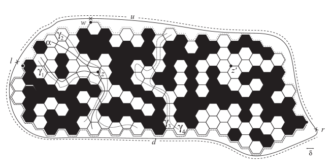
Figure 3: In this configuration, $\gamma_{1}$ and $\gamma_{3}$ are left boundaries of white clusters, $\gamma_{2}$ and $\gamma_{4}$ are right boundaries. $Q_{\delta}^{d}(z)$ occurs and we have $N_{\delta}^{l}(z)=0,N_{\delta}^{r}(z)=-1$ and $N_{\delta}^{l}(z^{\prime})=N_{\delta}^{r}(z^{\prime})=1$.

3 Conformal invariance and main result

By conformal invariance of critical percolation we mean that the same observable on two conformally equivalent Riemann surfaces has the same scaling limit.

It was proven in [10] that crossing probabilities of conformal rectangles (here the Riemann surface is a simply connected domain with four marked boundary points) are conformally invariant and satisfy Cardy’s prediction.

Consequently the interfaces of macroscopic clusters converge to Schramm’s SLE curves and we can deduce conformal invariance of many other observables.

The goal of this paper is to show conformal invariance of the observables $H_{\delta}^{l}+H_{\delta}^{r}$ and $H_{\delta}^{u}-H_{\delta}^{d}$ in the same setup, without appealing to the results of [10].

3.1 Limit of the observables

In order to get our conformal invariance result, we prove a more geometrical one: a linear combination of our two observables turns out to be (in the limit) a conformal mapping. For each $\delta>0$, define $H_{\delta}:=(H_{\delta}^{l}+H_{\delta}^{r})-\frac{\sqrt{3}}{2}i(H_{\delta}^{u}-H_{\delta}^{d})$. Then we have:

Theorem 1.

As $\delta$ tends to $0$, $H_{\delta}$ converges uniformly on the compact subsets of $\bar{\Omega}\setminus\{l,r\}$ to a function $h$ which is the unique conformal mapping from $\Omega$ to the strip $S:=\{x+iy:x\in\mathbb{R},y\in(-\sqrt{3}/4,\sqrt{3}/4)\}$ that maps (in the sense of prime ends) $l$ to the left end of the strip , $r$ to the right end of the strip and $w$ to $\frac{\sqrt{3}}{4}i$.

Remark 5.

The theorem remains valid under the weaker assumption that the discretizations $\Omega_{\delta}$ of the domain converge in Caratheodory’s sense to $\Omega$, in which case the observables converge on the compact subsets of $\Omega$.

This theorem gives us the asymptotical conformal invariance (and the existence of the limit) of the two observables $H_{\delta}^{l}+H_{\delta}^{r}$ and $H_{\delta}^{u}-H_{\delta}^{d}$ in the following sense.

Corollary 1.

Let $\Phi$ be a conformal map as above and denote by $\tilde{H}_{\delta}^{l}$, $\tilde{H}_{\delta}^{r}$, $\tilde{H}_{\delta}^{u}$ and $\tilde{H}_{\delta}^{d}$ the corresponding observables on the domain $\Omega^{\prime}:=\Phi(\Omega)$ with the corresponding points $l^{\prime}:=\Phi(l),r^{\prime}:=\Phi(r),w^{\prime}:=\Phi(w)$. Then we have the following conformal invariance result:

$$\lim_{\delta\to 0}H_{\delta}^{l}+H_{\delta}^{r} = \lim_{\delta\to 0}(\tilde{H}_{\delta}^{l}+\tilde{H}_{\delta}^{r})\circ\Phi$$

$$\lim_{\delta\to 0}H_{\delta}^{u}-H_{\delta}^{d} = \lim_{\delta\to 0}(\tilde{H}_{\delta}^{u}-\tilde{H}_{\delta}^{d})\circ\Phi$$

Proof.

By uniqueness of the conformal mapping to $S$ with three points fixed we have $h=h^{\prime}\circ\Phi$ (the images of $l$, $r$ and $w$ by $h$ and $h^{\prime}\circ\Phi$ are the same). Taking the real and imaginary parts gives the result. ∎

Taking $z$ and $w$ on the boundary we obtain the conformal invariance of the expected number of clusters in a conformal rectangle (a Jordan domain with four distinct points on its boundary). Let $\Xi$ be a conformal rectangle with the four points $a_{1},a_{2},a_{3},a_{4}$ in counterclockwise order. Discretize the domain and the four points as before and consider the expected number $C_{\delta}$ of white clusters separating $a_{1}$ and $a_{4}$ from $a_{2}$ and $a_{3}$, counted in the following way:

• If a cluster touches both (the discretization of) the arcs $a_{4}a_{1}$ and $a_{2}a_{3}$ (along the counterclockwise orientation of the $\partial\Xi$), it does not count.

• If a cluster touches exactly one of the arcs $a_{4}a_{1}$ and $a_{2}a_{3}$, it counts once.

• If it does not touch any of the two arcs, it counts twice.

Corollary 2.

The quantity $C_{\delta}$ admits a conformally invariant limit as $\delta\to 0$: If $\Xi^{\prime}$ is another conformal rectangle with the four points $a_{1}^{\prime},a_{2}^{\prime},a_{3}^{\prime},a_{4}^{\prime}$, if $\Psi:\Xi\to\Xi^{\prime}$ is a conformal mapping such that $\Psi(a_{i})=a_{i}^{\prime}$ for $i=1,2,3,4$, and $C_{\delta}^{\prime}$ is the corresponding number in the domain $\Xi^{\prime}$, then

$$\lim_{\delta\to 0}C_{\delta}=\lim_{\delta\to 0}C_{\delta}^{\prime}$$

Proof.

It suffices to take $z$ on the boundary (choose $z=a_{1},w=a_{2},l=a_{3},r=a_{4}$) and to see that in this case $C_{\delta}=H_{\delta}^{l}+H_{\delta}^{r}$: no clusters count negatively, if a cluster does not touch any arc, both its left and right boundaries count, etc. Therefore the result follows from the previous corollary. ∎

3.2 Formulae

It is not difficult to express the quantity $C_{\delta}$ in terms of the cross-ratio (the conformal map from the half-plane to a strip is simply a logarithm). If we denote by $\lambda=\frac{(a_{1}-a_{3})(a_{2}-a_{4})}{(a_{1}-a_{4})(a_{2}-a_{3})}$ the cross-ratio of the four points, we get

$$\lim_{\delta\to 0}C_{\delta}=\frac{\sqrt{3}\pi}{2}\log\left(\frac{1}{1-\lambda}\right).$$

By adding to this formula the probability that a cluster (separating $a_{4}$ and $a_{1}$ from $a_{2}$ and $a_{3}$) touches the arc $a_{4}a_{1}$ and the probability that such a cluster touches moreover the arc $a_{2}a_{3}$ one can obtain (twice) the expected number of clusters without specific counting.

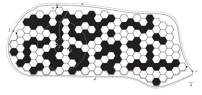
Figure 5: The event $Q_{\delta}^{u}(z)\setminus Q_{\delta}^{u}(z^{\prime})$ implies a black connection of a microscopic circle of radius $\ell(|z-z^{\prime}|)$ to a macroscopic circle of radius $\beta$ ($K$ is not fixed precisely on this picture).

Using self-duality one can show that these two quantities are the same and that they can be expressed as the difference of the probability that a cluster separates $a_{4}$ and $a_{1}$ from $a_{2}$ and $a_{3}$ minus one half times the probability that a cluster touches the four sides of our conformal rectangle: if there is a black cluster separating $a_{4}$ and $a_{1}$ from $a_{2}$ and $a_{3}$ (event $\mathcal{E}_{1}$ on Figure 5), then consider the right-most such cluster; either it touches also the arc $a_{1}a_{4}$ (event $\mathcal{E}_{3}$) or it does not; in this latter case by self-duality there is a white cluster on its right touching the arcs $a_{3}a_{4}$, $a_{4}a_{1}$ and $a_{1}a_{2}$ (event $\mathcal{E}_{2}$).

Then we can decompose the event $\mathcal{E}_{3}$ in the following way. Either the cluster touching the arcs $a_{3}a_{4}$, $a_{4}a_{1}$ and $a_{1}a_{2}$ touches also arc $a_{2}a_{3}$ (event $\mathcal{E}_{5}$) or it does not and there is a white cluster that separates it from arc $a_{2}a_{3}$ (event $\mathcal{E}_{4}$).

A color-flipping argument gives that events $\mathcal{E}_{2}$ and $\mathcal{E}_{4}$ have the same probability (one has that the negative $\tilde{\mathcal{E}}_{2}$ of $\mathcal{E}_{2}$ is $\mathcal{E}_{4}$), which is therefore $\frac{1}{2}\left(\mathbb{P}[\mathcal{E}_{1}]-\mathbb{P}[\mathcal{E}_{5}]\right)$. Since by self-duality $\mathbb{P}[\mathcal{E}_{3}]=\mathbb{P}[\mathcal{E}_{4}]+\mathbb{P}[\mathcal{E}_{5}]$ we obtain $\mathbb{P}[\mathcal{E}_{3}]=\frac{1}{2}\left(\mathbb{P}[\mathcal{E}_{1}]+\mathbb{P}[\mathcal{E}_{5}]\right)$.

Both quantities are conformally invariant and given by Cardy’s formula (see [3], and [10] for a proof) and by Watts’ formula respectively (see [15], and [6] for a proof).

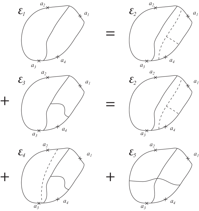
Figure 4: Self-duality decomposition

So one obtains eventually:

Proposition 1.

The scaling limit of the the expected number of clusters separating $a_{1}$ and $a_{4}$ from $a_{2}$ and $a_{3}$ is equal to:

$$\frac{2\pi\sqrt{3}}{\Gamma(\frac{1}{3})^{3}}\lambda^{\frac{1}{3}}\,\,{{}_{2}F_{1}}\left(\frac{1}{3},\frac{2}{3};\frac{4}{3};\lambda\right)-\frac{1}{2}\frac{\sqrt{3}}{2\pi}\lambda\,\,{{}_{3}F_{2}}\left(1,1,\frac{4}{3};\frac{5}{3},2;\lambda\right)+\frac{\sqrt{3}}{4\pi}\log\left(\frac{1}{1-\lambda}\right),$$

where the first term comes from Cardy’s formula, the second from Watts’ formula and the third from the main result of our paper.

3.3 Open questions

In this paper we show that certain observables have conformally invariant scaling limits. The most prominent mathematical tool for rigorous treatment of conformal invariance is Schramm’s $SLE$, which describes scaling limits of interfaces by the traces of the randomly driven Loewner evolutions – the so called $SLE_{\kappa}$ curves, see [8] for an introduction. Once convergence to $SLE$ is known, many quantities related to the model can be computed. The only proof for percolation uses Cardy’s formula for crossing probabilities (established for triangular lattice only in [10]) and locality of percolation or the so-called “martingale trick”, see [11, 12, 5].

3.3.1 How to use our observables to establish conformal invariance of critical percolation?

Whether our observable can replace the crossing probabilities in the proofs above, is interesting even if it has no less dependence on the triangular lattice. The problem that prevents the direct application of the same technique as in [12] is that our observable does not have a “martingale” property (see [13] for an overview) with respect to the percolation interface. However, one can attempt other approaches, for example exploiting locality.

3.3.2 Are our observables computable with $SLE$?

For the same reason, computing our observables with $SLE$ techniques (using this time that the percolation scaling limit is described by $SLE_{6}$) is not immediate. In principle, the computation should be possible, but the setup might be difficult.

3.3.3 Are there other similar observables?

Similar techniques allow to compute crossing probabilities and two similar observables in this paper. One can ask how much more one can learn without appealing to $SLE$ techniques, in particular whether there are any other computable observables?

4 Outline of the proof

The proof of Theorem 1 consists of three parts.

• First we prove that from each sequence $\left(H_{\delta_{n}}\right)_{n\in\mathbb{N}}$, with $\delta_{n}$ tending to $0$, one can extract a subsequence $H_{\delta_{k}}$ which converges uniformly on the compact subsets of $\bar{\Omega}\setminus\{l,r\}$ to a limit function $h$.

• We show then that any such subsequential limit $h$ satisfies the following boundary conditions:

  $$\mathrm{Im}(h) = \frac{\sqrt{3}}{4}\,\,\,\mbox{ on }u$$

  $$\mathrm{Im}(h) = -\frac{\sqrt{3}}{4}\,\,\,\mbox{ on }d$$

  $$\mathrm{Re}(h(w)) = 0$$

• We prove finally that $h$ is analytic.

In order to get that $h$ is the conformal map $\phi$ of Theorem 1, we observe that $h$ and $\phi$ have the same imaginary part (on the boundary and hence inside since the imaginary part is harmonic), and thus have the same real part up to a (real) constant by Cauchy-Riemann equations. The constant is $0$ since the real part of both is equal to $0$ at $w$. Since any subsequential limit has the desired value, we conclude by precompactness that $H_{\delta}$ converges to $\phi$.

5 Precompactness

In order to prove the precompactness of the family of functions $(H_{\delta})_{\delta>0}$, we show that the four families $(H_{\delta}^{l})_{\delta},(H_{\delta}^{r})_{\delta},(H_{\delta}^{u})_{\delta},(H_{\delta}^{d})_{\delta}$ are uniformly Hölder continuous on each compact subset of $\bar{\Omega}\setminus\{l,r\}$. Notice that since the interpolation is regular enough we may suppose in the estimates that the points we are considering are vertices of the hexagonal faces.

Lemma 1.

For every compact $K\subset\bar{\Omega}\setminus\{l,r\}$, the functions $H_{\delta}^{u}$ and $H_{\delta}^{d}$ are uniformly Hölder continuous on $K$ with respect to the metric $d$ of the length of the shortest path in $\bar{\Omega}$.

Proof.

We prove the result for $H_{\delta}^{u}$.

Let $\beta=\inf_{z\in K}\left(\max\left(\mathrm{dist}(z,u),\mathrm{dist}(z,d)\right)\right)$. By compactness of $K$ we have $\beta>0$, and so each point in $K$ is at distance at least $\beta$ from $u$ or $d$.

We have that for each $z,z^{\prime}\in\Omega$ the disc $D:=D((z+z^{\prime})/2,d(z,z^{\prime}))$ contains a path from $z$ to $z^{\prime}$.

Since $|H_{\delta}^{u}|$ is uniformly bounded, we can assume from now that the points $z$ and $z^{\prime}$ (in $K$) are close enough, i.e. such that $d(z,z^{\prime})\leq\beta$. By elementary partitioning we have that $|H_{\delta}^{u}(z)-H_{\delta}^{u}(z^{\prime})|\leq\mathbb{P}[Q_{\delta}^{u}(z)\setminus Q_{\delta}^{u}(z^{\prime})]+\mathbb{P}[Q_{\delta}^{u}(z^{\prime})\setminus Q_{\delta}^{u}(z)]$. So it is enough to show that there exists $C>0$ and $\alpha>0$ such that

$$\mathbb{P}[Q_{\delta}^{u}(z)\setminus Q_{\delta}^{u}(z^{\prime})]\leq C\cdot d(z,z^{\prime})^{\alpha}.$$

By self-duality, we have that the occurence of the event $Q_{\delta}^{u}(z)\setminus Q_{\delta}^{u}(z^{\prime})$ implies the connection of the boundary of the disc $D$ to $u$ by a black path and to $d$ by two disjoint white paths. Since at least one of the two sides is at distance $\beta$ (for $\delta$ sufficiently small, which we may suppose), this event implies the connection (by a black or white path) of a (microscopic) circle of radius $d(z,z^{\prime})$ to a circle of (macroscopic) radius $\beta$. By Russo-Seymour-Welsh Theorem (see [2], [7] for instance), there exists $C>0$ and $\alpha>0$ such that this event is of probability less that $C\cdot d(z,z^{\prime})^{\alpha}$ (uniformly in $\delta$) and this gives us the desired result. ∎

Lemma 2.

For every compact $K\subset\bar{\Omega}\setminus\{l,r\}$, the functions $H_{\delta}^{l}$ and $H_{\delta}^{r}$ are uniformly bounded and uniformly Hölder continuous on $K$ with respect the metric $d$ of the previous lemma.

Proof.

The proof is essentially the same as for the previous lemma: the probability that a cluster passes between two close points $z$ and $z^{\prime}$ is small (say $C(z,z^{\prime})$) for the same reasons. To control the expectation, we can use BK inequality which gives that the probability that $n$ disjoint clusters pass between $z$ and $z^{\prime}$ is smaller that $C(z,z^{\prime})^{n}$.

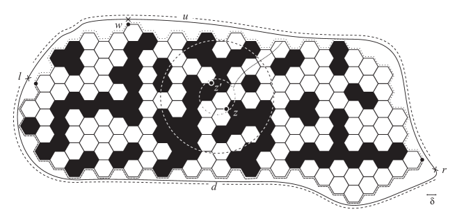
Figure 6: The event $\{N_{\delta}^{l}(z)=N_{\delta}^{l}(z^{\prime})+1\}$ implies a white connection of a microscopic circle of diameter $d(z,z^{\prime})$ to a macroscopic circle of diameter $\beta$ ($K$ is not fixed precisely on this picture).

∎

Proposition 2.

The function family $(H_{\delta})_{\delta>0}$ is precompact with respect to the topology of uniform convergence on every compact subset of $\bar{\Omega}\setminus\{l,r\}$.

Proof.

We are only interested in letting $\delta$ tend to $0$ (and otherwise it is anyway trivial). So let $\delta_{n}$ be a sequence tending to $0$. On each compact subset $K$ of $\bar{\Omega}\setminus\{l,r\}$, the functions $H_{\delta}^{l},H_{\delta}^{r},H_{\delta}^{u},H_{\delta}^{d}$ are bounded and uniformly Hölder continuous in $\delta$, so they form equicontinuous families. By Arzelà-Ascoli’s theorem, they form a precompact family. We can therefore extract a subsequence $\delta_{k}$ of $\delta_{n}$ such that $H_{\delta_{k}}^{l},H_{\delta_{k}}^{r},H_{\delta_{k}}^{u},H_{\delta_{k}}^{d}$ converge uniformly on $K$. Since $\bar{\Omega}\setminus\{l,r\}$ can be written as a countable union of compact subsets, a diagonal extraction gives us the desired result. ∎

6 Boundary conditions

Lemma 3.

We have the following boundary conditions:

$$\lim_{\delta\to 0}H_{\delta}^{u}(z)=0, \lim_{\delta\to 0}H_{\delta}^{d}(z)=\frac{1}{2},\quad\forall z\in u$$

$$\lim_{\delta\to 0}H_{\delta}^{u}(z)=\frac{1}{2}, \lim_{\delta\to 0}H_{\delta}^{d}(z)=0,\quad\forall z\in d$$

$$\lim_{\delta\to 0}H_{\delta}^{l}(w) = \lim_{\delta\to 0}H_{\delta}^{r}(w)=0$$

Proof.

By definition and continuity the condition for $H_{\delta}^{l}$ and $H_{\delta}^{r}$ is obvious.

For the first boundary value, notice that for $z$ on $u$, the event $Q_{\delta}^{u}(z)$ implies the connection of $z$ to $d$ (which is at a positive distance from $z$) by two white paths. By Russo-Seymour-Welsh, this probability tends to $0$ as $\delta\to 0$, so we are done.

For the second one, first notice that both $Q_{\delta}^{d}(z)$ and its color-negative $\tilde{Q_{\delta}^{d}}(z)$ cannot occur simultaneously for $z\in u$. By symmetry we obtain that $H_{\delta}^{d}(z)\leq\frac{1}{2}$. To see that the limit is actually $\frac{1}{2}$, it suffices because of the symmetry to prove that the probability that neither $Q_{\delta}^{d}(z)$ nor $\tilde{Q_{\delta}^{d}}(z)$ occur tends to $0$ as $\delta\to 0$.

Indeed if $Q_{\delta}^{d}(z)$ does not occur, then either there is no black path separating $z$ from $d$ (call this event $A$) or there is at least one black path separating $z$ from $d$ but these black paths do not touch $d$ (event $B$). By self-duality, $A$ is the event that $z$ is connected to $d$ by a white path. Again by self-duality, the occurence of $B$ implies that $\tilde{Q_{\delta}^{d}}(z)$ occurs: take the lowest black path $\gamma$ separating $z$ from $d$ (which does not touch $d$ by definition), so its lower boundary is a white path that touches $d$ (otherwise this white path would have a lower boundary which would be a black path and would thus contradict the definition of $\gamma$), which implies that $\tilde{Q_{\delta}^{d}}(z)$ occurs.

So if neither $Q_{\delta}^{d}(z)$ nor $\tilde{Q_{\delta}^{d}}(z)$ happen, $A$ happens. But as seen above, the probability of $A$ tends to $0$, since the probability of a connection by a white path from $z$ to $d$ tends to $0$ as $\delta\to 0$.

The arguments for $z\in d$ are the same as the ones for $z\in u$.

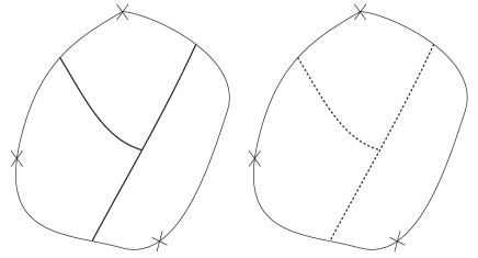
Figure 7: With probability tending to one as $\delta\to 0$, exactly one of these two events occurs.

∎

7 Analyticity

We are now interested in showing the analyticity of any subsequential limit of $H_{\delta}=(H_{\delta}^{l}+H_{\delta}^{r})-\frac{\sqrt{3}}{2}i(H_{\delta}^{u}-H_{\delta}^{d})$ as $\delta\to 0$ (since by Proposition 2 the family of functions $\left(H_{\delta}\right)_{\delta>0}$ is precompact). The main step consists in proving that for each $\delta>0$, the function $H_{\delta}$ is discrete analytic in a sense explained in the next paragraph, which allows to show that Morera’s condition is satisfied.

7.1 Discrete Cauchy-Riemann equations

Let us first introduce several notations.

For an oriented edge $\vec{e}=\langle x,y\rangle$ in the interior of $\Omega_{\delta}$, let us denote by $\vec{\tau.e}$ and $\vec{\tau^{2}.e}$ the edges of $\Omega_{\delta}$ obtained by rotating counterclockwise $\vec{e}$ around $x$ by an angle of $2\pi/3$ and $4\pi/3$ respectively. We will denote by $\vec{e^{*}}$ the dual edge of $\vec{e}$: the edge from the center of the hexagon on the right of $\vec{e}$ to the center of the hexagon on the left of $\vec{e}$.

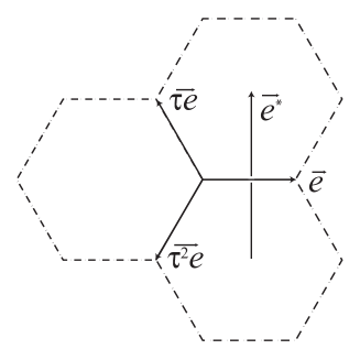
Figure 8: Edges notations

For a function $F$ defined on the set of vertices of $\Omega_{\delta}$ and an oriented edge $\vec{e}=\langle x,y\rangle$, let us define $\partial_{\vec{e}}F$ as $F(y)-F(x)$.

Let $\partial_{\vec{e}}^{\pm}H_{\delta}^{l}$ be $\mathbb{P}[N_{\delta}^{l}(y)=N_{\delta}^{l}(x)\pm 1]$ By linearity of the expectation it is easy to see that $\partial_{\vec{e}}H_{\delta}^{l}=\partial_{\vec{e}}^{+}H_{\delta}^{l}-\partial_{\vec{e}}^{-}H_{\delta}^{l}$. Let $\partial_{\vec{e}}^{+}H_{\delta}^{u}$ be $\mathbb{P}[Q_{\delta}^{u}(y)\setminus Q_{\delta}^{u}(x)]$ and $\partial_{\vec{e}}^{-}H_{\delta}^{u}$ be $\partial_{-\vec{e}}^{+}H_{\delta}^{u}=\mathbb{P}[Q_{\delta}^{u}(x)\setminus Q_{\delta}^{u}(y)]$. As before we have $\partial_{\vec{e}}H_{\delta}^{u}=\partial_{\vec{e}}^{+}H_{\delta}^{u}-\partial_{\vec{e}}^{-}H_{\delta}^{u}$.

For $H_{\delta}^{r}$ and $H_{\delta}^{d}$, we define $\partial_{\vec{e}}^{+}$ and $\partial_{\vec{e}}^{-}$ in the same way as for $H_{\delta}^{l}$ and $H_{\delta}^{u}$ respectively and also obtain $\partial_{\vec{e}}=\partial_{\vec{e}}^{+}-\partial_{\vec{e}}^{-}$. By linearity it is also defined for $H_{\delta}$.

We have the following discrete analyticity result, which already suggests that $H_{\delta}$ is analytic in the limit and is a discrete analogue of the Cauchy-Riemann equations.

Proposition 3 (Discrete Cauchy-Riemann equations).

For any $\delta>0$ and any oriented edge $\vec{e}$ in the interior of $\Omega_{\delta}$, we have the following identity:

$$2\left(\partial_{\vec{e}}^{+}H_{\delta}^{l}-\partial_{\vec{e}}^{-}H_{\delta}^{r}-\right)=\left(\partial_{\vec{\tau.e}}^{+}-\partial_{\vec{\tau^{2}.e}}^{+}\right)\left(H_{\delta}^{d}-H_{\delta}^{u}\right)$$

Proof.

Notice that since each configuration (coloring of the hexagons) has equal probability, bijective maps are measure-preserving. We will use this fact several times in the proof. Fix $\delta>0$, take as before $\vec{e}=\langle x,y\rangle$ and introduce the following notations.

In what follows, $\tau.y$ and $\tau^{2}.y$ will be the vertices of $\Omega_{\delta}$ such that $\vec{\tau.e}=\langle x,\tau y\rangle$ and $\vec{\tau^{2}.e}=\langle x,\tau^{2}y\rangle$. Let $\mathcal{L}$ (respectively $\mathcal{R}$ ; $\mathcal{I}$ ; $\mathcal{T}$) be the hexagonal face that is adjacent to $\vec{e}$ and $\vec{\tau^{2}.e}$ (respectively to $\vec{e}$ and $\vec{\tau.e}$ ; to $\vec{\tau.e}$ and $\vec{\tau^{2}.e}$ ; the hexagon that touches $y$). For a hexagonal face, for instance $\mathcal{L}$, we denote by $\mathcal{L}_{w}$ the event that this face is connected by a white path to $d$, by $\mathcal{L}^{b}$ the event that it is connected by a black path to $u$, by $\mathcal{L}_{w}^{w}$ the event that it is connected by (not necessarily disjoint) white paths to both $u$ and $d$, and etc.: the connections to $u$ are denoted by superscripts, the connections to $d$ by subscripts. Recall that we use the notation $A\circ B$ for the event that both $A$ and $B$ occur on disjoint sites (notice that it is well defined for the events we use here).

We now compute the derivative $\partial_{\vec{e}}^{-}$ of $H_{\delta}^{r}$. We have that the event $A:=\{N_{\delta}^{r}(x)=N_{\delta}^{r}(y)+1\}$ is the same as $B:=\mathcal{I}_{b}^{b}\circ\mathcal{L}_{w}\circ R^{w}$, since it is clear that $B$ implies $A$, and by self-duality, if $B$ does not occur, then $A$ does not occur (since otherwise there would be a white path touching the right boundary of the white cluster passing between $y$ and $x$ and separating $x$ from $r$ which would be absurd by definition of the right boundary), so both are equal.

Notice that on this event, by going from $y$ to $x$, either we gain a cluster boundary counting positively or we lose a cluster boundary counting negatively.

If $B$ occurs, then we can define $\lambda$ as the counterclockwise-most extremal white path that joins $\mathcal{L}$ to $d$ (call $\lambda_{d}$ its hexagon on $d$) and $\rho$ as the clockwise-most extremal white path that joins $\mathcal{R}$ to $u$ (call $\rho_{u}$ its hexagon on $u$). We can then us a self-duality argument in the interior of rectangle $l,\lambda_{d},\mathcal{T},\rho_{u}$ (we consider the topological rectangle delimited by $\lambda$ (excluded), $\rho$ (excluded), the arc $\rho_{u}l$ (included) and the arc $l\lambda_{d}$ (included)): $B$ is the disjoint union of $C$ and $D$, where $C$ is the event that $B$ happens and that there is a white path that joins the arcs $l\lambda_{d}$ and $\mathcal{T}\rho_{u}$ and $D$ is the event that $B$ happens and that there is a black path that joins the arcs $\rho_{u}l$ and $\lambda_{d}\mathcal{T}$ (these events occur in the interior of the rectangle). So we have $\mathbb{P}[B]=\mathbb{P}[C]+\mathbb{P}[D]$. But $C$ is equal to $\mathcal{I}_{b}^{b}\circ\mathcal{L}_{w}\circ\mathcal{R}_{w}^{w}$ and we have that $D$ and $\mathcal{I}_{b}^{b}\circ\mathcal{L}_{w}^{w}\circ\mathcal{R}^{w}$ are clearly in bijection: it suffices to flip (i.e. invert) the colors inside the rectangle to map one onto the other (this is well-defined because the definition of the rectangle does not depend on the colors of the hexagons inside), and so the configuration inside is independent of the colors elsewhere.

But now we have that $\mathcal{I}_{b}^{b}\circ\mathcal{L}_{w}\circ\mathcal{R}_{w}^{w}$ and $\mathcal{I}_{w}^{w}\circ\mathcal{L}_{b}\circ\mathcal{R}_{w}^{w}$ also have the same probability. Let $\iota$ be the clockwise-most extremal black path that joins $\mathcal{I}$ to $u$, and flip the colors in the interior of the part of the graph $G$ comprised between $\iota$ and $\lambda$ that contains $l$ ($\iota$ and $\lambda$ excluded). Then flip all the colors of $\Omega_{\delta}$. This defines a (clearly bijective) map from $\mathcal{I}_{b}^{b}\circ\mathcal{L}_{w}\circ\mathcal{R}_{w}^{w}$ to $\mathcal{I}_{w}^{w}\circ\mathcal{L}_{b}\circ\mathcal{R}_{w}^{w}$. The same color-flipping argument shows that $\mathcal{I}_{b}^{b}\circ\mathcal{L}_{w}^{w}\circ\mathcal{R}^{w}$ and $\mathcal{I}_{w}^{w}\circ\mathcal{L}_{w}^{w}\circ\mathcal{R}^{b}$ also have the same probability. So we can summarize the discussion above in the following equations, see Figure 10:

$$\partial_{\vec{e}}^{-}H_{\delta}^{r} = \mathbb{P}[N_{\delta}^{r}(x)=N_{\delta}^{r}(y)+1]$$

$$= \mathbb{P}[\mathcal{I}_{b}^{b}\circ\mathcal{L}_{w}\circ\mathcal{R}^{w}]$$

$$= \mathbb{P}[\mathcal{I}_{b}^{b}\circ\mathcal{L}_{w}\circ\mathcal{R}_{w}^{w}]+\mathbb{P}[\mathcal{I}_{b}^{b}\circ\mathcal{L}_{w}^{w}\circ\mathcal{R}^{w}]$$

$$= \mathbb{P}[\mathcal{I}_{w}^{w}\circ\mathcal{L}_{b}\circ\mathcal{R}_{w}^{w}]+\mathbb{P}[\mathcal{I}_{w}^{w}\circ\mathcal{L}_{w}^{w}\circ\mathcal{R}^{b}].$$

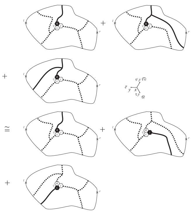
Figure 11: Computation of $\partial_{\vec{\tau.e}}^{+}H_{\delta}^{u}$.

Using a very similar method (but considering this time a rectangle that contains $r$ instead of $l$ when applying self-duality), one obtains, see Figure 11:

$$\partial_{\vec{e}}^{+}H_{\delta}^{l} = \mathbb{P}[N_{\delta}^{l}(y)=N_{\delta}^{l}(x)+1]$$

$$= \mathbb{P}[\mathcal{I}_{b}^{b}\circ\mathcal{L}^{w}\circ\mathcal{R}_{w}]$$

$$= \mathbb{P}[\mathcal{I}_{b}^{b}\circ\mathcal{L}_{w}^{w}\circ\mathcal{R}_{w}]+\mathbb{P}[\mathcal{I}_{b}^{b}\circ\mathcal{L}^{b}\circ\mathcal{R}_{w}^{w}]$$

$$= \mathbb{P}[\mathcal{I}_{w}^{w}\circ\mathcal{L}_{w}^{w}\circ\mathcal{R}_{b}]+\mathbb{P}[\mathcal{I}_{w}^{w}\circ\mathcal{L}^{b}\circ\mathcal{R}_{w}^{w}]$$

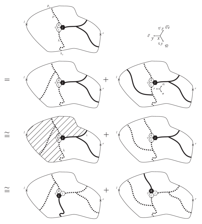
Figure 9: Computation of $\partial_{\vec{e}}^{-}H_{\delta}^{r}$. White paths are dashed and black path bold. The stripped region is $G$ (the subgraph where the color are flipped).

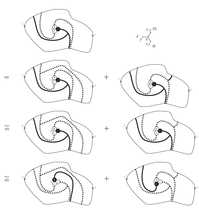
Figure 10: Computation of $\partial_{\vec{e}}^{+}H_{\delta}^{l}$.

Let us now compute the derivative $\partial_{\vec{\tau.e}}^{+}$ of $H_{\delta}^{u}$. By self-duality we have that the event $X:=Q_{\delta}^{u}(\tau.y)\setminus Q_{\delta}^{u}(x)$ is the same as the event that $\mathcal{I}$ and $\mathcal{L}$ are on a white simple path from $d$ to $d$ which is connected to $u$. $\mathcal{R}$ is connected by a black path to $u$ (otherwise there would be a white path separating it from $u$ and this path would be connected by a white path to $u$ as well because $Q_{\delta}^{u}(\tau.y)$ occurs, which would imply that $Q_{\delta}^{u}(x)$ also occurs). Suppose that $X$ occurs. Let $\lambda^{\prime}$ be the clockwise-most extremal white path that joins $\mathcal{L}$ to $d$ and $\iota^{\prime}$ the counterclockwise-most extremal white path that joins $\mathcal{I}$ to $d$. Then obviously, exactly one of the three following events occurs:

1. $Y:=\mathcal{I}_{w}^{w}\circ\mathcal{L}_{w}^{w}\circ\mathcal{R}^{b}$: there is a white path that joins $\lambda^{\prime}$ to $u$ and there is a white path that joins $\iota^{\prime}$ to $u$.

2. $Z:=\mathcal{I}_{w}^{w}\circ\mathcal{L}_{w}\circ\mathcal{R}_{b}^{b}$: there is a white path that joins $\lambda^{\prime}$ to $u$ and there is no white path that joins $\iota^{\prime}$ to $u$.

3. $W:=\mathcal{I}_{w}\circ\mathcal{L}_{w}^{w}\circ\mathcal{R}_{b}^{b}$: there is no white path that joins $\lambda^{\prime}$ to $u$ and there is a white path that joins $\iota^{\prime}$ to $u$.

Using a color-flipping argument we obtain that $\mathbb{P}[Z]=\mathbb{P}[\mathcal{I}_{w}^{w}\circ\mathcal{L}_{b}\circ\mathcal{R}_{w}^{w}]$: take the counterclockwise-most black path that joins $\mathcal{R}$ to $u$, call it $\gamma_{1}$, the clockwise-most white path that joins $\mathcal{L}$ to $d$, call it $\gamma_{2}$, flip the colors in the interior of the part of $\Omega_{\delta}$ delimited by $\gamma_{1}$ and $\gamma_{2}$ that contains $r$ ($\gamma_{1}$ and $\gamma_{2}$ excluded), then flip the colors of the whole graph. This defines a bijection from $Z$ to $\mathcal{I}_{w}^{w}\circ\mathcal{L}_{b}\circ\mathcal{R}_{w}^{w}$. Thus we have shown that

$$\partial_{\vec{\tau.e}}^{+}H_{\delta}^{u} = \mathbb{P}[\mathcal{I}_{w}^{w}\circ\mathcal{L}_{w}^{w}\circ\mathcal{R}^{b}]+\mathbb{P}[\mathcal{I}_{w}^{w}\circ\mathcal{L}_{b}\circ\mathcal{R}_{w}^{w}]+\mathbb{P}[\mathcal{I}_{b}\circ\mathcal{L}_{w}^{w}\circ\mathcal{R}_{w}^{w}].$$

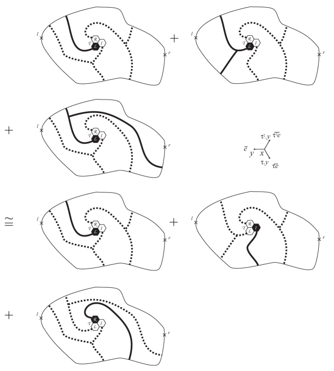
Figure 13: Computation of $\partial_{\vec{\tau^{2}.e}}^{+}H_{\delta}^{u}$.

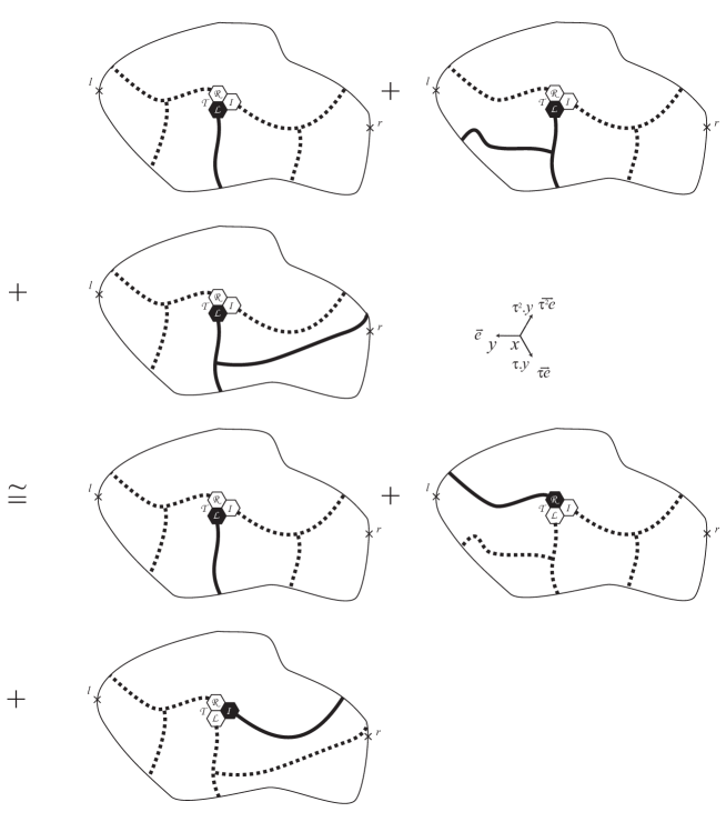
Figure 14: Computation of $\partial_{\vec{\tau^{2}.e}}^{+}H_{\delta}^{d}$.

One obtains similarly, see Figures 13-15 at the end of the section:

$$\partial_{\vec{\tau.e}}^{+}H_{\delta}^{d} = \mathbb{P}[\mathcal{I}_{w}^{w}\circ\mathcal{L}^{b}\circ\mathcal{R}_{w}^{w}]+\mathbb{P}[\mathcal{I}_{w}^{w}\circ\mathcal{L}_{w}^{w}\circ\mathcal{R}_{b}]+\mathbb{P}[\mathcal{I}_{b}\circ\mathcal{L}_{w}^{w}\circ\mathcal{R}_{w}^{w}]$$

$$\partial_{\vec{\tau^{2}.e}}^{+}H_{\delta}^{u} = \mathbb{P}[\mathcal{I}_{w}^{w}\circ\mathcal{L}_{w}^{w}\circ\mathcal{R}_{b}]+\mathbb{P}[\mathcal{I}_{w}^{w}\circ\mathcal{L}^{b}\circ\mathcal{R}_{w}^{w}]+\mathbb{P}[\mathcal{I}^{b}\circ\mathcal{L}_{w}^{w}\circ\mathcal{R}_{w}^{w}]$$

$$\partial_{\vec{\tau^{2}.e}}^{+}H_{\delta}^{d} = \mathbb{P}[\mathcal{I}_{w}^{w}\circ\mathcal{L}_{b}\circ\mathcal{R}_{w}^{w}]+\mathbb{P}[\mathcal{I}_{w}^{w}\circ\mathcal{L}_{w}^{w}\circ\mathcal{R}^{b}]+\mathbb{P}[\mathcal{I}^{b}\circ\mathcal{L}_{w}^{w}\circ\mathcal{R}_{w}^{w}]$$

Summing up the identities obtained so far, we obtain the desired result. ∎

7.2 Morera’s condition

The last step in order to prove the analyticity of $h$ is to show that any contour integral of the subsequential limit $h$ vanishes. This is given by the following proposition (since the convergence is uniform on each compact subset of $\Omega$, the integral is equal to the limit of the integrals $\oint_{\gamma}H_{\delta}(z)\,\mathrm{d}z$ as $\delta\to 0$).

Proposition 4 (Morera’s condition for $h$).

Let $\gamma$ be a simple closed smooth curve in $\Omega$ oriented counterclockwise. Then we have

$$\oint_{\gamma}H_{\delta}(z)\,\mathrm{d}z\to 0\quad\mbox{as $\delta\to 0$}$$

Proof.

For each sufficiently small $\delta>0$, let $\gamma_{\delta}$ be a discretization of $\gamma$, such that $\gamma_{\delta}$ is a simple curve oriented in the same direction consisting in edges that follow the orientation of $\gamma_{\delta}$ and such that $\gamma_{\delta}\to\gamma$ as $\delta\to 0$ in the Hausdorff metric and with a number of edges of order $\delta^{-1}$.

For $\vec{e}=\langle x,y\rangle$, let us define $F(\vec{e}):=\frac{F(x)+F(y)}{2}$ and $\vec{e}=y-x$ (when appears alone). We approximate the integral $\oint_{\gamma}H_{\delta}(z)\,\mathrm{d}z$ by a Riemann sum along $\gamma_{\delta}$ defined as $\sum_{\vec{e}\in\gamma}\vec{e}H_{\delta}(\vec{e})$.

As $\delta\to 0$, one has $\left|\oint_{\gamma}H_{\delta}(z)\,\mathrm{d}z-\sum_{\vec{e}\in\gamma}\vec{e}H_{\delta}(\vec{e})\right|\to 0$, by precompactness of the family $\left(H_{\delta}\right)_{\delta>0}$ in the topology of uniform convergence on the compact subsets.

We now use the following discrete summation lemma (cf. [1]). Define $\mathrm{Int}(\gamma_{\delta})$ as the set of all oriented edges lying in the interior of the part of $\Omega_{\delta}$ which is inside $\gamma_{\delta}$ and recall that $\vec{e^{*}}$ is the dual edge of $\vec{e}$ (seen as a scalar it is equal to $\sqrt{3}i\vec{e}$).

Lemma 4.

$$\sum_{\vec{e}\in\gamma_{\delta}}\vec{e}H_{\delta}(\vec{e})=\sum_{\vec{e}\in\mathrm{Int}(\gamma_{\delta})}\vec{e^{*}}\partial_{\vec{e}}^{+}H_{\delta}+o_{\delta\to 0}(1)$$

Proof.

Denote by $\mathrm{Hex}(\gamma_{\delta})$ the set of hexagonal faces of $\Omega_{\delta}$ which are inside $\gamma_{\delta}$ and for such a face $f$, denote by $\partial f$ the set of its six edges oriented in counterclockwise direction. We have that

$$\sum_{\vec{e}\in\gamma_{\delta}}\vec{e}H_{\delta}(\vec{e})=\sum_{f\in\mathrm{Hex}(\gamma_{\delta})}\sum_{f\in\partial f}\vec{e}H_{\delta}(\vec{e}),$$

since the terms appearing in edges that are not on $\gamma_{\delta}$ appear twice (in two faces to which such an edge belongs) with opposite signs and therefore cancel. Denote by $\langle x_{0},x_{1}\rangle,\langle x_{1},x_{2}\rangle,\ldots,\langle x_{5},x_{0}\rangle$ the six edges of $\partial f$ and take the indices modulo $6$; denote by $c(f)$ the center of a hexagonal face (this term is purely artificial yet). A simple calculation shows:

$$\sum_{\vec{e}\in\partial f}\vec{e}H_{\delta}(\vec{e})=\sum_{k=0}^{5}\left(\frac{x_{k}+x_{k+1}}{2}-c(f)\right)(H(x_{k+1})-H(x_{k})).$$

If $\langle x_{k},x_{k}+1\rangle$ does not lie on $\gamma_{\delta}$, the term $\frac{x_{k}+x_{k+1}}{2}(H(x_{k+1})-H(x_{k}))$ appears twice with opposite signs and cancels, so only the terms with the factor $c(f)$ remain. A term of the form $H(x_{k+1})-H(x_{k})$ becomes a factor of the difference between two center faces which is the edge dual to $\langle x_{k},x_{k+1}\rangle$.

On the other hand, we have that the contribution of the boundary terms on $\gamma_{\delta}$ tends to $0$: we have that the number of edges of $\gamma_{\delta}$ is of order $\delta^{-1}$, the term $\frac{x_{k}+x_{k+1}}{2}-c(f)$ is of order $\delta$ and $H_{\delta}$ is Hölder on a neighborhood of $\gamma$.

We obtain that the sum is equal to

$$\sum_{\vec{e}\in\mbox{CcwInt}(\gamma_{\delta})}\vec{e^{*}}\partial_{\vec{e}}H_{\delta}+o(1),\quad\mbox{as $\delta\to 0$}$$

where CcwInt is the set of the counterclockwise oriented edges of the set of faces $\mathrm{Hex}(\gamma_{\delta})$. Taking the sum over the set $\mathrm{Int}(\gamma_{\delta})$ of all oriented edges inside $\gamma_{\delta}$, using $\partial_{\vec{e}}=\partial_{\vec{e}}^{+}-\partial_{-\vec{e}}^{+}$, we obtain

$$\sum_{\vec{e}\in\mathrm{Int}(\gamma_{\delta})}\vec{e^{*}}\partial_{\vec{e}}^{+}H_{\delta}+o(1),\quad\mbox{as $\delta\to 0$}$$

as required.

∎

Now it suffices to prove that the sum $\sum_{\vec{e}\in\mathrm{Int}(\gamma_{\delta})}\vec{e^{*}}\partial_{\vec{e}}^{+}H_{\delta}$ given by the previous lemma is equal to $0$. This is given by the discrete Cauchy-Riemann equations. Let us reorder the terms in the sum in the following way:

$$\sum_{\vec{e}\in\mathrm{Int}(\gamma_{\delta})}\vec{e^{*}}\partial_{\vec{e}}^{+}H_{\delta} = \sum_{\vec{e}\in\mathrm{Int}(\gamma_{\delta})}\vec{e^{*}}\partial_{\vec{e}}^{+}\left(H_{\delta}^{r}+H_{\delta}^{l}-\frac{\sqrt{3}}{2}i(H_{\delta}^{u}-H_{\delta}^{d})\right)$$

$$= -\sum_{\vec{e}\in\mathrm{Int}(\gamma_{\delta})}\vec{e^{*}}\left(\partial_{\vec{e}}^{-}H_{\delta}^{r}-\partial_{\vec{e}}^{+}H_{\delta}^{l}+\frac{\sqrt{3}}{2}i\partial_{\vec{e}}^{+}(H_{\delta}^{u}-H_{\delta}^{d})\right)$$

$$= -\sum_{\vec{e}\in\mathrm{Int}(\gamma_{\delta})}\vec{e^{*}}\left(\frac{\partial_{\vec{\tau.e}}^{+}H_{\delta}^{u}-\partial_{\vec{\tau.e}}^{+}H_{\delta}^{d}-\partial_{\vec{\tau^{2}.e}}^{+}H_{\delta}^{u}+\partial_{\vec{\tau^{2}.e}}^{-}H_{\delta}^{d}}{2}\right.$$

$$\left.+\frac{\sqrt{3}}{2}i\partial_{\vec{e}}^{+}(H_{\delta}^{u}-H_{\delta}^{d})\right),$$

where last equality is obtained using the discrete Cauchy-Riemann equations. Reordering one last time the sum (using the changes of variables $\vec{(\tau.e)^{*}}\to\vec{e^{*}}$ and $\vec{(\tau^{2}.e)^{*}}\to\vec{e^{*}}$ in the first and the second parts of the sum respectively), we obtain

$$-\frac{1}{2}\sum_{\vec{e}\in\mathrm{Int}(\gamma_{\delta})}\left(\sqrt{3}i\vec{e^{*}}+(\vec{(\tau^{2}.e)^{*}}-\vec{(\tau.e)^{*}})\right)\partial_{\vec{e}}^{+}(H_{\delta}^{u}-H_{\delta}^{d}),$$

which is equal to $0$, since $\left(\sqrt{3}i\vec{e^{*}}+(\vec{(\tau^{2}.e)^{*}}-\vec{(\tau.e)^{*}})\right)=0$ by the geometry of the lattice (and this is in fact the only step in our proof where the actual embedding of the lattice is crucial).

∎

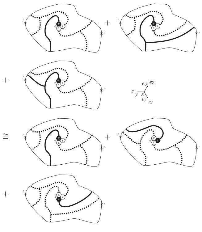
Figure 12: Computation of $\partial_{\vec{\tau.e}}^{+}H_{\delta}^{d}$.

References

- [1] V. Beffara, Cardy’s formula on the triangular lattice, the easy way, in Universality and renormalization, 39–45, Fields Inst. Commun., 50, Amer. Math. Soc., Providence, RI, 2007.
- [2] B. Bollobas, O. Riordan, Percolation, Cambridge University Press, 2006.
- [3] J. Cardy, Critical percolation in finite geometries, J. Phys. A, 25:L201–206, 1992.
- [4] J. Cardy, Conformal Invariance and Percolation, arXiv:math-ph/0103018.
- [5] F. Camia, C. Newman, Critical percolation exploration path and SLE 6: a proof of convergence, Probability Theory and Related Fields, 139, (3), 473–519, 2007.
- [6] J. Dubédat, Excursion decompositions for SLE and Watts’ crossing formula, Probab. Theory Related Fields, 2006, no. 3, 453–488.
- [7] G. Grimmett, Percolation, Springer-Verlag, 1999.
- [8] G. F. Lawler, Conformally Invariant Processes in the Plane, volume 114. Mathematical Surveys and Monographs, 2005.
- [9] J. H. Simmons, P. Kleban, R. M. Ziff, Percolation crossing formulae and conformal field theory, J. Phys. A 40 (2007), no. 31, F771–F784.
- [10] S. Smirnov, Critical percolation in the plane: Conformal invariance, Cardy’s formula, scaling limits, C. R. Acad. Sci. Paris Sr. I Math. 333 (2001), 239–244.
- [11] S. Smirnov, Critical percolation in the plane, preprint, 2001.
- [12] S. Smirnov, Critical percolation and conformal invariance, XIVth International Congress on Mathematical Physics (Lissbon, 2003), 99–112, World Sci. Publ., Hackensack, NJ.
- [13] S. Smirnov, Towards conformal invariance of 2D lattice models, Sanz-Sole, Marta (ed.) et al., Proceedings of the international congress of mathematicians (ICM), Madrid, Spain, August 22-30, 2006. Volume II: Invited lectures, 1421–1451. Zurich: European Mathematical Society (EMS), 2006.
- [14] S. Smirnov, W. Werner, Critical exponents for two-dimensional percolation, Math. Research Letters 8 (2001), no. 5–6, 729–744, 2001.
- [15] G.M.T. Watts. A crossing probability for critical percolation in two dimensions, J. Phys. A29:L363, 1996.