Determination of Low Energy Constants and testing Chiral Perturbation Theory at order $p^{6}$ (NNLO)

Johan Bijnens
Department of Theoretical Physics, Lund University, Sรถlvegatan 14A, SE 22362 Lund, Sweden
E-mail
bijnens@thep.lu.se
โ€ƒโ€ƒ
Department of Theoretical Physics, Lund University, Sรถlvegatan 14A, SE 22362 Lund, Sweden
E-mail
Abstract:

We present the results of a search for relations between observables that are independent of the Chiral Perturbation Theory (ChPT) Next-to-Next-to-Leading Order (NNLO) Low-Energy Constants (LECs). We have found some relations between observables in $\pi\pi$, $\pi K$ scattering and $K_{l4}$ decay which have been evaluated numerically using fit 10 inย [1] for the NLO LECs. We also show some preliminary results for a new global fit of the NLO LECs

1 Introduction

Testing the validity of Chiral Perturbation Theory (ChPT) is a challenging task because of the many unknown parameters, called the Low Energy Constants (LECs), entering into the theory. In particular, at NNLO $90$ unknown constants, the $C_{i}$, appear in the $p^{6}$ Lagrangian.

One way to overcome this problem is to study different combinations of observables that depend on the $C_{i}$ in the same way. These lead to $C_{i}$-independent relations which can be used to perform the test. Furthermore those combinations might be useful to gain information on the LECs too, since they let us isolate the same combinations of $C_{i}$ using different observables.

Inย [2] we study $76$ observables at NNLO and find $36$ such relations. We compare ChPT NNLO predictions with data/dispersive results for $13$ of these. The observables involved are the ones in $\pi\pi$ and $\pi K$-scattering and in $K_{\ell 4}$ decay. Here we first discuss how we perform the numerical analysis, the results of which appear in Tab.1, 2, 3 and 4, then we present for each process the relations studied. Finally we show some preliminary results for a new global fit of the $L_{i}$ at NNLO.

2 Numerical Analysis

The numerical analysis of the $C_{i}$-independent relations has been done in the following way. First we evaluate the combinations of observables appearing in each side of the relations using experiment/dispersive (exp) results ofย [3] for $\pi\pi$ scattering,ย [4] for $\pi K$ scattering andย [5, 6] for $K_{\ell 4}$ decay. Then we use ChPT results up to order $p^{6}$ [7, 8, 9] setting the $L_{i}$ to the values of fit 10 inย [1]. Finally we subtract from the first (exp) evaluation the ChPT one. These differences will contain the $C_{i}$ part and higher order corrections. They have been quoted in Tab.1, 2, 3 and 4 in the columns labeled remainder. This has been done for each side of the relations under study. To check whether a relation is well satisfied we compare the remainders of its left-hand-side (LHS) and right-hand-side (RHS). Since they contain the same $C_{i}$ combinations, they should be equal within the uncertainties.

The errors quoted in the second columns of Tab.1, 2, 3 and 4 are obtained adding in quadrature the uncertainties in ย [3, 4, 5, 6]. This might result in an underestimate of the total error because of correlations. The theoretical errors due to the NLO LECs are shown in brackets in the columns of Tab.1, 2, 3 and 4 labeled NNLO 1-loop. They are obtained by varying all the $L_{i}$ around the central values of fit 10 according to the full covariance matrix as obtained by the authors ofย [1] and exploring the region with $\chi^{2}/\textrm{dof}\approx 1$ . The error is then estimated as the maximum deviation observed. The error for the $L_{i}$ contribution at NLO is never shown since it drops out of all the relations. No uncertainties due to higher order contributions have been added. The uncertainties due to theoretical errors are mostly on the last quoted digit.

3 $\pi\pi$ scattering

The $\pi\pi$ scattering amplitude can be written as a function Aโ€‹(s,t,u)๐ด๐‘ ๐‘ก๐‘ขA(s,t,u) which is symmetric in $t,\,u$:

Aโ€‹(ฯ€aโ€‹ฯ€bโ†’ฯ€cโ€‹ฯ€d)=ฮดa,bโ€‹ฮดc,dโ€‹Aโ€‹(s,t,u)+ฮดc,dโ€‹ฮดb,dโ€‹Aโ€‹(t,u,s)+ฮดa,dโ€‹ฮดb,cโ€‹Aโ€‹(u,t,s),๐ดโ†’superscript๐œ‹๐‘Žsuperscript๐œ‹๐‘superscript๐œ‹๐‘superscript๐œ‹๐‘‘superscript๐›ฟ๐‘Ž๐‘superscript๐›ฟ๐‘๐‘‘๐ด๐‘ ๐‘ก๐‘ขsuperscript๐›ฟ๐‘๐‘‘superscript๐›ฟ๐‘๐‘‘๐ด๐‘ก๐‘ข๐‘ superscript๐›ฟ๐‘Ž๐‘‘superscript๐›ฟ๐‘๐‘๐ด๐‘ข๐‘ก๐‘ A(\pi^{a}\pi^{b}\rightarrow\pi^{c}\pi^{d})=\delta^{a,b}\delta^{c,d}A(s,t,u)+\delta^{c,d}\delta^{b,d}A(t,u,s)+\delta^{a,d}\delta^{b,c}A(u,t,s)\,, (1)

where s,t,u๐‘ ๐‘ก๐‘ขs,t,u are the usual Mandelstam variables. The isospin amplitudes TIโ€‹(s,t)superscript๐‘‡๐ผ๐‘ ๐‘กT^{I}(s,t) $(I=0,1,2)$ are T0โ€‹(s,t)=3โ€‹Aโ€‹(s,t,u)+Aโ€‹(t,u,s)+Aโ€‹(u,s,t),T1โ€‹(s,t)=Aโ€‹(s,t,u)โˆ’Aโ€‹(u,s,t),T2โ€‹(s,t)=Aโ€‹(t,u,s)+Aโ€‹(u,s,t),formulae-sequencesuperscript๐‘‡0๐‘ ๐‘ก3๐ด๐‘ ๐‘ก๐‘ข๐ด๐‘ก๐‘ข๐‘ ๐ด๐‘ข๐‘ ๐‘กformulae-sequencesuperscript๐‘‡1๐‘ ๐‘ก๐ด๐‘ ๐‘ก๐‘ข๐ด๐‘ข๐‘ ๐‘กsuperscript๐‘‡2๐‘ ๐‘ก๐ด๐‘ก๐‘ข๐‘ ๐ด๐‘ข๐‘ ๐‘กT^{0}(s,t)=3A(s,t,u)+A(t,u,s)+A(u,s,t)\,,\,T^{1}(s,t)=A(s,t,u)-A(u,s,t)\,,\,T^{2}(s,t)=A(t,u,s)+A(u,s,t)\,,\, and are expanded in partial waves

TIโ€‹(s,t)superscript๐‘‡๐ผ๐‘ ๐‘ก\displaystyle T^{I}(s,t) $\displaystyle=$ 32โ€‹ฯ€โ€‹โˆ‘โ„“=0+โˆž(2โ€‹โ„“+1)โ€‹Pโ„“โ€‹(cosโกฮธ)โ€‹tโ„“Iโ€‹(s),32๐œ‹superscriptsubscriptโ„“02โ„“1subscript๐‘ƒโ„“๐œƒsuperscriptsubscript๐‘กโ„“๐ผ๐‘ \displaystyle 32\pi\sum_{\ell=0}^{+\infty}(2\ell+1)P_{\ell}(\cos{\theta})t_{\ell}^{I}(s), (2)

where $t$ and $u$ have been written as t=โˆ’12โ€‹(sโˆ’4โ€‹mฯ€2)โ€‹(1โˆ’cosโกฮธ)๐‘ก12๐‘ 4subscriptsuperscript๐‘š2๐œ‹1๐œƒt=-\frac{1}{2}(s-4m^{2}_{\pi})(1-\cos{\theta}), u=โˆ’12โ€‹(sโˆ’4โ€‹mฯ€2)โ€‹(1+cosโกฮธ)๐‘ข12๐‘ 4subscriptsuperscript๐‘š2๐œ‹1๐œƒu=-\frac{1}{2}(s-4m^{2}_{\pi})(1+\cos{\theta}). Near threshold the $t^{I}_{\ell}$ are further expanded in terms of the threshold parameters

tโ„“Iโ€‹(s)=q2โ€‹โ„“โ€‹(aโ„“I+bโ„“Iโ€‹q2+๐’ชโ€‹(q4)),q2=14โ€‹(sโˆ’4โ€‹mฯ€2),formulae-sequencesuperscriptsubscript๐‘กโ„“๐ผ๐‘ superscript๐‘ž2โ„“superscriptsubscript๐‘Žโ„“๐ผsuperscriptsubscript๐‘โ„“๐ผsuperscript๐‘ž2๐’ชsuperscript๐‘ž4superscript๐‘ž214๐‘ 4subscriptsuperscript๐‘š2๐œ‹\displaystyle t_{\ell}^{I}(s)=q^{2\ell}(a_{\ell}^{I}+b_{\ell}^{I}q^{2}+\mathcal{O}(q^{4})),\qquad q^{2}=\frac{1}{4}(s-4m^{2}_{\pi}), (3)

where $a_{\ell}^{I},b_{\ell}^{I}\dots$ are the scattering lengths, slopes,$\dots$. We studied the $11$ parameters where a dependence on the $C_{i}$ shows up. Using s+t+u=4โ€‹mฯ€2๐‘ ๐‘ก๐‘ข4superscriptsubscript๐‘š๐œ‹2s+t+u=4m_{\pi}^{2} we can write the amplitude to order $p^{6}$ as

Aโ€‹(s,t,u)=b1+b2โ€‹s+b3โ€‹s2+b4โ€‹(tโˆ’u)2+b5โ€‹s3+b6โ€‹sโ€‹(tโˆ’u)2+non polynomial part๐ด๐‘ ๐‘ก๐‘ขsubscript๐‘1subscript๐‘2๐‘ subscript๐‘3superscript๐‘ 2subscript๐‘4superscript๐‘ก๐‘ข2subscript๐‘5superscript๐‘ 3subscript๐‘6๐‘ superscript๐‘ก๐‘ข2non polynomial part\displaystyle A(s,t,u)=b_{1}+b_{2}s+b_{3}s^{2}+b_{4}(t-u)^{2}+b_{5}s^{3}+b_{6}s(t-u)^{2}+\textrm{non polynomial part} (4)

The tree level Feynman diagrams give polynomial contributions to Aโ€‹(s,t,u)๐ด๐‘ ๐‘ก๐‘ขA(s,t,u) which must be expressible in terms of $b_{1},\dots,b_{6}$. Therefore we expect and find $5$ relations:

$\displaystyle\left[5b^{2}_{0}-2b^{0}_{0}-27a^{1}_{1}-15a^{2}_{0}+6a^{0}_{0}\right]_{C_{i}}$ $\displaystyle=$ $\displaystyle-18\left[b^{1}_{1}\right]_{C_{i}},$ (5)
$\displaystyle\left[3a^{1}_{1}+b^{2}_{0}\right]_{C_{i}}$ $\displaystyle=$ $\displaystyle 20\left[b^{2}_{2}-b^{0}_{2}-a^{2}_{2}+a^{0}_{2}\right]_{C_{i}},$ (6)
$\displaystyle\left[b^{0}_{0}+5b^{2}_{0}+9a^{1}_{1}\right]_{C_{i}}$ $\displaystyle=$ $\displaystyle 90\left[a^{0}_{2}-b^{0}_{2}\right]_{C_{i}},$ (7)
$\displaystyle\left[3b^{1}_{1}+25a^{2}_{2}\right]_{C_{i}}$ $\displaystyle=$ $\displaystyle 10\left[a^{0}_{2}\right]_{C_{i}},$ (8)
$\displaystyle\left[-5b^{2}_{2}+2b^{0}_{2}\right]_{C_{i}}$ $\displaystyle=$ $\displaystyle 21\left[a^{1}_{3}\right]_{C_{i}},$ (9)

where $\left[A\right]_{C_{i}}\equiv C_{i}^{r}\textrm{-dependent~{}part~{}of~{}}A$. All quantities are expressed in units of $m_{\pi^{+}}^{2}$. In fact, since these relations hold for every contribution to the polynomial part, they are valid for the NLO tree level contribution as well and for two- and three-flavour ChPT. Thus they get $L_{i}$-contributions only at NNLO via the non polynomial part of Eq.ย (4).

In Tab.ย 1 we show our numerical results. We quote the left-hand-side (LHS) and right-hand-side (RHS) of each of the relations. In the second column we use the values of the threshold parameters of [3]. The next columns use the ChPT results ofย [7] and give the contributions from pure one-loop at NLO, the tree level NLO contribution, the pure two-loop contribution, and the $L_{i}$ dependent part at NNLO (called NNLO 1-loop).

Comparing the remainders of the LHS with the RHS ones, we see that the first three relations are very well satisfied, while the last two work at a level around two sigma.

[3] NLO NLO NNLO NNLO remainder
1-loop LECs 2-loop 1-loop
LHS (5) $0.009\pm 0.039$ $0.054$ $-0.044$ $-0.041$ $-0.002(3)$ $0.041\pm 0.039$
RHS (5) $-0.102\pm 0.002$ $-0.009$ $-0.044$ $-0.060$ $-0.008(6)$ $0.018\pm 0.002$
10 LHS (6) $0.334\pm 0.019$ $0.209$ $0.097$ $0.103$ $0.029(11)$ $-0.105\pm 0.019$
10 RHS (6) $0.322\pm 0.008$ $0.177$ $0.097$ $0.120$ $0.034(13)$ $-0.107\pm 0.008$
LHS (7) $0.216\pm 0.010$ $0.166$ $0.029$ $0.053$ $0.016(6)$ $-0.047\pm 0.010$
RHS (7) $0.189\pm 0.003$ $0.145$ $0.029$ $0.049$ $0.020(7)$ $-0.054\pm 0.003$
10 LHS (8) $0.213\pm 0.005$ $0.137$ $0.032$ $0.053$ $0.035(12)$ $-0.043\pm 0.005$
10 RHS (8) $0.175\pm 0.003$ $0.121$ $0.032$ $0.050$ $0.029(10)$ $-0.057\pm 0.003$
$10^{3}$ LHS (9) $0.92\pm 0.07$ $0.36$ $0.00$ $0.56$ $-0.01(13)$ $0.00\pm 0.07$
$10^{3}$ RHS (9) $1.18\pm 0.04$ $0.42$ $0.00$ $0.57$ $0.03(13)$ $0.15\pm 0.04$
Table 1: The relations found in the $\pi\pi$-scattering. The lowest order contribution is always zero by construction. The NLO LEC part satisfies the relation, as it should. Notice the extra factors of ten for some of them. All quantities are in the units of powers of $m_{\pi^{+}}$.

We can also check how the two-flavour predictions hold up. Since here the corrections are in powers of $m_{\pi}^{2}$ rather than in powers of $m_{K}^{2}$, the expansion should converge better. For the ChPT evaluation we use the threshold parameters as quoted in [3] for their best fit of the NLO LECs. The result is shown in Tab.ย 2. We see the same pattern as for the three-flavour case: the first three relations are very well satisfied while the last two are somewhat worse but below two sigma.

[3] two-flavour remainder
[3]
LHS (5) $0.009\pm 0.039$ $-0.003$ $0.007\pm 0.039$
RHS (5) $-0.102\pm 0.002$ $-0.097$ $-0.005\pm 0.002$
10 LHS (6) $0.334\pm 0.019$ $0.332$ $0.002\pm 0.019$
10 RHS (6) $0.322\pm 0.008$ $0.318$ $0.004\pm 0.075$
LHS (7) $0.216\pm 0.010$ $0.206$ $0.010\pm 0.010$
RHS (7) $0.189\pm 0.003$ $0.189$ $0.000\pm 0.003$
10 LHS (8) $0.213\pm 0.005$ $0.204$ $0.009\pm 0.005$
10 RHS (8) $0.175\pm 0.003$ $0.176$ $-0.001\pm 0.003$
$10^{3}$ LHS (9) $0.92\pm 0.07$ $1.00$ $-0.08\pm 0.07$
$10^{3}$ RHS (9) $1.18\pm 0.04$ $1.15$ $0.04\pm 0.04$
Table 2: The relations found in the $\pi\pi$-scattering evaluated in two-flavour ChPT. In the second column we have used the NNLO results quoted in [3]. Notice the extra factors of ten for some of them. All quantities are in units of powers of $m_{\pi^{+}}$.

4 $\pi K$ scattering

The $\pi K$ scattering has amplitudes TIโ€‹(s,t,u)superscript๐‘‡๐ผ๐‘ ๐‘ก๐‘ขT^{I}(s,t,u) in the isospin channels $I=1/2,3/2$. As for $\pi\pi$ scattering we introduce the partial wave expansion of the isospin amplitudes

TIโ€‹(s,t,u)superscript๐‘‡๐ผ๐‘ ๐‘ก๐‘ข\displaystyle T^{I}(s,t,u) $\displaystyle=$ 16โ€‹ฯ€โ€‹โˆ‘โ„“=0+โˆž(2โ€‹โ„“+1)โ€‹Pโ„“โ€‹(cosโกฮธ)โ€‹tโ„“Iโ€‹(s),16๐œ‹superscriptsubscriptโ„“02โ„“1subscript๐‘ƒโ„“๐œƒsuperscriptsubscript๐‘กโ„“๐ผ๐‘ \displaystyle 16\pi\sum_{\ell=0}^{+\infty}(2\ell+1)P_{\ell}(\cos{\theta})t_{\ell}^{I}(s), (10)

and we define scattering lengths $a_{\ell}^{I}$, $b_{\ell}^{I}$ by expanding the tโ„“Iโ€‹(s)superscriptsubscript๐‘กโ„“๐ผ๐‘ t_{\ell}^{I}(s) near threshold:

tโ„“Iโ€‹(s)superscriptsubscript๐‘กโ„“๐ผ๐‘ \displaystyle t_{\ell}^{I}(s) $\displaystyle=$ 12โ€‹sโ€‹qฯ€โ€‹K2โ€‹โ„“โ€‹(aโ„“I+bโ„“Iโ€‹qฯ€โ€‹K2+๐’ชโ€‹(qฯ€โ€‹K4)),qฯ€โ€‹K2=s4โ€‹(1โˆ’(mK+mฯ€)2s)โ€‹(1โˆ’(mKโˆ’mฯ€)2s),12๐‘ superscriptsubscript๐‘ž๐œ‹๐พ2โ„“superscriptsubscript๐‘Žโ„“๐ผsubscriptsuperscript๐‘๐ผโ„“subscriptsuperscript๐‘ž2๐œ‹๐พ๐’ชsubscriptsuperscript๐‘ž4๐œ‹๐พsuperscriptsubscript๐‘ž๐œ‹๐พ2๐‘ 41superscriptsubscript๐‘š๐พsubscript๐‘š๐œ‹2๐‘ 1superscriptsubscript๐‘š๐พsubscript๐‘š๐œ‹2๐‘ \displaystyle\frac{1}{2}\sqrt{s}q_{\pi K}^{2\ell}\left(a_{\ell}^{I}+b^{I}_{\ell}q^{2}_{\pi K}+\mathcal{O}(q^{4}_{\pi K})\right),\qquad q_{\pi K}^{2}=\frac{s}{4}\left(1-\frac{(m_{K}+m_{\pi})^{2}}{s}\right)\left(1-\frac{(m_{K}-m_{\pi})^{2}}{s}\right)\,,

and t=โˆ’2โ€‹qฯ€โ€‹K2โ€‹(1โˆ’cosโกฮธ),u=โˆ’sโˆ’t+2โ€‹mK2+2โ€‹mฯ€2formulae-sequence๐‘ก2subscriptsuperscript๐‘ž2๐œ‹๐พ1๐œƒ๐‘ข๐‘ ๐‘ก2subscriptsuperscript๐‘š2๐พ2subscriptsuperscript๐‘š2๐œ‹t=-2q^{2}_{\pi K}(1-\cos{\theta}),\quad u=-s-t+2m^{2}_{K}+2m^{2}_{\pi}. Again we studied only those observables where a dependence on the $C_{i}$ shows up.

It is also customary to introduce the crossing symmetric and antisymmetric amplitudes Tยฑโ€‹(s,t,u)superscript๐‘‡plus-or-minus๐‘ ๐‘ก๐‘ขT^{\pm}(s,t,u)

3โ€‹T+โ€‹(s,t,u)3superscript๐‘‡๐‘ ๐‘ก๐‘ข\displaystyle 3T^{+}(s,t,u) $\displaystyle=$ T1/2โ€‹(s,t,u)+T3/2โ€‹(s,t,u),Tโˆ’โ€‹(s,t,u)=T1/2โ€‹(s,t,u)โˆ’T3/2โ€‹(s,t,u),superscript๐‘‡12๐‘ ๐‘ก๐‘ขsuperscript๐‘‡32๐‘ ๐‘ก๐‘ขsuperscript๐‘‡๐‘ ๐‘ก๐‘ขsuperscript๐‘‡12๐‘ ๐‘ก๐‘ขsuperscript๐‘‡32๐‘ ๐‘ก๐‘ข\displaystyle T^{1/2}(s,t,u)+T^{3/2}(s,t,u),\qquad T^{-}(s,t,u)=T^{1/2}(s,t,u)-T^{3/2}(s,t,u), (11)

which can be expanded around $t=0$, s=u๐‘ ๐‘ขs=u using ฮฝ=(sโˆ’u)/(4โ€‹mK)๐œˆ๐‘ ๐‘ข4subscript๐‘š๐พ\nu=(s-u)/(4m_{K}) (subthreshold expansion):

T+โ€‹(s,t,u)superscript๐‘‡๐‘ ๐‘ก๐‘ข\displaystyle T^{+}(s,t,u) $\displaystyle=$ โˆ‘i,j=0โˆžciโ€‹j+โ€‹tiโ€‹ฮฝ2โ€‹j,Tโˆ’โ€‹(s,t,u)=โˆ‘i,j=0โˆžciโ€‹jโˆ’โ€‹tiโ€‹ฮฝ2โ€‹j+1.superscriptsubscript๐‘–๐‘—0superscriptsubscript๐‘๐‘–๐‘—superscript๐‘ก๐‘–superscript๐œˆ2๐‘—superscript๐‘‡๐‘ ๐‘ก๐‘ขsuperscriptsubscript๐‘–๐‘—0superscriptsubscript๐‘๐‘–๐‘—superscript๐‘ก๐‘–superscript๐œˆ2๐‘—1\displaystyle\sum_{i,j=0}^{\infty}c_{ij}^{+}t^{i}\nu^{2j},\qquad T^{-}(s,t,u)=\sum_{i,j=0}^{\infty}c_{ij}^{-}t^{i}\nu^{2j+1}. (12)

There are 10 subthreshold parameters that have tree level contributions from the NNLO LECs. In $c_{01}^{-}$ and $c_{20}^{-}$ the same combination $-C_{1}+2C_{3}+2C_{4}$ appearsย [8]:

$$16\rho^{2}\left[c_{20}^{-}\right]_{C_{i}}=3\left[c_{01}^{-}\right]_{C_{i}}\,.$$ (13)

Therefore in the isospin odd channel only three subthreshold parameters get independent contributions from the $C_{i}$. So for the 7 differences $a^{-}_{\ell}=a_{\ell}^{1/2}-a^{3/2}_{\ell}$ and $b^{-}_{\ell}=b_{\ell}^{1/2}-b^{3/2}_{\ell}$ getting contributions at NNLO and three subthreshold parameters we expect four relations:

$\displaystyle\left(\rho^{4}+3\rho^{3}+3\rho+1\right)\left[a_{1}^{-}\right]_{C_{i}}=2\rho^{2}\left(\rho+1\right)^{2}\left[b_{1}^{-}\right]_{C_{i}}-\frac{2}{3}\rho\left(\rho^{2}+1\right)\left[b_{0}^{-}\right]_{C_{i}}$
$\displaystyle+\frac{1}{2\rho}\left(\rho^{2}+\frac{4}{3}\rho+1\right)\left(\rho^{2}+1\right)\left[a_{0}^{-}\right]_{C_{i}}\,,$ (14)
$\displaystyle 5\left(\rho+1\right)^{2}\left[b_{2}^{-}\right]_{C_{i}}=\frac{\left(\rho-1\right)^{2}}{\rho^{2}}\left[a_{1}^{-}\right]_{C_{i}}-\frac{\rho^{4}+\frac{2}{3}\rho^{2}+1}{4\rho^{4}}\left[a_{0}^{-}\right]_{C_{i}}+\frac{\rho^{2}-\frac{2}{3}\rho+1}{2\rho^{2}}\left[b_{0}^{-}\right]_{C_{i}}\,,$ (15)
$\displaystyle 5\left(\rho^{2}+1\right)\left[a_{2}^{-}\right]_{C_{i}}=\left[a_{1}^{-}\right]_{C_{i}}+2\rho\left[b_{1}^{-}\right]_{C_{i}}\,,$ (16)
$\displaystyle 7\left(\rho^{2}+1\right)\left[a_{3}^{-}\right]_{C_{i}}=\left[a_{2}^{-}\right]_{C_{i}}+2\rho\left[b_{2}^{-}\right]_{C_{i}}\,,$ (17)

the threshold parameters are expressed in units of $m_{\pi^{+}}$ and we use the symbol $\rho=m_{K}/m_{\pi}$.

$T^{+}$ brings in 7 more combinations of threshold parameters, $a^{+}_{\ell}=a_{\ell}^{1/2}+2a^{3/2}_{\ell}$ and $b^{+}_{\ell}=b_{\ell}^{1/2}+2b^{3/2}_{\ell}$, but there are 6 independent subthreshold parameters so we find only one more relation:

$\displaystyle 7\left[a_{3}^{+}\right]_{C_{i}}$ $\displaystyle=$ $\displaystyle\frac{1}{2\rho}\left[a_{2}^{+}\right]_{C_{i}}-\left[b_{2}^{+}\right]_{C_{i}}+\frac{1}{5\rho}\left[b_{1}^{+}\right]_{C_{i}}-\frac{1}{60\rho^{3}}\left[a_{0}^{+}\right]_{C_{i}}-\frac{1}{30\rho^{2}}\left[b_{0}^{+}\right]_{C_{i}}\,.$ (18)

Again these relations hold for all tree-level contributions up to NNLO.

[4] NLO NLO NNLO NNLO remainder
1-loop LECs 2-loop 1-loop
LHS (4) $5.4\pm 0.3$ $0.16$ $0.97$ $0.77$ $-0.11(11)$ $0.6\pm 0.3$
RHS (4) $6.9\pm 0.6$ $0.42$ $0.97$ $0.77$ $-0.03(7)$ $1.8\pm 0.6$
10 LHS (16) $0.32\pm 0.01$ $0.03$ $0.12$ $0.11$ $0.00(2)$ $0.07\pm 0.01$
10 RHS (16) $0.37\pm 0.01$ $0.02$ $0.12$ $0.10$ $-0.01(2)$ $0.14\pm 0.01$
100 LHS (15) $-0.49\pm 0.02$ $0.08$ $-0.25$ $-0.17$ $0.05(3)$ $-0.21\pm 0.02$
100 RHS (15) $-0.85\pm 0.60$ $0.03$ $-0.25$ $0.11$ $-0.03(13)$ $-0.71\pm 0.60$
100 LHS (17) $0.13\pm 0.01$ $0.04$ $0.00$ $0.01$ $0.03(1)$ $0.05\pm 0.01$
100 RHS (17) $0.01\pm 0.01$ $0.01$ $0.00$ $0.00$ $0.00(1)$ $-0.01\pm 0.01$
$10^{3}$ LHS (18) $0.29\pm 0.03$ $0.09$ $0.00$ $0.06$ $0.01(2)$ $0.13\pm 0.03$
$10^{3}$ RHS (18) $0.31\pm 0.07$ $0.03$ $0.00$ $0.06$ $0.05(3)$ $0.17\pm 0.07$
Table 3: The relations found in the $\pi K$-scattering. The tree level contribution to the LHS and RHS of relation 1 is 3.01 and vanishes for the others. The NLO LECs part satisfies the relation. Notice the extra factors of ten for some of them. All quantities are in the units of powers of $m_{\pi^{+}}$

The numerical check is shown in Tab.ย 3. The columns in Tab.ย 3 have the same meaning as in Tab.ย 1.

The first relation is reasonably satisfied, somewhat below two sigma. The second relation has a large discrepancy but if we assume a theory error of about half the NNLO contribution it seems reasonable. The third relation is well satisfied but the RHS has a rather large experimental error. The fourth relation does not work well, mainly due to the fact that we seem to underestimate the value for $a^{-}_{3}$. The last relation works well.

5 $\pi\pi$ and $\pi K$ scattering

If we consider the $\pi\pi$ and $\pi K$ system together we get two more relations due to the identities

$\displaystyle\left[b_{5}\right]_{C_{i}}$ $\displaystyle=$ $\displaystyle\left[c^{+}_{30}\right]_{C_{i}}+\frac{3}{\rho}\left[c^{-}_{20}\right]_{C_{i}}\,,\qquad\left[b_{6}\right]_{C_{i}}=\frac{1}{4\rho}\left[c^{-}_{20}\right]_{C_{i}}+\frac{1}{16\rho^{2}}\left[c^{+}_{11}\right]_{C_{i}},$ (19)

where $c^{-}_{ij}$ ($c^{+}_{ij}$) are expressed in units of $m^{2i+2j+1}_{\pi}$($m^{2i+2j}_{\pi}$). We can express these relations in terms of the threshold parameters (all quantities expressed in powers of $m_{\pi^{+}}$):

$\displaystyle 6\left[a^{1}_{3}\right]_{C_{i}}=\left(1+\rho\right)\left[a^{+}_{3}+3a^{-}_{3}\right]_{C_{i}}\,,$ (20)
$\displaystyle 3\left[\left(1+\rho\right)^{2}\left[b^{2}_{2}\right]_{C_{i}}+7\left(1-\rho\right)^{2}\left[a^{1}_{3}\right]_{C_{i}}\right]=\left(1+\rho\right)\left[7\left(1-4\rho+\rho^{2}\right)\left[a^{-}_{3}\right]_{C_{i}}+\left[a^{+}_{2}+2\rho b^{+}_{2}\right]_{C_{i}}\right].\,\,\qquad$ (21)

The numerical results are quoted in Tab.ย 4. The first relation does not work but the second is well satisfied. If we look in the numerical results we see that $a^{-}_{3}$ plays a minor role in the RHS of the second relation but is important in the first, so this could be the same problem of relation (17). A related analysis can be found in [10].

[3],[4] NLO NLO NNLO NNLO remainder
[5],[6] 1-loop LECs 2-loop 1-loop
$10^{3}$ LHS (20) $0.34\pm 0.01$ $0.12$ $0.00$ $0.16$ $0.00(4)$ $0.05\pm 0.01$
$10^{3}$ RHS (20) $0.38\pm 0.03$ $0.12$ $0.00$ $0.05$ $0.04(2)$ $0.16\pm 0.03$
10 LHS (21) $-0.13\pm 0.01$ $-0.12$ $0.00$ $-0.05$ $0.02(2)$ $0.01\pm 0.01$
10 RHS (21) $-0.09\pm 0.02$ $-0.05$ $0.00$ $-0.02$ $-0.01(1)$ $-0.01\pm 0.02$
LHS (25) $-0.73\pm 0.10$ $-0.23$ $0.00$ $-0.15$ $-0.05(6)$ $-0.29\pm 0.10$
RHS (25) $0.50\pm 0.07$ $0.19$ $0.00$ $0.10$ $0.03(4)$ $0.18\pm 0.07$
Table 4: The relations found between $\pi\pi$ and $\pi K$-scattering lengths and between the curvature in $F$ in $K_{\ell 4}$ and $\pi K$ scattering. All quantities are in the units of powers of $m_{\pi^{+}}$.

6 $K_{\ell 4}$

The decay $K^{+}(p)\to\pi^{+}(p_{1})\pi^{-}(p_{2})e^{+}(p_{\ell})\nu(p_{\nu})$ is given by the amplitudeย [11]

T=GF2โ€‹Vuโ€‹sโ‹†โ€‹uยฏโ€‹(pฮฝ)โ€‹ฮณฮผโ€‹(1โˆ’ฮณ5)โ€‹vโ€‹(pโ„“)โ€‹(Vฮผโˆ’Aฮผ)๐‘‡subscript๐บ๐น2subscriptsuperscript๐‘‰โ‹†๐‘ข๐‘ ยฏ๐‘ขsubscript๐‘๐œˆsubscript๐›พ๐œ‡1subscript๐›พ5๐‘ฃsubscript๐‘โ„“superscript๐‘‰๐œ‡superscript๐ด๐œ‡T=\frac{G_{F}}{\sqrt{2}}V^{\star}_{us}\bar{u}(p_{\nu})\gamma_{\mu}(1-\gamma_{5})v(p_{\ell})(V^{\mu}-A^{\mu}) (22)

where $V^{\mu}$ and $A^{\mu}$ are parametrized in terms of four formfactors: $F$, $G$, $H$ and $R$ (but the $R$-formfactor is negligible in decays with an electron in the final state). Using partial wave expansion and neglecting $d$ wave terms one obtainsย [12]:

$\displaystyle F$ $\displaystyle=$ fs+fsโ€ฒโ€‹q2+fsโ€ฒโ€ฒโ€‹q4+feโ€ฒโ€‹se/4โ€‹mฯ€2+ftโ€‹ฯƒฯ€โ€‹Xโ€‹cosโกฮธ+โ€ฆ,subscript๐‘“๐‘ subscriptsuperscript๐‘“โ€ฒ๐‘ superscript๐‘ž2subscriptsuperscript๐‘“โ€ฒโ€ฒ๐‘ superscript๐‘ž4subscriptsuperscript๐‘“โ€ฒ๐‘’subscript๐‘ ๐‘’4subscriptsuperscript๐‘š2๐œ‹subscript๐‘“๐‘กsubscript๐œŽ๐œ‹๐‘‹๐œƒโ€ฆ\displaystyle f_{s}+f^{\prime}_{s}q^{2}+f^{\prime\prime}_{s}q^{4}+f^{\prime}_{e}s_{e}/4m^{2}_{\pi}+f_{t}\sigma_{\pi}X\cos\theta+\ldots\,,
$\displaystyle G_{p}$ $\displaystyle=$ gp+gpโ€ฒโ€‹q2+ggโ€ฒโ€ฒโ€‹q4+geโ€ฒโ€‹se/4โ€‹mฯ€2+gtโ€‹ฯƒฯ€โ€‹Xโ€‹cosโกฮธ+โ€ฆsubscript๐‘”๐‘subscriptsuperscript๐‘”โ€ฒ๐‘superscript๐‘ž2subscriptsuperscript๐‘”โ€ฒโ€ฒ๐‘”superscript๐‘ž4subscriptsuperscript๐‘”โ€ฒ๐‘’subscript๐‘ ๐‘’4subscriptsuperscript๐‘š2๐œ‹subscript๐‘”๐‘กsubscript๐œŽ๐œ‹๐‘‹๐œƒโ€ฆ\displaystyle g_{p}+g^{\prime}_{p}q^{2}+g^{\prime\prime}_{g}q^{4}+g^{\prime}_{e}s_{e}/4m^{2}_{\pi}+g_{t}\sigma_{\pi}X\cos\theta+\ldots (23)

Here sฯ€โ€‹(se)subscript๐‘ ๐œ‹subscript๐‘ ๐‘’s_{\pi}(s_{e}) is the invariant mass of dipion (dilepton) system, and q2=sฯ€/(4โ€‹mฯ€2)โˆ’1superscript๐‘ž2subscript๐‘ ๐œ‹4subscriptsuperscript๐‘š2๐œ‹1q^{2}=s_{\pi}/(4m^{2}_{\pi})-1. $\theta$ is the angle of the pion in their rest frame w.r.t. the kaon momentum and $t-u=-2\sigma_{\pi}X\cos\theta$. Using NNLO ChPT resultsย [8, 9] we find one relation between the quantities defined in (6) and $\pi K$ scattering:

2โ€‹[fsโ€ฒโ€ฒ]Ci=64โ€‹ฯโ€‹Fฯ€โ€‹[c30+]Ci.2subscriptdelimited-[]subscriptsuperscript๐‘“โ€ฒโ€ฒ๐‘ subscript๐ถ๐‘–64๐œŒsubscript๐น๐œ‹subscriptdelimited-[]subscriptsuperscript๐‘30subscript๐ถ๐‘–\sqrt{2}\left[f^{\prime\prime}_{s}\right]_{C_{i}}=64\rho F_{\pi}\left[c^{+}_{30}\right]_{C_{i}}\,. (24)

This leads to a relation between $\pi K$ threshold parameters and fsโ€ฒโ€ฒsubscriptsuperscript๐‘“โ€ฒโ€ฒ๐‘ f^{\prime\prime}_{s} which, with all quantities expressed in units of $m_{\pi^{+}}$, reads:

2โ€‹[fsโ€ฒโ€ฒ]Ci=32โ€‹ฯ€โ€‹ฯ1+ฯโ€‹Fฯ€โ€‹[356โ€‹(2+ฯ+2โ€‹ฯ2)โ€‹[a3+]Ciโˆ’54โ€‹[a2++2โ€‹ฯโ€‹b2+]Ci].2subscriptdelimited-[]subscriptsuperscript๐‘“โ€ฒโ€ฒ๐‘ subscript๐ถ๐‘–32๐œ‹๐œŒ1๐œŒsubscript๐น๐œ‹delimited-[]3562๐œŒ2superscript๐œŒ2subscriptdelimited-[]subscriptsuperscript๐‘Ž3subscript๐ถ๐‘–54subscriptdelimited-[]subscriptsuperscript๐‘Ž22๐œŒsubscriptsuperscript๐‘2subscript๐ถ๐‘–\sqrt{2}\left[f^{\prime\prime}_{s}\right]_{C_{i}}=32\pi\frac{\rho}{1+\rho}F_{\pi}\left[\frac{35}{6}\left(2+\rho+2\rho^{2}\right)\left[a^{+}_{3}\right]_{C_{i}}-\frac{5}{4}\left[a^{+}_{2}+2\rho b^{+}_{2}\right]_{C_{i}}\right]\,. (25)

Numerical results for (25) are shown in Tab.ย 4. The experimental results is taken from [5] for fsโ€ฒโ€ฒ/fssubscriptsuperscript๐‘“โ€ฒโ€ฒ๐‘ subscript๐‘“๐‘ f^{\prime\prime}_{s}/f_{s} and from [6] for fssubscript๐‘“๐‘ f_{s}. This should be an acceptable combination since the central value for fsโ€ฒ/fssubscriptsuperscript๐‘“โ€ฒ๐‘ subscript๐‘“๐‘ f^{\prime}_{s}/f_{s} and fsโ€ฒโ€ฒ/fssubscriptsuperscript๐‘“โ€ฒโ€ฒ๐‘ subscript๐‘“๐‘ f^{\prime\prime}_{s}/f_{s} from [6] are in good agreement with those of [5]. This relation is not satisfied: the sign is even different on the two sides. Notice that, in both cases, we also see that the ChPT series has a large NNLO contribution.
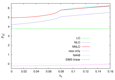
It has been already noticed, seeย [1] and Fig.ย 1, that ChPT, at present, underestimates the curvature fsโ€ฒโ€ฒsubscriptsuperscript๐‘“โ€ฒโ€ฒ๐‘ f^{\prime\prime}_{s}. On the other hand there are indications that dispersive analysis techniques might help solving this problem: Fig.ย 7 in [1] shows that the dispersive result of [13] has a larger curvature then the two-loop result. Therefore, we do not consider this discrepancy a major problem for ChPT.

Refer to caption
Figure 1: The absolute value of the Fssubscript๐น๐‘ F_{s} formfactor at sโ„“=cosโกฮธ=0subscript๐‘ โ„“๐œƒ0s_{\ell}=\cos{\theta}=0 as a function of sฯ€subscript๐‘ ๐œ‹s_{\pi} (in $\textrm{Gev}^{2}$ units) above and below threshold. The NNLO result nicely reproduces the linear fit quoted in [6], but not the large negative curvature in [5]. The line at the bottom is the contribution coming from the $C_{i}$, which has a positive curvature.

7 New fits of the NLO constants (preliminary results)

As remarked in [14], many NNLO calculations are now available in three-flavour ChPT. Besides, new lattice and dispersive results and further experimental data are at our disposal too. A study of the predictive power of NNLO ChPT is needed, and therefore also an update of the $L_{i}$ fit.
For this reason we are working on a new program to perform this fit with many more observables implemented. So far we have included masses and decay constants, $K_{\ell 4}$ formfactors, $\pi\pi$ and $\pi K$ scattering lengths and the scalar pion radius. For now we rely on the resonance estimates of the $C_{i}$ used inย [1], although our plan is to achieve more information on them.

fit 10 [1] fit 10 iso NA48/2 $F_{K}/F_{\pi}$ All
$10^{3}L_{1}^{r}$ $0.43$ $0.40\pm 0.12$ $0.98$ $0.97$ $0.99\pm 0.13$
$10^{3}L_{2}^{r}$ $0.73$ $0.76\pm 0.12$ $0.78$ $0.79$ $0.60\pm 0.22$
$10^{3}L_{3}^{r}$ $-2.35$ $-2.40\pm 0.37$ $-3.14$ $-3.12$ $-3.07\pm 0.59$
$10^{3}L_{4}^{r}$ $\equiv 0$ $\equiv 0$ $\equiv 0$ $\equiv 0$ $0.65\pm 0.64$
$10^{3}L_{5}^{r}$ $0.97$ $0.97\pm 0.11$ $0.93$ $0.72$ $0.53\pm 0.10$
$10^{3}L_{6}^{r}$ $\equiv 0$ $\equiv 0$ $\equiv 0$ $\equiv 0$ $0.07\pm 0.65$
$10^{3}L_{7}^{r}$ $-0.31$ $-0.30\pm 0.15$ $-0.30$ $-0.26$ $-0.21\pm 0.15$
$10^{3}L_{8}^{r}$ $0.59$ $0.61\pm 0.20$ $0.59$ $0.48$ $0.37\pm 0.17$
$\chi^{2}$ (dof) $0.25$ (1) $0.17$ (1) $0.19$ (1) $0.78$ (4)
Table 5: Preliminary results for the fits. $L_{9}\equiv 0.59\times 10^{-3}$ everywhere, as found from the vector pion radius in [15]. See text for a longer discussion

.

Our first preliminary results are summarized in Tab.ย 5. In the second column we quote fit 10 of [1]. This was found using the available linear fit for $K_{\ell 4}$ of [6], $F_{K}/F_{\pi}=1.22$, the kaon and eta masses with isospin breaking corrections included and setting $L_{4}\equiv L_{6}\equiv 0$. In the column labeled fit 10 iso we quote the fit we find using the same input as fit 10 but without including isospin breaking. As you see the two fits are in good agreement. The column NA48/2 relies on the new experimental data fromย [5]. We checked that the fit does not change including the curvature fsโ€ฒโ€ฒsubscriptsuperscript๐‘“โ€ฒโ€ฒ๐‘ f^{\prime\prime}_{s}. With this fit ChPT predicts the value fsโ€ฒโ€ฒ=โˆ’0.90subscriptsuperscript๐‘“โ€ฒโ€ฒ๐‘ 0.90f^{\prime\prime}_{s}=-0.90 to be compared with the experimental one fsโ€ฒโ€ฒ=โˆ’1.58ยฑ0.064subscriptsuperscript๐‘“โ€ฒโ€ฒ๐‘ plus-or-minus1.580.064f^{\prime\prime}_{s}=-1.58\pm 0.064. Note that the fit inย [5] shows large correlations between the slope and the curvature of the Fssubscript๐น๐‘ F_{s} formfactor which have not been taken into account yet. The values of $L_{1}$ and $L_{3}$ change drastically. The third column shows the fit obtained changing the ratio $F_{K}/F_{\pi}$ to $1.19$. This affects mainly $L_{5}$ and $L_{8}$. The last column shows the fit obtained letting $L_{4}$ and $L_{6}$ free, and adding $a^{0}_{0}$, $a^{2}_{0}$, $a^{1/2}_{0}$, $a^{3/2}_{0}$ and the scalar pion radius. The value obtained for $L_{4}$ is larger then expected. Some more comment can be found inย [16].

8 Conclusions

We have performed a systematic search for relations between observables that allow a test of ChPT at NNLO order in a $C_{i}$-independent way. We studied in detail the relations for the $\pi\pi$, $\pi K$ scattering and $K_{\ell 4}$ since for these cases enough experimental and/or dispersion theory results exist.

The resulting picture is that ChPT at NNLO mostly works but there are troublesome cases. The $\pi\pi$ system alone works well. The $\pi K$ system alone works satisfactorily but with some discrepancies. The same can be said for the combinations of both systems. A common part in these two cases is the presence of $a^{-}_{3}$ . Comparing $\pi K$ scattering and $K_{\ell 4}$ leads to a clear contradiction which needs further investigation.

Acknowledgments

IJ gratefully acknowledges an Early Stage Researcher position supported by the EU-RTN Programme, Contract No. MRTNโ€“CT-2006-035482, (FLAVIAnet). This work is supported in part by the European Commission RTN network, Contract MRTN-CT-2006-035482 (FLAVIAnet), European Community-Research Infrastructure Integrating Activity โ€œStudy of Strongly Interacting Matterโ€ (HadronPhysics2, Grant Agreement n. 227431) and the Swedish Research Council. We thank the organizers for a very pleasant meeting.

References

  • [1] G.ย Amorรณs, J.ย Bijnens and P.ย Talavera, Nucl. Phys. B 602 (2001) 87 [hep-ph/0101127].
  • [2] J.ย Bijnens and I.ย Jemos, 0906.3118 [hep-ph], to be published in Eur.ย Phys.ย J.ย  C .
  • [3] G.ย Colangelo, J.ย Gasser and H.ย Leutwyler, Nucl. Phys. B 603 (2001) 125 [hep-ph/0103088].
  • [4] P.ย Buettiker, S.ย Descotes-Genon and B.ย Moussallam, Eur.ย Phys.ย J.ย  C 33 (2004) 409 [hep-ph/0310283].
  • [5] J.ย R.ย Batley et al. [NA48/2 Collaboration], Eur.ย Phys.ย J.ย  C 54 (2008) 411.
  • [6] S.ย Pislak et al. [BNL-E865 Collaboration], Phys.ย Rev.ย Lett.ย  87 (2001) 221801 [hep-ex/0106071].
  • [7] J.ย Bijnens, P.ย Dhonte and P.ย Talavera, J. High Energy Phys. 0401 (2004) 050 [hep-ph/0401039].
  • [8] J.ย Bijnens, P.ย Dhonte and P.ย Talavera, J. High Energy Phys. 0405 (2004) 036 [hep-ph/0404150].
  • [9] G.ย Amorรณs, J.ย Bijnens and P.ย Talavera, Nucl. Phys. B 585 (2000) 293 [Erratum-ibid.ย  B 598 (2001) 665] [hep-ph/0003258].
  • [10] K.ย Kampf and B.ย Moussallam, C 47 (2006) 723 Eur.ย Phys.ย J.ย  C [hep-ph/0604125].
  • [11] J.ย Bijnens, G.ย Colangelo, G.ย Ecker and J.ย Gasser, hep-ph/9411311.
  • [12] G.ย Amorรณs and J.ย Bijnens, J.ย Phys.ย  G 25 (1999) 1607 [hep-ph/9902463].
  • [13] J.ย Bijnens, G.ย Colangelo and J.ย Gasser, Nucl. Phys. B B 427 (1994) 427 [hep-ph/9403390].
  • [14] J.ย Bijnens, Prog.ย Part.ย Nucl.ย Phys.ย  58 (2007) 521 [hep-ph/0604043].
  • [15] J.ย Bijnens and P.ย Talavera, J. High Energy Phys. 0203 (2002) 046 [hep-ph/0203049].
  • [16] J.ย Bijnens, talk at this conference.