$B^{+}$ and $D^{+}_{s}$ Decay Constants from Belle and Babar

Abstract

The Belle and Babar experiments have measured the branching fractions for $B^{+}\!\rightarrow\!\tau^{+}\nu$ and $D^{+}_{s}\!\rightarrow\!\mu^{+}\nu$ decays. From these measurements one can extract the $B^{+}$ and $D^{+}_{s}$ decay constants, which can be compared to lattice QCD calculations. For the $D^{+}_{s}$ decay constant, there is currently a $2.1\sigma$ difference between the calculated value and the measured value.

1 Introduction

Both the Belle belle and Babar babar experiments have measured the branching fractions for $B^{+}\!\rightarrow\!\tau^{+}\nu$ and $D^{+}_{s}\!\rightarrow\!\mu^{+}\nu$ decays charge-conjugates . These decays proceed via the annihilation diagram of Fig. 1. Within the Standard Model (SM), the predicted rates are

$${\cal B}(B^{+}\!\rightarrow\!\tau^{+}\nu) = \tau_{B^{+}}\,\frac{G^{2}_{F}}{8\pi}|V_{ub}|^{2}f^{2}_{B^{+}}\,m^{2}_{\tau}\,m_{B^{+}}\biggl{(}1-\frac{m^{2}_{\tau}}{m^{2}_{B^{+}}}\biggr{)}^{2}$$ (1)

$${\cal B}(D^{+}_{s}\!\rightarrow\!\ell^{+}\nu) = \tau_{D_{s}}\,\frac{G^{2}_{F}}{8\pi}|V_{cs}|^{2}f^{2}_{D_{s}}\,m^{2}_{\ell}\,m_{D_{s}}\biggl{(}1-\frac{m^{2}_{\ell}}{m^{2}_{D_{s}}}\biggr{)}^{2}\,.$$ (2)

For the $D^{+}_{s}$, all parameters on the right-hand-side except for $f_{D_{s}}$ are well-known. The Cabibbo-Kobayashi-Maskawa (CKM) matrix element $|V_{cs}|$ is well-constrained by a global fit to several experimental observables and unitarity of the CKM matrix. Thus a measurement of ${\cal B}(D^{+}_{s}\!\rightarrow\!\mu^{+}\nu)$ allows one to determine the decay constant $f_{D_{s}}$. This can be compared to QCD lattice calculations, which have become relatively precise. For the $B^{+}$, the CKM matrix element $|V_{ub}|$ is known to only 9%; this is nonetheless more precise than measurements of ${\cal B}(B^{+}\!\rightarrow\!\ell^{+}\nu)$ and allows one to extract $f_{B}$.

Figure 1: Annihilation diagram for a heavy meson decaying to a lepton and neutrino.

2 Measurement of $B^{+}\!\rightarrow\!\tau^{+}\nu$

Belle has done two $B^{+}\!\rightarrow\!\tau^{+}\nu$ analyses btaunu_belle_old ; btaunu_belle ; the most recent one used 605 fb^-1 of data and obtained evidence for a signal. This analysis employed a semileptonic tag: one $B$ in an event is fully reconstructed as $B^{-}\!\rightarrow\!D^{(*)0}\ell^{-}\bar{\nu}$, where $D^{*0}\!\rightarrow\!D^{0}\pi^{0}\!,\,D^{0}\gamma$ and $D^{0}\!\rightarrow\!K^{-}\pi^{+}(\pi^{0}),\,K^{-}\pi^{+}\pi^{-}\pi^{+}$. The signal decays $\tau^{+}\!\rightarrow\!\mu^{+}\nu_{\mu}\bar{\nu}_{\tau},\,e^{+}\nu_{e}\bar{\nu}_{\tau}$ and $\tau^{+}\!\rightarrow\!\pi^{+}\bar{\nu}_{\tau}$ are then searched for by reconstructing a single track not associated with the tag side. The signal yield is obtained by fitting the distribution of $E_{\rm ECL}$, which is the energy sum of calorimeter clusters not associated with a charged track. A peak near $E_{\rm ECL}\!=\!0$ indicates a $\tau^{+}\!\rightarrow\!\ell^{+}\nu_{\ell}\bar{\nu}_{\tau}$ or $\tau^{+}\!\rightarrow\!\pi^{+}\bar{\nu}_{\tau}$ decay. The main backgrounds are $b\!\rightarrow\!c$ processes and $e^{+}e^{-}\!\rightarrow\!q\bar{q}$ continuum events. The fit is unbinned and uses a likelihood function

$${\cal L} = \frac{e^{-\sum_{j}n_{j}}}{N!}\,\prod_{i}\sum_{j}n_{j}\,f_{j}(E_{i})\,,$$ (3)

where $i$ runs over all events ($N$), $j$ runs over all signal and background categories, $n_{j}$ is the yield of category $j$, and $f_{j}$ is the probability density function (PDF) for category $j$. The branching fraction is calculated as ${\cal B}=n_{s}/(2\cdot\varepsilon\cdot N_{B^{+}B^{-}})$, where $\varepsilon$ is the reconstruction efficiency as calculated from Monte Carlo (MC) simulation. The fit results are listed in Table 1, and the fit projections are shown in Fig. 2. The systematic errors are dominated by uncertainty in the background PDF and the tag reconstruction efficiency. The overall result is

$${\cal B}(B^{+}\!\rightarrow\!\tau^{+}\nu)\Bigr{|}_{\rm Belle} = \Bigl{(}1.65\,^{+0.38}_{-0.37}\,{}^{+0.35}_{-0.37}\Bigr{)}\times 10^{-4}\,,$$ (4)

where the first error is statistical and the second is systematic.

Decay Mode	Signal Yield	$\varepsilon$ (%)	${\cal B}\times 10^{4}$
$\tau^{-}\!\rightarrow\!e^{-}\bar{\nu}\nu_{\tau}$	$78\,^{+23}_{-22}$	0.059	$2.02\,^{+0.59}_{-0.56}$
$\tau^{-}\!\rightarrow\!\mu^{-}\bar{\nu}\nu_{\tau}$	$15\,^{+18}_{-17}$	0.037	$0.62\,^{+0.76}_{-0.71}$
$\tau^{-}\!\rightarrow\!\pi^{-}\nu_{\tau}$	$58\,^{+21}_{-20}$	0.047	$1.88\,^{+0.70}_{-0.66}$
Combined	$154\,^{+36}_{-35}$	0.143	$1.65\,^{+0.38}_{-0.37}$

Table 1: Fit results for $B^{+}\!\rightarrow\!\tau^{+}\nu$, from Belle btaunu_belle . The data sample corresponds to 605 fb^-1.

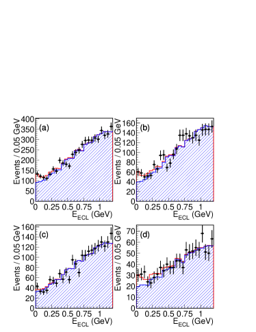
Figure 2: $E_{ECL}$ distribution of data events (points) and fit projections for $B^{+}\!\rightarrow\!\tau^{+}\nu$, from Belle btaunu_belle . (a) all $\tau$ decay modes combined; (b) $\tau^{-}\!\rightarrow\!e^{-}\bar{\nu}_{e}\,\nu_{\tau}$; (c) $\tau^{-}\!\rightarrow\!\mu^{-}\bar{\nu}_{\mu}\,\nu_{\tau}$; (d) $\tau^{-}\!\rightarrow\!\pi^{-}\nu_{\tau}$. The open and hatched histograms correspond to signal and background, respectively.

Babar has published two analyses of $B^{+}\!\rightarrow\!\tau^{+}\nu$ decays: one using a semileptonic tag btaunu_babar_semi and the other using a hadronic tag btaunu_babar_hadr . Both analyses use data samples consisting of $383\times 10^{6}$ $B\overline{B}$ pairs. The former is similar to that used in the Belle analysis: the tag side is reconstructed as $B^{-}\!\rightarrow\!D^{(*)0}\ell^{-}\bar{\nu}_{\ell}$, where $D^{*0}\!\rightarrow\!D^{0}\pi^{0},\,D^{0}\gamma$ and $D^{0}\!\rightarrow\!K^{-}\pi^{+}(\pi^{0}),\,K^{-}\pi^{+}\pi^{-}\pi^{+}\!,\,K_{S}\,\pi^{+}\pi^{-}$. Babar searches for $\tau^{+}\!\rightarrow\!\ell^{+}\nu_{\ell}\bar{\nu}_{\tau}$, $\tau^{+}\!\rightarrow\!\pi^{+}\bar{\nu}_{\tau}$, and also $\tau^{+}\!\rightarrow\!\pi^{+}\pi^{0}\bar{\nu}_{\tau}$, where for the last mode the $\pi^{+}\pi^{0}$ mass is required to be near that of the $\rho^{+}$. The signal is identified by plotting $E_{\rm extra}$, the energy sum of calorimeter clusters not associated with a charged track; a peak near zero indicates $\tau^{+}$ decay. The signal yield is obtained by counting events in a signal region, e.g., $E_{\rm extra}<0.50$, and subtracting off background as estimated from $E_{\rm extra}$ sidebands. The number of events in the final sample is 245, the background estimate is $222\pm 13$, and the resulting branching fraction is $(0.9\,\pm 0.6{\rm\ (stat.)}\,\pm 0.1{\rm\ (syst.)})\times 10^{-4}$.

The Babar hadronic-tag analysis is more complicated. The tagging side is reconstructed as $B^{-}\!\rightarrow\!D^{(*)0}X^{-}$, where $X^{-}$ denotes a hadronic system of total charge $-1$ composed of $n_{1}(\pi^{\pm})$, $n_{2}(K^{\pm})$, $n_{3}(K^{0}_{S})$, and $n_{4}(\pi^{0})$, where $n_{1}+n_{2}\leq 5$, $n_{3}\leq 2$, and $n_{4}\leq 2$. The $D^{(*)0}$ is reconstructed in the same channels as those used for the semileptonic analysis, as is the $\tau^{+}$ on the signal side. A background subtraction is done on the tag side. The signal yield is obtained by counting events in an $E_{\rm extra}$ signal region and subtracting off background as estimated from an $E_{\rm extra}$ sideband. There are 24 signal candidates and $14.3\pm 3.0$ estimated background events; the resulting branching fraction is $(1.8\,^{+0.9}_{-0.8}\,\pm 0.4\,\pm 0.2)\times 10^{-4}$, where the first error is statistical, the second is due to the background uncertainty, and the third is due to other systematic sources. The data is shown in Fig. 3 along with projections of the fit. This result is consistent with the semileptonic-tagged result; combining the two gives

$${\cal B}(B^{+}\!\rightarrow\!\tau^{+}\nu)\Bigr{|}_{\rm Babar} = \Bigl{(}1.2\,\pm 0.4{\rm\ (stat.)}\,\pm 0.3{\rm\ (bkg.)}\,\pm 0.2{\rm\ (syst.)}\Bigr{)}\times 10^{-4}\,.$$ (5)

This is consistent with the Belle result, Eq. (4).

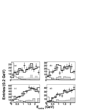
Figure 3: $E_{\rm extra}$ distribution of data events (points) and fit projections for $B^{+}\!\rightarrow\!\tau^{+}\nu$, from Babar using a hadronic tag btaunu_babar_hadr . (a) $\tau^{-}\!\rightarrow\!e^{-}\bar{\nu}_{e}\,\nu_{\tau}$; (b) $\tau^{-}\!\rightarrow\!\mu^{-}\bar{\nu}_{\mu}\,\nu_{\tau}$; (c) $\tau^{-}\!\rightarrow\!\pi^{-}\nu_{\tau}$; (d) $\tau^{-}\!\rightarrow\!\pi^{-}\pi^{0}\nu_{\tau}$. The hatched histogram shows the combinatorial background component, and, for comparison, the open histogram shows $B^{+}\!\rightarrow\!\tau^{+}\nu$ signal for a branching fraction of 0.3%.

3 Measurement of $D^{+}_{s}\!\rightarrow\!\mu^{+}\nu$

The Belle analysis of $D^{+}_{s}\!\rightarrow\!\mu^{+}\nu$ decays dsmunu_belle uses 548 fb^-1 of data and searches for $e^{+}e^{-}\!\rightarrow\!DKD^{*}_{s}\,n(\pi,\gamma)$, where the primary $D$ and $K$ can be charged or neutral; the $D^{*}_{s}$ is “reconstructed” (see below) via $D^{+}_{s}\gamma$; $n(\pi,\gamma)\equiv X$ signifies any number of additional pions and up to one photon (from fragmentation); the $D$ is reconstructed via $D\!\rightarrow\!K\,n(\pi)$, where $n\!=\!1,2,3$; and neutral kaons are reconstructed via $K^{0}_{S}\!\rightarrow\!\pi^{+}\pi^{-}$. If the primary $K$ is charged, both it and the $D$ must have flavors opposite to that of the $D^{+}_{s}$; these constitute a “right-sign” (RS) sample. If the flavors are not both opposite, the event is categorized as “wrong-sign” (WS) and used to parameterize the background. The same classification applies to primary neutral $K$ events, except for these only the $D$ flavor must be opposite to that of the $D^{+}_{s}$ for the event to be classified as RS.

The decay sequence is identified via a recoil mass technique. First, the recoil mass of the $D$, $K$, and $X$ particles is calculated and required to be within 150 MeV/$c^{2}$ of $M_{D^{*}_{s}}$; then the $\gamma$ is included and the recoil mass is required to be within 150 MeV/$c^{2}$ of $M_{D^{+}_{s}}$; and finally, the $\mu^{+}$ is included and the recoil mass required to be within 0.55 GeV/$c^{2}$ of zero. The final $DK\,X\gamma\mu^{+}$ recoil mass distribution is shown in Fig. 4; a sharp peak is observed near zero, indicating $D^{+}_{s}\!\rightarrow\!\mu^{+}\nu$ decay.

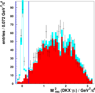
Figure 4: Recoil mass distribution for $e^{+}e^{-}\!\rightarrow\!DK\,X\gamma\mu^{+}$, from Belle dsmunu_belle .

The analysis is complicated by the fact that the recoil mass technique is very sensitive to the number of tracks in an event and the track reconstruction efficiency, as all tracks must be reconstructed for the recoil mass to be accurate. As it is difficult to simulate track multiplicity accurately due to uncertainties in quark fragmentation, the data is divided into bins of $n^{R}_{x}$, the number of “primary particles” reconstructed in an event. Here, a primary particle is one that is not a daughter of any particle reconstructed in the event. The minimum value for $n^{R}_{x}$ is three, corresponding to $e^{+}e^{-}\!\rightarrow\!DKD^{*}_{s}$ without any additional particles from fragmentation. The data is then fit in two dimensions, $DK\,X\gamma$ recoil mass vs. $n^{R}_{x}$ (see Fig. 5). The signal PDF is obtained from MC and modeled separately for different values of $n^{T}_{x}$, the true number of primary particles in an event ($n^{T}_{x}$ can differ from $n^{R}_{x}$ due to particles being lost or incorrectly assigned).

The branching fraction is obtained from two fits: the first fit uses the $DK\,X\gamma$ recoil mass spectrum and yields the number of $D^{+}_{s}$ candidates; the result is $N_{D_{s}}=32100\,\pm 870{\rm\ (stat)}\,\pm 1210{\rm\ (syst)}$. For this fit the background shape is taken from the WS sample and the background levels floated in the fit. The second fit uses the $DK\,X\gamma\mu^{+}$ recoil mass spectrum and yields the number of $D^{+}_{s}\!\rightarrow\!\mu^{+}\nu$ candidates; the result is $N_{\mu\nu}=169\,\pm 16{\rm\ (stat)}\,\pm 8{\rm\ (syst)}$. For this fit the background shape is taken from a RS “$D^{+}_{s}\!\rightarrow\!e^{+}\nu$” sample, i.e., all selection criteria are the same except that an electron candidate is required instead of a muon candidate. As true $D^{+}_{s}\!\rightarrow\!e^{+}\nu$ decays are suppressed by $\sim\!10^{-5}$, this sample provides a good model of the $D^{+}_{s}\!\rightarrow\!\mu^{+}\nu$ background. The systematic errors listed are dominated by uncertainties in the signal and background PDFs and are obtained by varying the shapes of these PDFs. The branching fraction is the ratio $N_{\mu\nu}/N_{D_{s}}$, corrected for the ratio of reconstruction efficiencies. The result is

$${\cal B}(D^{+}_{s}\!\rightarrow\!\mu^{+}\nu)\Bigl{|}_{\rm Belle} = \Bigl{(}6.44\,\pm 0.76{\rm\ (stat.)}\,\pm 0.57{\rm\ (syst.)}\Bigr{)}\times 10^{-3}\,.$$ (6)

Figure 5: Two-dimensional $DK\,X\gamma$ recoil mass vs. $n^{R}_{x}$ distribution (see text), from Belle dsmunu_belle .

The Babar experiment searches for $D^{+}_{s}\!\rightarrow\!\mu^{+}\nu$ dsmunu_babar using 230 fb^-1 of data by fully reconstructing a flavor-specific $D^{(*)-},\,\overline{D}{}^{0}$, or $D^{-}_{s}$ decay on the tagging side. Tag candidates are reconstructed in the following modes: $\overline{D}{}^{0}\!\rightarrow\!K^{+}\pi^{-}(\pi^{0}),\,K^{+}\pi^{-}\pi^{+}\pi^{-}$; $D^{-}\!\rightarrow\!K^{+}\pi^{-}\pi^{-}(\pi^{0}),\,K^{0}_{S}\,\pi^{-}(\pi^{0}),\,K^{0}_{S}\,\pi^{-}\pi^{-}\pi^{+},\,\,K^{+}K^{-}\pi^{-},\,K^{0}_{S}\,K^{-}$; $D^{-}_{s}\!\rightarrow\!K^{0}_{S}K^{-},\,\phi\rho^{-}$; and $D^{*-}\!\rightarrow\!\overline{D}{}^{0}\pi^{-}$ with $\overline{D}{}^{0}\!\rightarrow\!K^{0}_{S}\,\pi^{+}\pi^{-}(\pi^{0}),\,K^{0}_{S}\,K^{+}K^{-},\,K^{0}_{S}\,\pi^{0}$. An isolated $\mu^{+}$ track is required. The neutrino momentum is taken to be the missing momentum in the event: $\vec{p}_{\nu}\equiv\vec{p}_{e^{+}e^{-}}\!-\vec{p}_{\rm rest}$. A photon is required and paired with the $D^{+}_{s}$ candidate to make a $D^{*+}_{s}$, and the mass difference $\Delta M\equiv M(\mu^{+}\nu\gamma)-M(\mu^{+}\nu)$ is calculated.

The data is subsequently divided into four subsamples: a tag-side mass sideband and a tag-side signal region for $\mu^{+}$ and $e^{+}$ candidates. For both lepton samples, the tag-side-sideband $\Delta M$ spectrum is subtracted from the tag-side-signal $\Delta M$ spectrum (Fig. 6), and then the sideband-subtracted $e^{+}$ spectrum is subtracted from the sideband-subtracted $\mu^{+}$ spectrum. The final $\Delta M$ distribution (Fig. 7a) is fit with signal and background PDFs; the signal yield obtained is $N_{\mu^{+}\nu}=489\,\pm 55$ events.

To determine the branching fraction, the signal yield is normalized to $D^{+}_{s}\!\rightarrow\!\phi\pi^{+}$ decays. Like the signal mode, the $D^{+}_{s}$ candidate is required to originate from $D^{*+}_{s}\!\rightarrow\!D^{+}_{s}\gamma$. The tag-side-sideband $\Delta M$ spectrum is subtracted from the tag-side-signal $\Delta M$ spectrum, and the resulting spectrum is fit with signal and background PDFs (Fig. 7b). The signal yield obtained is $N_{\phi\pi^{+}}=2093\,\pm 99$ events. Dividing $N_{\mu^{+}\nu}$ by $N_{\phi\pi^{+}}$ and correcting for the ratio of reconstruction efficiencies gives

$$\frac{\Gamma(D^{+}_{s}\!\rightarrow\!\mu^{+}\nu)}{\Gamma(D^{+}_{s}\!\rightarrow\!\phi\pi^{+})}\Bigl{|}_{\rm Babar} = 0.143\,\pm 0.018{\rm\ (stat.)}\,\pm 0.006{\rm\ (syst.)}\,.$$ (7)

For this analysis, the $\phi$ is reconstructed via $\phi\!\rightarrow\!K^{+}K^{-}$ with $|M_{K^{+}K^{-}}-M_{\phi}|\equiv\Delta M_{KK}<5.5$ MeV joncoleman . Conveniently, CLEO has measured the branching fraction ${\cal B}(D^{+}_{s}\!\rightarrow\!K^{+}K^{-}\pi^{+})$ for $\Delta M_{KK}=5{\rm\ MeV}$; the result is $(1.69\,\pm 0.08\,\pm 0.06)\%$ cleo_dskkp . To multiply the two results together to obtain ${\cal B}(D^{+}_{s}\!\rightarrow\!\mu^{+}\nu)$ requires dividing Eq. (7) by ${\cal B}(\phi\!\rightarrow\!K^{+}K^{-})=0.491$ and subtracting (in quadrature) the 1.2% uncertainty in ${\cal B}(\phi\!\rightarrow\!K^{+}K^{-})$ from the systematic error. In addition, Babar has subtracted off a small amount of $D^{+}_{s}\!\rightarrow\!f_{0}(980)(K^{+}K^{-})\pi^{+}$ background (48 events); as this process is included in the CLEO measurement, these events must be added back in to Babar’s $\phi\pi^{+}$ yield. Thus the Babar result becomes

$$\frac{\Gamma(D^{+}_{s}\!\rightarrow\!\mu^{+}\nu)}{\Gamma(D^{+}_{s}\!\rightarrow\!K^{+}K^{-}\pi^{+})}\biggr{|}_{\Delta M_{KK}=5.5{\rm\ MeV}} = 0.285\,\pm 0.035{\rm\ (stat.)}\,\pm 0.011{\rm\ (syst.)}\,.$$ (8)

Multiplying this by CLEO’s measurement gives

$${\cal B}(D^{+}_{s}\!\rightarrow\!\mu^{+}\nu)\Bigl{|}_{\rm Babar} = \Bigl{(}4.81\,\pm 0.63{\rm\ (stat.)}\,\pm 0.25{\rm\ (syst.)}\Bigr{)}\times 10^{-3}\,.$$ (9)

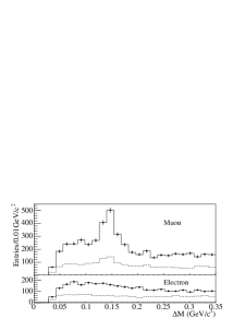
Figure 6: $\Delta M$ spectra for the tag-side sideband region (dashed) and tag-side signal region (solid) for $\mu^{+}$ (top) and $e^{+}$ (bottom) samples, from Babar dsmunu_babar .

 

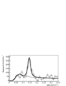
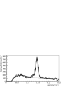
Figure 7: Background-subtracted $\Delta M$ spectra (see text) and projections of the fit result, from Babar dsmunu_babar . The left-most (right-most) distribution corresponds to $D^{+}_{s}\!\rightarrow\!\mu^{+}\nu$ ($D^{+}_{s}\!\rightarrow\!\phi\pi^{+}$) candidates. The dashed line is the background component, and the solid line is the signal plus background components combined.

4 Extraction of Decay Constants

The Belle and Babar collaborations have used their measurements of ${\cal B}(B^{+}\!\rightarrow\!\tau^{+}\nu)$ and Eq. (1) to calculate the product of the $B$ decay constant $f_{B}$ and the CKM matrix element $|V_{ub}|$. The results are

$$f_{B}\times|V_{ub}|\times 10^{4} = \left\{\begin{array}[]{l}9.7\,\pm 1.1{\rm\ (stat.)}\,^{+1.0}_{-1.1}{\rm\ (syst.)}{\rm\ GeV\ \ (Belle)}\\ \\ 7.2\,^{+2.0}_{-2.8}{\rm\ (stat.)}\,\pm 0.2{\rm\ (syst.)}{\rm\ GeV\ \ (Babar\ semileptonic)}\\ \\ 10.1\,^{+2.3}_{-2.5}{\rm\ (stat.)}\,^{+1.2}_{-1.5}{\rm\ (syst.)}{\rm\ GeV\ \ (Babar\ hadronic)}.\end{array}\right.$$

Taking a weighted average gives

$$f_{B}\times|V_{ub}|\,_{\rm(Belle+Babar\ avg.)} = (9.2\pm 1.2)\times 10^{-4}{\rm\ \ GeV}\,,$$ (11)

and dividing by the Particle Data Group value $|V_{ub}|=(0.393\,\pm 0.036)\%$ pdg_vub gives

$$f_{B}\bigr{|}_{\rm(Belle+Babar\ avg.)} = 233\pm 37~{}{\rm MeV}\,.$$ (12)

This value is $1\sigma$ higher than the most recent lattice QCD results, that of the HPQCD collaboration ($190\,\pm 13$ MeV hpqcd_b ) and that of the Fermilab/MILC collaboration ($195\,\pm 11$ MeV milc ).

The Heavy Flavor Averaging Group (HFAG) has calculated a world average (WA) value for ${\cal B}(D^{+}_{s}\!\rightarrow\!\mu^{+}\nu)$ and used this to determine a WA value for the $D^{+}_{s}$ decay constant $f_{D_{s}}$ hfag_ds . This value can be compared to recent lattice QCD calculations; a significant difference could indicate new physics. The WA value for $f_{D_{s}}$ is obtained by inverting Eq. (2):

$$f_{D_{s}} = \frac{1}{G_{F}|V_{cs}|m_{\ell}\biggl{(}1-\frac{\displaystyle m^{2}_{\ell}}{\displaystyle m^{2}_{D_{s}}}\biggr{)}}\sqrt{\frac{8\pi\,{\cal B}(D^{+}_{s}\!\rightarrow\!\ell^{+}\nu)}{m_{D_{s}}\tau_{D_{s}}}}\,,$$ (13)

where, for ${\cal B}(D^{+}_{s}\!\rightarrow\!\ell^{+}\nu)$, the WA value is inserted. The error on $f_{D_{s}}$ is calculated as follows: values for variables on the right-hand-side of Eq. (13) are sampled from Gaussian distributions having means equal to the central values and standard deviations equal to their respective errors. The resulting values of $f_{D_{s}}$ are plotted, and the distribution is fit to a bifurcated Gaussian to obtain the $\pm 1\sigma$ errors.

The results of this procedure are shown in Fig. 8. Also included are measurements of ${\cal B}(D^{+}_{s}\!\rightarrow\!\mu^{+}\nu)$ cleo_dsmunu and ${\cal B}(D^{+}_{s}\!\rightarrow\!\tau^{+}\nu)$ cleo_dstaunu from CLEO. Thus there are three types of measurements: $f_{D_{s}}$ from the absolute $D^{+}_{s}\!\rightarrow\!\mu^{+}\nu$ branching fraction, $f_{D_{s}}$ from the absolute $D^{+}_{s}\!\rightarrow\!\tau^{+}\nu$ branching fraction, and $f_{D_{s}}$ from the $\Gamma(D^{+}_{s}\!\rightarrow\!\mu^{+}\nu)/\Gamma(D^{+}_{s}\!\rightarrow\!K^{+}K^{-}\pi^{+})$ ratio. The overall WA value is obtained by averaging the three results, carefully accounting for correlations such as the input values for $|V_{cs}|$ and $\tau_{D_{s}}$. The result is $256.9\,\pm 6.8$ MeV. This value is higher than the two most precise lattice QCD results, that of the HPQCD ($241\,\pm 3$ MeV hpqcd_ds ) and Fermilab/MILC ($249\,\pm 11$ MeV milc ) collaborations. The weighted average of the theory results is $241.5\,\pm 2.9$ MeV, which differs from the HFAG result by $2.1\sigma$.

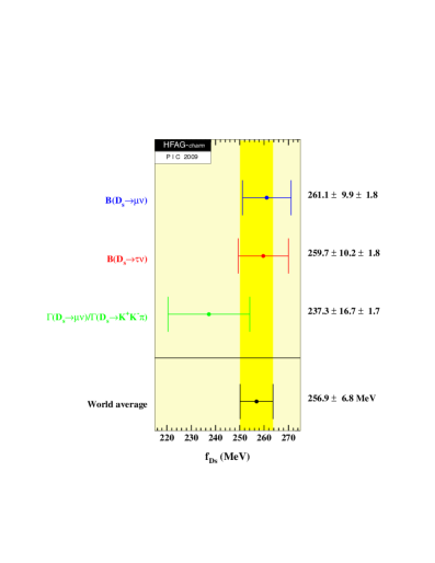
Figure 8: Heavy Flavor Averaging Group (HFAG) WA value for $f_{D_{s}}$, from Ref. hfag_ds . For each measurement, the first error listed is the total uncorrelated error, and the second error is the total correlated error (mostly from $\tau_{D_{s}}$).

5 Summary

In summary, Belle has observed $B^{+}\!\rightarrow\!\tau^{+}\nu$ with $3.8\sigma$ significance. From the measured branching fraction they determine the product $f_{B}\times|V_{ub}|$. Babar has observed $B^{+}\!\rightarrow\!\tau^{+}\nu$ with $2.6\sigma$ significance and has also measured the branching fraction to determine $f_{B}\times|V_{ub}|$. The results from the two experiments are consistent; the weighted average has 13% precision and is consistent with lattice QCD calculations.

For $D^{+}_{s}\!\rightarrow\!\mu^{+}\nu$ decays, Belle has observed this mode using a recoil mass technique and has measured the branching fraction with 15% precision. Babar has also observed this mode and has measured the branching fraction relative to that for $D^{+}_{s}\!\rightarrow\!\phi\pi^{+}$ with 13% precision. Dividing this by the branching fraction for $\phi\!\rightarrow\!K^{+}K^{-}$ and including $D^{+}_{s}\!\rightarrow\!f_{0}(980)(K^{+}K^{-})\pi^{+}$ decays allows one to multiply by CLEO’s measurement of ${\cal B}(D^{+}_{s}\!\rightarrow\!K^{+}K^{-}\pi^{+})$ to obtain ${\cal B}(D^{+}_{s}\!\rightarrow\!\mu^{+}\nu)$. The Heavy Flavor Averaging Group has used the Belle and Babar measurements and also measurements from CLEO to calculate a world average value for $f_{D_{s}}$; the result is $256.9\,\pm 6.8$ MeV. This value is $2.1\sigma$ higher than the average of two recent lattice QCD calculations; the difference could indicate new physics.

References

- (1) Belle experiment, http://belle.kek.jp/.
- (2) Babar experiment, http://www.slac.stanford.edu/BFROOT/.
- (3) Unless noted otherwise, charge-conjugate modes are implicitly included.
- (4) K. Ikado et al. (Belle Collab.), Phys. Rev. Lett. 97, 251802 (1996).
- (5) I. Adachi et al. (Belle Collab.), arXiv:0809.3834.
- (6) B. Aubert et al. (Babar Collab.), Phys. Rev. D 76, 052002 (2007). A preliminary (unpublished) result with 20% more data is presented in B. Aubert et al. (Babar Collab.), arXiv:0809.4027.
- (7) B. Aubert et al. (Babar Collab.), Phys. Rev. D 77, 011107 (2008).
- (8) R. Widhalm et al. (Belle Collab.), Phys. Rev. Lett. 100, 241801 (2008).
- (9) B. Aubert et al. (Babar Collab.), Phys. Rev. Lett. 98, 141801 (2007).
- (10) J. Coleman (Babar), private communication.
- (11) J. P. Alexander et al. (CLEO Collab.), Phys. Rev. Lett. 100, 161804 (2008).
- (12) C. Amsler et al. (Particle Data Group), Phys. Lett. B 667, 1 (2008) and 2009 partial update for the 2010 edition (http://pdg.lbl.gov).
- (13) E. Gámiz et al. (HPQCD Collab.), Phys. Rev. D 80 014503 (2009).
- (14) C. Bernard et al. (Fermilab/MILC Collab.), arXiv:0904.1895.
-
(15)
Heavy Flavor Averaging Group (HFAG),
http://www.slac.stanford.edu/xorg/hfag/charm/index.html. - (16) J. P. Alexander et al. (CLEO Collab.), Phys. Rev. D 79 052001 (2009).
- (17) J. P. Alexander et al. (CLEO Collab.), Phys. Rev. D 79 052001 (2009). P. Onyisi et al. (CLEO Collab.), Phys. Rev. D 79 052002 (2009).
- (18) E. Follana et al. (HPQCD Collab.), Phys. Rev. Lett. 100, 062002 (2008).