Separating inner and outer contributions in gravitational lenses using the perturbative method.

Abstract

Context. This paper presents a reconstruction of the gravitational lens SL2S02176-0513 using the singular perturbative method presented in Alard 2007, MNRAS Letters, 382, 58 and Alard, C., 2008, MNRAS, 388, 375.

Aims. The ability of the perturbative method to separate the inner and outer contributions of the potential in gravitational lenses is tested using SL2S02176-0513. In this lens, the gravitational field of the central galaxy is dominated by a nearby group of galaxies located at a distance of a few critical radius.

Methods. The perturbative functionals are re-constructed using local polynomials. The polynomial interpolation is smoothed using Fourier series, and numerically fitted to HST data using a non-linear minimization procedure. The potential inside and outside the critical circle is derived from the reconstruction of the perturbative fields.

Results. The inner and outer potential contours are very different. The inner contours are consistent with the central galaxy, while the outer contours are fully consistent with the perturbation introduced by the group of galaxies.

Conclusions. The ability of the perturbative method to separate the inner and outer contribution is confirmed, and indicates that in the perturbative approach the field of the central deflector can be separated from outer perturbations. The separation of the inner and outer contribution is especially important for the study of the shape of dark matter halo’s as well as for the statistical analysis of the effect of dark matter substructures.

1 Introduction.

Gravitational lenses are a precious astrophysical tools to probe the mass distribution of dark halo’s. The recent results obtained by Clowe etal (2006) are a good example of the ability of gravitational lensing to probe complex mass distributions. In this context the recently perturbative approach (Alard 2007), and its application to the reconstruction of strong gravitational lenses (Alard 2008, 2009), is of particular interest since this approach relates directly the properties of the images to the lens potential. The lens SL2S02176-0513 is the second lens to be reconstructed using the perturbative approach. The first re-construction of a gravitational lens using the perturbative approach is described in Alard (2009), this work offer a general presentation of the methods and algorithms that will be used in this paper. The lens SL2S02176-0513 was already modeled by Tu etal (2009) using conventional methods. Tu etal (2009) identified 3 components in the lens: the stellar component, the dark matter halo associated with the galaxy, and finally an external influence coming from a nearby group of galaxies. The surface density of the bright part is modeled as a Sersic profile, while the dark component is represented with an elliptical pseudo isothermal sphere. The center of the dark component is supposed to be the same as the center of light. The external component is represented with a singular isothermal sphere (SIS). The position of the SIS is not a free parameter, it is derived from X ray observations (Geach etal 2007). The model proposed by Tu etal (2009) is physically motivated, although it has a large number of free parameters and the exploration of the parameter space is always a difficult task. The minimization surface in the parameter space is complex, with the usual presence of several minima’s of similar depth resulting in a degeneracy of the solution. Thus the problem in itself is not to find a possible solution but to explore the range of solutions consistent with the data. The family of solutions have common properties and these common properties are the really interesting quantities. The perturbative approach has the advantage to describe the lens using a general singular perturbative expansion. A given perturbative expansion corresponds to a family of models, and not to a single model. An important asset in this approach is that the general properties of the solution are directly related to the physical properties of the images. This direct relation indicates that the perturbative reconstruction is not degenerated. A general description of the perturbative methods and of its application to the inversion of gravitational lenses is available in Alard (2009).

2 The perturbative approach in gravitational lensing.

This section will present a brief summary of the singular perturbative approach in gravitational lensing, for more details, see Alard (2007). The perturbation is singular since the un-perturbed solution is a circle with an infinite number of points, while the perturbed solution has only a finite number of points. It is important to note that this perturbative approach is not related to conventional regular perturbative method already explored in gravitational lensing. For an example of regular perturbative theory in gravitational lensing, see for instance Vegetti & Koopmans (2009). The un-perturbed situation is represented by a circular lens with potential $\phi_{0}(r)$, and a point source with null impact parameter. In the perturbed situation the source has an impact parameter ${\bf r_{S}}$, and the lens is perturbed by the non-circular potential $\psi(r,\theta)$. Both perturbations, ${\bf r_{S}}$ and $\psi$ are assumed to be of the same order $\epsilon$:

$$\begin{cases}{\bf r_{S}}&=\epsilon\ {\bf r_{s}}\\ \phi&=\phi_{0}+\epsilon\ \psi\end{cases}$$ (1)

Similar ideas were explored by Blandford & Kovner (1998), the main difference with Alard (2007) is the derivation of analytical equations describing image formation. These equations relate directly the properties of the images to the local potential; the derivation of these equations will be presented now. Note that for convenience the unit of the coordinate system is the critical radius. Thus by definition in this coordinate system the critical radius is situated at $r=1$. As a consequence, in the continuation of this work all distances and their associated quantities (errors,..,) will be expressed in unit of the critical radius. In response to this perturbation the radial position of the image will be shifted by an amount $dr$ with respect to the un-perturbed point on the critical circle. The new radial position of the image is:

$$r=1+\epsilon\ dr$$ (2)

The response $dr$ to the perturbation can be evaluated by solving the lens equation in the perturbative regime, leading to the perturbative lens equation:

$${\bf r_{s}}=\left(\kappa_{2}\ dr-f_{1}\right)\ {\bf u_{r}}-\frac{df_{0}}{d\theta}\ {\bf u_{\theta}}$$ (3)

and $\kappa_{2}=1-\left[\frac{d^{2}\phi_{0}}{dr^{2}}\right]_{(r=1)}$

This equation corresponds to Eq. (8) in Alard (2007). Considering that the source has a mean impact parameter ${\bf r_{0}}$, the position in the source plane may be re-written: ${\bf r_{S}=\tilde{r_{S}}+r_{0}}$. Assuming Cartesian coordinates $(x_{0},y_{0})$ for the vector ${\bf r_{0}}$ Eq.  3 reads:

$${\bf\tilde{r}_{s}}=\left(\kappa_{2}\ dr-\tilde{f}_{1}\right)\ {\bf u_{r}}-\frac{d\tilde{f}_{0}}{d\theta}\ {\bf u_{\theta}}$$ (4)

For a circular source with radius $R_{0}$, the perturbative response $dr$ takes the simple following form (Alard 2007, Eq. 12):

$$dr=\frac{1}{\kappa_{2}}\left[\tilde{f}_{1}\pm\sqrt{R_{0}^{2}-\left(\frac{d\tilde{f}_{0}}{d\theta}\right)^{2}}\right]$$ (5)

To conclude it is important to note that Eq. ( 3) depends on $\kappa_{2}$. However this variable can be eliminated from Eq. ( 3) by re-normalizing the fields: $f_{n}=\frac{f_{n}}{\kappa_{2}}$, and the source plane coordinates, ${\bf r_{s}}=\frac{{\bf r_{s}}}{\kappa_{2}}$ (mass sheet degeneracy). These re-normalized variables will be adopted in the continuation of this work. The re-normalization is equivalent to solving Eq.’s ( 3) and ( 5) for $\kappa_{2}=1$. The variable $\kappa_{2}$ will re-appear when the re-normalized quantities are converted to the original quantities.

3 Pre-processing of the HST data.

The gravitational lens SL2S02176-0513 (Cabanac etal. 2007, SL2S public domain) was observed by HST in 3 spectral domain, F475W, F606W, F814W, with an exposure time of 400 sec. Cosmics cleaning and image re-interpolation to a common grid are performed using software’s from the ISIS package (Alard 2000). Considering that in the radial direction the arc size is only of a few pixels, to facilitate the numerical calculations (convolution with the PSf for instance) it is useful to work on a finer grid. The images were re-mapped to a grid with a pixel size smaller by a factor of 2, which is small enough to avoid aliasing problems. But note that this re-sampling is only a numerical convenience, and that the computing of statistical estimates is performed using the orginal data, and not the re-sampled and interpolated (correlated) data. Note also that at this level, no astrometric registration is performed, and that the system of coordinate is the system of the initial HST image. However the final result will presented in a proper astrometric system (North up, and East left). Note also that there is a large number of cosmics in these images, and the local density of cosmics is sometime very high. When too many nearby cosmics are detected within a small area, the area is flagged, and will be considered cautiously, or even rejected. Finally, the 3 cleaned and re-centered images are stacked, and the background is subtracted to produce a reference image of the arc system. Two color illustrations of the arc system are also provided in Fig.’s ( 1)).

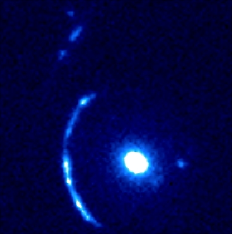
Figure 1: Color image for SL2S02176-0513 reconstructed from 3 noise filtered HST images in 3 bands.

4 Lens inversion.

The lens SL2S02176-0513 forms a system of image resembling a near cusp configuration, with a large arc on the left side of the deflector and a small counter image on the other side (see Fig.  1). The 4 bright parts in the images have similar brightness and are probably the image of a unique area in the source (see Fig.  2). Tu etal (2009) have associated another fainter bright detail with these features (see Fig.  2). But we will see that this association is unlikely since this detail has a slightly different color and additionally would require a complicated field shape to be associated with the other 4 bright features.

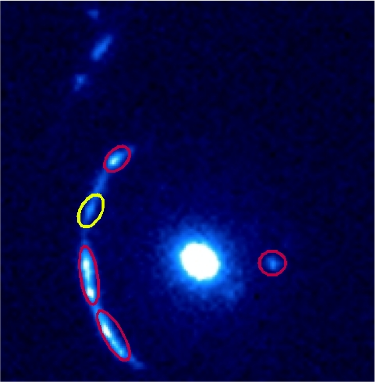
Figure 2: The red contours indicates the 4 bright areas visible in the image of the source formed by the lens. The flux in these areas is similar which suggests that these area corresponds to the same part of the source plane. The yellow contour indicates a detail associated with the 4 other bright details by Tu etal (2009). Note that this detail is fainter and most importantly has a slightly different color which makes this association unlikely.

4.1 Estimation of the critical circle.

The critical circle is estimated by fitting a circle to the mean position of the images. The center and radius of the circle are adjusted. The non-linear adjustment procedure starts from a circle centered on the small galaxy at the center of the image. The initial estimate for the circle radius is the mean distance of the images to the center. A non linear optimization shows that the best center is close to the initial guess and that the optimal radius is close to 30.5 pixels, with a pixel size of $0.049^{\prime\prime}$ the critical circle radius $R_{C}$ is: $1.49^{\prime\prime}$. Note that the final result will not depend upon the particular choice of a given critical circle. Taking another circle close to this one would change a little the estimation of the perturbative fields, but the total background plus perturbation would remain the same.

4.2 General properties of the solution.

An approximate solution will be derived from the properties of the circular source solution. To estimate the circular source solution, the outer contour of the bright area in the source will be approximated with a circle. Note that since the bright areas of the image are composed of 2 nearby bright spots, the corresponding source region is also composed of 2 bright features. In the circular approximation, we will consider the circular envelope of these 2 bright spots. It would have been possible to consider the bright spots one by one, but the determination of the local parameters would have been less accurate. This approximation of the source may not be very accurate, the typical error on the field estimation will be on the order of the source outer contour deviations from circularity. However this approximation is sufficient to derive the general properties of the solution, and in particular the behavior of the $\frac{df_{0}}{d\theta}$ field near the minimum. For circular sources the perturbative fields are directly related to the data (see Sec. 3, and Eq. ( 5). The field $f_{1}$ corresponds to the mean radial position of the image, while the reconstruction of the field $\frac{df_{0}}{d\theta}$ is more complicated and will be explained in details in this section. Note that the direct relation between the perturbative fields and the data is possible only in bright areas, and that as a consequence $\frac{df_{0}}{d\theta}$ and $f_{1}$ will have to be interpolated in dark areas. The derivation of the general properties of $\frac{d\tilde{f}_{0}}{d\theta}$ require some specific guess of the local behavior of this field in the region of image formation. Images form in minimum of $|\frac{d\tilde{f}_{0}}{d\theta}|$, the local behavior of $\frac{df_{0}}{d\theta}$ near the minimum is of 2 types: linear behavior for small images , for large images (caustics) $\frac{df_{0}}{d\theta}$ behaves like an higher order polynomial (see Alard 2009 for more details). All images of the source bright region are small (see Fig  2), as a consequence a local linear model will be adopted. The parameters of the local linear model are estimated using Eq. ( 5). Given the values of the 4 local slopes and the constraint that no image are formed in dark areas ($\frac{df_{0}}{d\theta}>$ source radius), the general shape of the field is reconstructed (see Fig  3). Note that the sign of the slope for two consecutive images has to be different to avoid a crossing of the zero line between the images and the formation of an additional image. Note also that at this level the sign of $\frac{df_{0}}{d\theta}$ is degenerate. Implicitly, since only one feature is seen in the upper right bight area, the current model assumes that the 2 bight spots visible in the other images are merged here. This is the simplest model consistent with the data. Another possibility is to assume that the 2 images are not merged and that the yellow contour in Fig. ( 2) corresponds to the image of the second bright spot, as considered by Tu etal. (2009). However since the separation between the images is large the slope of the local model would have to be small. To be consistent with this small local slope and the presence of a dark area between the 2 images, a higher order Fourier expansion of $\frac{df_{0}}{d\theta}$ would be required (see Fig.  4). Additionally the color diagrams of the 4 bright spots (red contours in Fig.  2) are very similar, but the color diagram of the fifth bright spot (yellow contour in Fig.  2) is significantly different (see Fig.  5). This slight but significant difference in color shows that the fifth bright spot is not associated with the same source area as the 4 other bight spots. This is a confirmation that the solution proposed in Tu et al (2009) is not consistent with the data, and that that the simplest perturbative model (Fig.  3) predicts the correct association of the images.

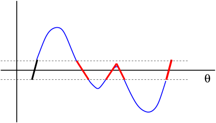
Figure 3:

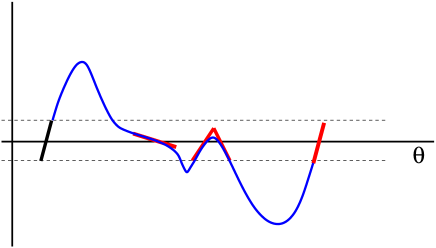
Figure 4:

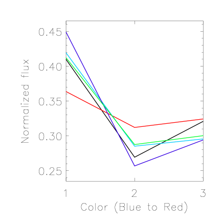
Figure 5: The raw HST flux in each photometric bands normalized by the total flux in the 3 bands. The red diagram represents the color of the fifth bright area (yellow contour in Fig.  2), the other diagrams represent the color of the 4 other bright areas (red contours in Fig.  2). The color diagram of the fifth bright area is different at the $4\sigma$ levels from the mean diagram of the 4 other bright areas.

5 Fitting of the perturbative fields.

A qualitative evaluation of the perturbative fields has been performed in Sec.  4.2, we will turn now to a quantitative evaluation of $\frac{df_{0}}{d\theta}$. The quantitative evaluation will be conducted in two steps, first an approximate guess will be evaluated using the circular source solution, and second this guess will be refined by fitting the data.

5.1 First numerical guess.

As explained in Section  4.2 the field $f_{1}$ in the circular source approximation is directly related to the mean image radial position. To reconstruct this field a Fourier series of order 3 is fitted to the mean image position. Fitting a higher order Fourier series does not improve significantly the fit, and a lower order expansion is not a good match to the data. Let’s now turn to the estimation of $\frac{df_{0}}{d\theta}$. The solution presented in the former section (see Fig.  2) is evaluated using the following piecewise numerical model: first order polynomials in each area where an image of the source is present, second order polynomials in dark areas. Eq  5 shows that the image angular size is given by the condition $\frac{df_{0}}{d\theta}=R_{0}$. Thus, for a linear model, $k\frac{1}{2}\Delta\theta=R_{0}$, with $\Delta\theta$ the angular size of the image, and $k$ the slope of the linear model. The coefficients of the second order polynomials in the dark areas are evaluated using continuity conditions, the constraint that no images should be formed in dark areas ($\frac{df_{0}}{d\theta}>R_{0}$), and the constraint that the solution should be as smooth as possible. The piecewise polynomial solution is fitted with an order 3 Fourier series. The Fourier expansion will be used as a first guess for the final fitting of the perturbative fields. The numerical guess are presented in Fig  6. More details about the reconstruction of the numerical guess are availbale in Alard (2009), Sec. 4.3 and 4.4.

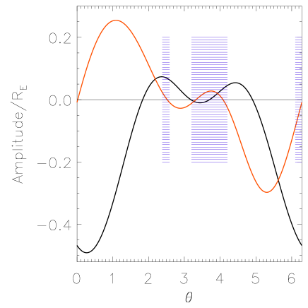
Figure 6:

5.2 Final fitting of the fields.

The final fitting of the fields is conducted by reconstructing the images of the source and comparing these images with the HST data by chi-square estimation. The reconstruction of the images for a given set of perturbative fields will be performed using the Warren & Dye (2003) method. The source is represented with a linear combination of basis functions. The basis functions are identical to the functionals used for image subtraction (Alard  Lupton 1998, Alard 2000). The images of each basis function is reconstructed and convolved with the HST PSF. The HST PSF is estimated using the Tiny Tim software (Krist 1995). Finally, the convolved images of the basis function are fitted to the HST data using a linear least-square method. The quality of the fit is evaluated by chi-square estimation. This fitting of the data for a given set of perturbative fields is conducted iteratively. The inital estimation starts from the numerical guess presented in the former section, leading to an initial chi-square estimation. This initial guess is improved iteratively using Nelder & Mead (1965) simplex method until convergence is reached. The final result is presented in Fig  7.

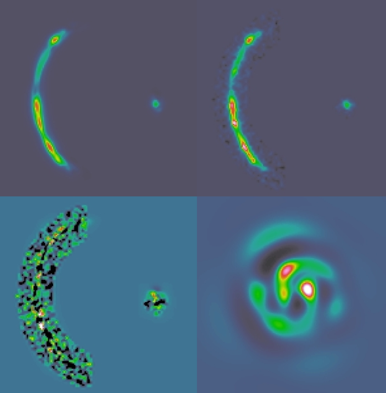
Figure 7:

5.3 Noise.

5.3.1 Chi-square of the fit.

The model and the data are compared in a small region around the arcs with total number of pixels $N$. The Poisson weighted difference $R_{i}$ between the model at pixel $i$, $M_{i}$ and the HST data $D_{i}$ is very close to a Gaussian (see Fig.  8). Considering that the model has $N_{P}$ parameters, the 13 parameters of the perturbative expansion , and the 57 source model parameters, the chi-square is, $\chi_{2/dof}=\frac{1}{N-N_{P}}\sum_{i}R_{i}^{2}\simeq 1.33$. Changing a little the size of the area, either reducing it by moving closer to the center of the arcs, or enlarging the area does not significantly change the chi-square value.

5.3.2 Errors on the reconstruction of the perturbative fields.

Alard (2009) investigated the errors on the reconstruction of the perturbative fields and found that the errors due to the Poissonian noise were negligible. The re-construction noise is dominated by the errors introduced by the first order approximation of the lens equation (see Alard 2009, Sec. 4.6). The results for SL2S02176-0513 are very similar, the mean error on the Fourier coefficients of the perturbative expansion due to the Poisson noise is: $\sigma_{P}=\simeq 0.25\ 10^{-3}$ (in unit of the critical radius). The error due to the first order approximation $\sigma_{A}$ is evaluated by comparing the position of the bright details in the HST image and the model reconstruction. The measurement procedure is described in Alard (2009) Sec 4.5.2. The numerical estimation of the error on the position between model and data is : $\simeq 0.6\%R_{C}$. This positional error is identical to the error on the perturbative fields (see Alard 2009, Sec 4.6.2). Assuming that the errors on the Fourier coefficient are similar the error is $\sigma_{A}\simeq 2.5e-03$ which is much larger that the error due to the Poisson noise $\sigma_{P}$. As a consequence the Poissonian noise will be neglected. Following Alard (2009) Sec 4.6.3, the error on the reconstruction of the potential iso-contours, $\delta\phi_{iso}$ is:

$$\delta\phi_{iso}=\sigma_{P}\sqrt{\sum_{j=1}^{3}\frac{1}{j^{2}}}\simeq 0.0026$$

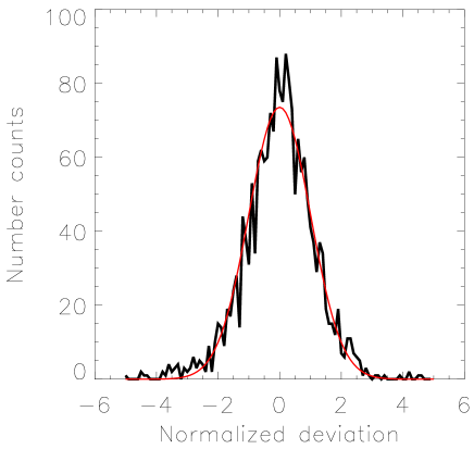
Figure 8:

6 Properties of the lens.

The perturbative expansion is related directly to the properties of the lens potential. In particular Eq. (C.1) in Alard (2009) relates $f_{0}$ to the potential iso-contours.

6.1 Potential iso-contours.

The solution of the perturbative lens equation (Eq  5) depends on $\tilde{f}_{i}=f_{i}+x_{0}cos\theta+y_{0}sin\theta$, $i=0,1$, and $x_{0}$, $y_{0}$, the source impact parameters. The potential iso-contour is related to $f_{0}$ by the following equation: : $dr=-f_{0}$ (see Alard (2009), Eq C.1). Since only $\tilde{f}_{0}$ is known, and since the impact parameters are unknown the first order Fourier terms of $f_{0}$ are unknown. The first order Fourier terms corresponds to the centering of the potential and do not affect the shape of the potential iso-contours (see Alard 2009, Sec 6) .As a consequence the shape of the potential iso-contours will be computed using the Fourier expansion of $\tilde{f}_{0}$ from order 2 to the maximum order (order 3). However, the inner potential iso-contour do not depend on the impact parameters, as a consequence the relevant first order terms are meaningfull. But the corresponding terms are very small, indicating that the center of the inner potential iso-contour is very close to the centre of light. An important asset of the singular perturbative approach is that the inner and outer contribution to the potential can be separated. The potential generated by the lens projected density inside the critical circle corresponds to the coefficients $a_{n}$ and $b_{n}$ in the expansion of the potential (see Eq’s B.1 and B.2 in Alard 2009). The potential generated by the the projected density outside the critical circle corresponds to $c_{n}$ and $d_{n}$. Eq B.3 in Alard (2009) relates the Fourier expansion of the perturbative fields to $a_{n}$, $b_{n}$, $c_{n}$ and $d_{n}$. As a consequence it is possible to reconstruct the potential corresponding to the projected density within and outside the critical circle. The potential near the critical circle is dominated by the outer contribution (see Fig  9). Furthermore, the shape of the inner and outer are not the same. Both the ellipticity and orientation of the inner and outer contribution are very different. Using the second order Fourier terms it is straightforward to estimate the elliptical parameters for the inner and outer potential. The elliptical contour equation in a coordinate system aligned with the ellipse axis reads:

$$(1-\eta)x^{2}+(1+\eta)y^{2}=R_{0}^{2}$$

To first order in $\eta$:

$$r=R_{0}\left(1+\frac{\eta}{2}\cos 2\theta\right)$$

Considering that $r=1+dr$, in a general coordinate system where the mis-alignment between the ellipse main axis and the abscissa axis is $\psi$:

$$dr=\frac{\eta}{2}\cos\left(2(\theta-\psi)\right)$$ (6)

An identification with the potential iso-contour equation $dr=-f_{0}$ leads to, inner contribution: $\eta_{i}=0.028\pm 0.005$ and $\psi_{i}=-31.7^{\circ}\pm 5^{\circ}$, outer contribution: $\eta_{o}=0.121\pm 0.005$ and $\psi_{o}=9.79^{\circ}\pm 1^{\circ}$. Note that at first order in $\eta$, the ellipticity is equal to $\eta$. It is important to remind that as a consequence of the mass-sheet degeneracy the scaling factor $\kappa_{2}$ is unknown (see Eq’s  4 and  5). In practice, experiments with dark matter halo’s extracted form numerical simulations shows that $\kappa_{2}\simeq 1$ (Peirani etal 2008). Note that $\kappa_{2}$ is local quantity and that $\kappa_{2}\simeq 1$ does not require that the background potential is fully isothermal. In the continuation of this paper it will be assumed that $\kappa_{2}=1$, but that in practice $\kappa_{2}$ may be slightly different from unity, which would imply a re-scaling of the perturbative functionals. However this re-scaling would affect the ellipticity, but not other properties like the ellipse inclination angle.

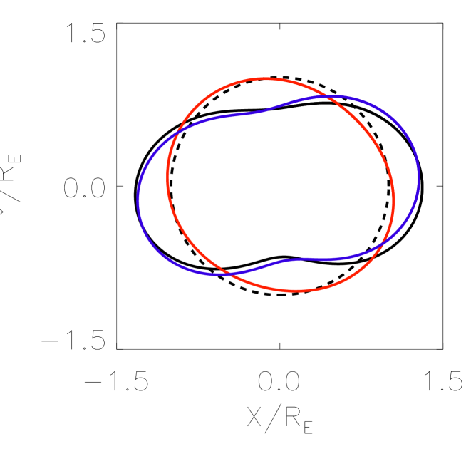
Figure 9: The potential iso-contours, the black curve corresponds to the potential generated by the whole mass distribution, the blue curve corresponds to the potential generated by the outer projected mass distribution and the red curve corresponds the potential generated by the projected mass distribution inside the critical circle. Note that the first order Fourier terms have not been included in the expansion (due to a degeneracy with the impact parameters). As a consequence the position of the contour center is unknown for the outer distribution. In this plot the direction of the vertical axis is parallel to the North (North is up and East is left). To improve the readibility of the plot, the amplitude of the non-circular distrosion have been exagerated (by a factor of 5).

6.2 Comparison to observational properties of the lens.

It is interesting to compare the inner potential iso-contour with the iso-contours of the galaxy situated at the center of the lens. To estimate the photometric properties of the lens a Sersic profile was fitted to the light distribution. A similar procedure was already performed by Tu etal (2009). The surface mass density profile is identical to Tu etal (2009), Eq. 1, except that the quantity $\frac{b_{n}}{R_{e}^{1/n}}$ is obviously degenerate and was replaced with a single parameter. The iso-contour of this elliptical profile depends on $\eta$ (the ellipticity) and on the inclination angle of the ellipse main axis $\phi$. The fitting of the Sersic profile is conducted by minimizing the Poisson weighted residual between the Sersic model and a compilation of the 3 HST images. Note that the Sersic model is convolved with the HST PSF, and that the non-linear minimization is performed using Nelder and Mead (1965) simplex method. The results of this fitting procedure is: $\eta=0.207\pm 0.014$ and $\psi=-33.2^{\circ}\pm 2.4^{\circ}$. Tu etal (2009) found: $\eta=0.14\pm 0.06$ and $\psi=12\pm 6^{\circ}$. The error bar were evaluated using Monte-Carlo simulation (Poisson noise was added to the images). The ellipticity $\eta=0.207$ is compatible with Tu etal (2009), but the consistency of the ellipse inclination is quite poor. The distance between the two measurements is larger than 3 $\sigma$. Tu etal (2009) suggests that the errors may be dominated by systematic effects. To investigate this issue the fit was performed separately on the 3 HST images. The results are the following (from blue to red photometric band): ($-35.1^{\circ}$, $-44.9^{\circ}$, $-25.1^{\circ})$, with average $35^{\circ}$, and scatter $9.9^{\circ}$. Note that estimating the scatter with such a small number of measurements is not very accurate. Considering the averaged value of the 3 measurements, no particular systematic is detected in this analysis. The reason for the different inclination angle found by Tu etal (2009) is unclear. Considering the photometric properties found in the present work, the comparison with the iso-contours of the inner potential reads: difference in inclination, $1.5^{\circ}\pm 5.5^{\circ}$, ellipticities, $0.207\pm 0.014$ (galaxy) and $0.028\pm 0.005$. Obviously the inclination angle are compatible, which suggests that the dark matter halo surrounding the galaxy has a similar orientation. The comparison of the ellipticities is model dependent. Assuming the following toy model: a dominant isothermal dark halo with ellipticity $\eta_{d}$, to first order in $\eta$ the ellipticity of the potential iso-contour is: $3\eta_{d}$. Thus if the ellipticity of the dark halo is the same as the ellipticity of the light distribution, the potential iso-contour ellipticity would be: $\eta=0.069\pm 0.005$. The difference in ellipticity between the inner potential iso-contour is: $0.04\pm 0.007$. Thus the ellipticities are not consistent, and this simple model suggests that ellipticity of the dark halo is probably smaller smaller that the ellipticity of the light distribution. Let’s turn now to the contribution of the outer projected distribution to the potential. Tu etal (2009) pointed out that the central galaxy is close to a group of galaxies observed by Geach etal (2007). The great difference between the outer and inner contribution is due to the influence of this group on the outer component. A simple model is to consider two isothermal components for the central galaxy dark matter halo and for the mass of the group. Let assume that these 2 isothermal components have respectively a velocity dispersion $\sigma_{0}$ and $\sigma_{1}$, the potential for an isothermal system reads: $\phi=c_{0}\sigma^{2}r$, where $c_{0}$ is a constant. The central galaxy is very close to the center of the coordinate system, thus

$$\phi_{0}=c_{0}\sigma_{0}^{2}r$$

in a coordinate system where the center of the group is on the abscissa axis at a distance $r_{1}ll1$, the potential of the group reads:

$$\phi_{1}=c_{0}\sigma_{1}^{2}|\bf r-\bf r_{1}|$$

The critical condition implies that $\left[\frac{\partial\phi_{0}}{\partial r}\right]_{r=1}=1$, thus $c_{0}=\frac{1}{\sigma_{0}^{2}}$, and as a consequence:

$$\phi_{1}=\frac{\sigma_{1}^{2}}{\sigma_{0}^{2}}|\bf r-\bf r_{1}|$$

To estimate the contribution of the group to the field $f_{0}$, we will evaluate $f_{0}=\phi_{1}(r,\theta)$ at $r=1$. To second order in $\frac{r}{r_{1}}$:

$$\phi_{1}(r,\theta)=\frac{\sigma_{1}^{2}}{\sigma_{0}^{2}}\left(r_{1}+\frac{r^{2}}{4r_{1}}-r\cos\theta-\frac{r^{2}}{4r_{1}}\right)$$

the coefficient of the second order Fourier term of $f_{0}$ at $r=1$ is: $-\frac{\sigma_{1}^{2}}{4\sigma_{0}^{2}r_{1}}$. An identification with the iso-contour equation (Eq.  6), shows that:

$$\frac{\sigma_{1}}{\sigma_{0}}=\sqrt{2\eta r_{1}}$$

In the former section it was estimated that $\eta=0.121$, and adopting the position of the center of the group proposed by Tu etal (2009), $r_{1}\simeq 36$ (in units of the critical radius). As consequence, $\frac{\sigma_{1}}{\sigma_{0}}=\simeq 2.95$. Geach etal estimate that $\sigma_{1}=520\pm 120km/s$ from the $\sigma-T_{X}$ relation and $\sigma_{1}=770\pm 170km/s$ from the X ray temperature. Tu etal. (2009) estimate from photometric data that $\sigma_{0}=218^{+43}_{-28}$. Assuming that the mass is dominated by the dark halo, respectively: $\frac{\sigma_{1}}{\sigma_{0}}=2.38\pm 0.72$, and $\frac{\sigma_{1}}{\sigma_{0}}=3.53\pm 1.04$. Both value are compatible with $\frac{\sigma_{1}}{\sigma_{0}}\simeq 2.95$ inferred from the outer contribution to the potential estimated using the perturbative approach. Let’s now estimate the compatibility between the inclination angles. The group center is situated in a direction at $\theta_{G}=16^{\circ}$ from the abscissa axis. Since the uncertainty on the group center position is 10 arc-sec (Tu etal 2009) this translate in an error on $\theta_{G}$ of $10.3^{\circ}$. This angle should match the inclination angle of the elliptical contour of the outer potential which is: $9.79^{\circ}\pm 1^{\circ}$. Considering the errors, these 2 angles are consistent.

7 Discussion

The re-construction of the lens SL2S02176-0513 using the perturbative method indicates that the gravitational field in this lens is dominated by an outer contribution due to a nearby group of galaxies. The separation of the inner and outer potential contribution using the perturbative method is free of any assumptions. Furthermore, the perturbative analysis shows that the inner potential contribution is small but statistically significant. The orientation of the inner potential iso-contour is consistent with the shape of the central galaxy luminosity contours, which illustrates the accuracy of the perturbative re-construction. The outer potential iso-contours reconstructed using the perturbative method are consistent with the perturbation introduced by the group of galaxies. Both the ellipticity and orientation match the group properties. The analysis of this gravitational lens demonstrates the ability of the perturbative approach to separate the inner and outer contribution to the potential without making any particular assumptions. This lens is very special since the outer contribution to the potential is well identified and dominates other contribution to the outer potential. In general for other lenses the identification of the perturbators situated outside the critical radius is not obvious and using conventional methods the ability to re-construct the proper lens potential is compromised. Since the perturbative approach does not contain such flaws, and that the inner and outer contribution to the potential can be separated it is clear that an un-biased re-construction of the lens properties can be performed. This capability of the perturbative method to re-construct the inner properties of the lens are especially useful to interpret complex gravitational lenses (see Alard 2009). Such an analysis will be also very useful in the statistical analysis of the perturbation introduced by sub-structures in dark matter halo’s (see Alard 2008, and Peirani etal 2008).

- (1) Alard, C., Lupton, R., 1998, ApJ, 503, 325
- (2) Alard, C., 2000, A&AS, 144, 363
- (3) Alard, C., 2007, MNRAS Letters, 382, 58
- (4) Alard, C., 2008, MNRAS, 388, 375
- (5) Alard, C., 2009, A&A, in press
- (6) Blandford, R.D., Kovner, I., 1988, Phys. Rev. A 38, 4028
- (7) Clowe, D., Bradac, M., Gonzalez, A., Markevitch, M., Randall, S., Jones, C., Zaritsky, D., 2006, ApJ, 648 Letters, 109
- (8) Geach, J., Simpson, C., Rawlings, S., Read, A. M., Watson, M., 2007, MNRAS, 381, 1369
- (9) Krist, J., 1995, ASPC, 77, 349
- (10) Nelder, J., Mead, R., 1965, Computer Journal, 7, 308
- (11) Tu, H. and 9 co-hautors, 2009, A&A, 501, 475
- (12) Vegetti, S., Koopmans, L., 2009, MNRAS, 392, 945