Flow-Based Propagators for the SEQUENCE
and Related Global Constraints

Abstract

We propose new filtering algorithms for the Sequence constraint and some extensions of the Sequence constraint based on network flows. We enforce domain consistency on the Sequence constraint in $O(n^{2})$ time down a branch of the search tree. This improves upon the best existing domain consistency algorithm by a factor of $O(\log n)$. The flows used in these algorithms are derived from a linear program. Some of them differ from the flows used to propagate global constraints like Gcc since the domains of the variables are encoded as costs on the edges rather than capacities. Such flows are efficient for maintaining bounds consistency over large domains and may be useful for other global constraints.

1 Introduction

Graph based algorithms play a very important role in constraint programming, especially within propagators for global constraints. For example, Regin’s propagator for the AllDifferent constraint is based on a perfect matching algorithm [1], whilst his propagator for the Gcc constraint is based on a network flow algorithm [2]. Both these graph algorithms are derived from the bipartite value graph, in which nodes represent variables and values, and edges represent domains. For example, the Gcc propagator finds a flow in such a graph in which each unit of flow represents the assignment of a particular value to a variable. In this paper, we identify a new way to build graph based propagators for global constraints: we convert the global constraint into a linear program and then convert this into a network flow. These encodings contain several novelties. For example, variables domain bounds can be encoded as costs along the edges. We apply this approach to the Sequence family of constraints. Our results widen the class of global constraints which can be propagated using flow-based algorithms. We conjecture that these methods will be useful to propagate other global constraints.

2 Background

A constraint satisfaction problem (CSP) consists of a set of variables, each with a finite domain of values, and a set of constraints specifying allowed combinations of values for subsets of variables. We use capital letters for variables (e.g. $X$, $Y$ and $S$), and lower case for values (e.g. $d$ and $d_{i}$). A solution is an assignment of values to the variables satisfying the constraints. Constraint solvers typically explore partial assignments enforcing a local consistency property using either specialized or general purpose propagation algorithms. A support for a constraint $C$ is a tuple that assigns a value to each variable from its domain which satisfies $C$. A bounds support is a tuple that assigns a value to each variable which is between the maximum and minimum in its domain which satisfies $C$. A constraint is domain consistent (DC) iff for each variable $X_{i}$, every value in the domain of $X_{i}$ belongs to a support. A constraint is bounds consistent (BC) iff for each variable $X_{i}$, there is a bounds support for the maximum and minimum value in its domain. A CSP is DC/BC iff each constraint is DC/BC. A constraint is monotone iff there exists a total ordering $\prec$ of the domain values such that for any two values $v$, $w$ if $v\prec w$ then $v$ is substitutable for $w$ in any support for $C$.

We also give some background on flows. A flow network is a weighted directed graph $G=(V,E)$ where each edge $e$ has a capacity between non-negative integers $l(e)$ and $u(e)$, and an integer cost $w(e)$. A feasible flow in a flow network between a source $(s)$ and a sink $(t)$, $(s,t)$-flow, is a function $f:E\rightarrow\mathbb{Z}^{+}$ that satisfies two conditions: $f(e)\in[l(e),u(e)]$, $\forall e\in E$ and the flow conservation law that ensures that the amount of incoming flow should be equal to the amount of outgoing flow for all nodes except the source and the sink. The value of a $(s,t)$-flow is the amount of flow leaving the sink $s$. The cost of a flow $f$ is $w(f)=\sum_{e\in E}w(e)f(e)$. A minimum cost flow is a feasible flow with the minimum cost. The Ford-Fulkerson algorithm can find a feasible flow in $O(\phi(f)|E|)$ time. If $w(e)\in\mathbb{Z}$, $\forall e\in E$, then a minimum cost feasible flow can be found using the successive shortest path algorithm in $O(\phi(f)SPP)$ time, where $SPP$ is the complexity of finding a shortest path in the residual graph. Given a $(s,t)$-flow $f$ in $G(V,E)$, the residual graph $G_{f}$ is the directed graph $(V,E_{f})$, where $E_{f}$ is

$$\{e\ \mbox{with cost}\ w(e)\ \mbox{and capacity}\ 0..(u(e)-f(e))~{}|~{}e=(u,v)\in E,f(e)<u(e)\}\bigcup$$

$$\{e\ \mbox{with cost}\ -w(e)\ \mbox{and capacity}\ 0..(f(e)-l(e))~{}|~{}e=(u,v)\in E,l(e)<f(e)\}$$

There are other asymptotically faster but more complex algorithms for finding either feasible or minimum-cost flows [3].

In our flow-based encodings, a consistency check will correspond to finding a feasible or minimum cost flow. To enforce DC, we therefore need an algorithm that, given a minimum cost flow of cost $w(f)$ and an edge $e$ checks if an extra unit flow can be pushed (or removed) through the edge $e$ and the cost of the resulting flow is less than or equal to a given threshold $T$. We use the residual graph to construct such an algorithm. Suppose we need to check if an extra unit flow can be pushed through an edge $e=(u,v)$. Let $e^{\prime}=(u,v)$ be the corresponding arc in the residual graph. If $w(e)=0$, $\forall e\in E$, then it is sufficient to compute strongly connected components (SCC) in the residual graph. An extra unit flow can be pushed through an edge $e$ iff both ends of the edge $e^{\prime}$ are in the same strongly connected component. If $w(e)\in\mathbb{Z}$, $\forall e\in E$, the shortest path $p$ between $v$ and $u$ in the residual graph has to be computed. The minimal cost of pushing an extra unit flow through an edge $e$ equals $w(f)+w(p)+w(e)$. If $w(f)+w(p)+w(e)>T$, then we cannot push an extra unit through $e$. Similarly, we can check if we can remove a unit flow through an edge.

3 The Sequence Constraint

The Sequence constraint was introduced by Beldiceanu and Contejean [4]. It constrains the number of values taken from a given set in any sequence of $k$ variables. It is useful in staff rostering to specify, for example, that every employee has at least 2 days off in any 7 day period. Another application is sequencing cars along a production line (prob001 in CSPLib). It can specify, for example, that at most 1 in 3 cars along the production line has a sun-roof. The Sequence constraint can be defined in terms of a conjunction of Among constraints. $\mbox{\sc Among}(l,u,[X_{1},\ldots,X_{k}],v)$ holds iff $l\leq|\{i|X_{i}\in v\}|\leq u$. That is, between $l$ and $u$ of the $k$ variables take values in $v$. The Among constraint can be encoded by channelling into 0/1 variables using $Y_{i}\leftrightarrow(X_{i}\in v)$ and $l\leq\sum_{i=1}^{k}Y_{i}\leq u$. Since the constraint graph of this encoding is Berge-acyclic, this does not hinder propagation. Consequently, we will simplify notation and consider Among (and Sequence) on 0/1 variables and $v=\{1\}$. If $l=0$, Among is an AtMost constraint. AtMost is monotone since, given a support, we also have support for any larger assignment [5]. The Sequence constraint is a conjunction of overlapping Among constraints. More precisely, $\mbox{\sc Sequence}(l,u,k,[X_{1},\ldots,X_{n}],v)$ holds iff for $1\leq i\leq n-k+1$, $\mbox{\sc Among}(l,u,[X_{i},\ldots,X_{i+k-1}],v)$ holds. A sequence like $X_{i},\ldots,X_{i+k-1}$ is a window. It is easy to see that this decomposition hinders propagation. If $l=0$, Sequence is an AtMostSeq constraint. Decomposition in this case does not hinder propagation. Enforcing DC on the decomposition of an AtMostSeq constraint is equivalent to enforcing DC on the AtMostSeq constraint  [5].

Several filtering algorithms exist for Sequence and related constraints. Regin and Puget proposed a filtering algorithm for the Global Sequencing constraint (Gsc) that combines a Sequence and a global cardinality constraint (Gcc) [6]. Beldiceanu and Carlsson suggested a greedy filtering algorithm for the CardPath constraint that can be used to propagate the Sequence constraint, but this may hinder propagation [7]. Regin decomposed Gsc into a set of variable disjoint Among and Gcc constraints [8]. Again, this hinders propagation. Bessiere et al. [5] encoded Sequence using a Slide constraint, and give a domain consistency propagator that runs in $O(nd^{k-1})$ time. van Hoeve et al. [9] proposed two filtering algorithms that establish domain consistency. The first is based on an encoding into a Regular constraint and runs in $O(n2^{k})$ time, whilst the second is based on cumulative sums and runs in $O(n^{3})$ time down a branch of the search tree. Finally, Brand et al. [10] studied a number of different encodings of the Sequence constraint. Their asymptotically fastest encoding is based on separation theory and enforces domain consistency in $O(n^{2}\log n)$ time down the whole branch of a search tree. One of our contributions is to improve on this bound.

4 Flow-based Propagator for the Sequence Constraint

We will convert the Sequence constraint to a flow by means of a linear program (LP). We shall use $\mbox{\sc Sequence}(l,u,3,[X_{1},\ldots,X_{6}],v)$ as a running example. We can formulate this constraint simply and directly as an integer linear program:

$$l\leq X_{1}+X_{2}+X_{3} \leq u,$$

$$l\leq X_{2}+X_{3}+X_{4} \leq u,$$

$$l\leq X_{3}+X_{4}+X_{5} \leq u,$$

$$l\leq X_{4}+X_{5}+X_{6} \leq u$$

where $X_{i}\in\{0,1\}$. By introducing surplus/slack variables, $Y_{i}$ and $Z_{i}$, we convert this to a set of equalities:

$$X_{1}+X_{2}+X_{3}-Y_{1}=l, X_{1}+X_{2}+X_{3}+Z_{1}=u,$$

$$X_{2}+X_{3}+X_{4}-Y_{2}=l, X_{2}+X_{3}+X_{4}+Z_{2}=u,$$

$$X_{3}+X_{4}+X_{5}-Y_{3}=l, X_{3}+X_{4}+X_{5}+Z_{3}=u,$$

$$X_{4}+X_{5}+X_{6}-Y_{4}=l, X_{4}+X_{5}+X_{6}+Z_{4}=u$$

where $Y_{i},Z_{i}\geq 0$. In matrix form, this is:

$$\left(\setcounter{MaxMatrixCols}{14}\begin{smallmatrix}1&1&1&0&0&0&-1&0&0&0&0&0&0&0\\ 1&1&1&0&0&0&0&1&0&0&0&0&0&0\\ 0&1&1&1&0&0&0&0&-1&0&0&0&0&0\\ 0&1&1&1&0&0&0&0&0&1&0&0&0&0\\ 0&0&1&1&1&0&0&0&0&0&-1&0&0&0\\ 0&0&1&1&1&0&0&0&0&0&0&1&0&0\\ 0&0&0&1&1&1&0&0&0&0&0&0&-1&0\\ 0&0&0&1&1&1&0&0&0&0&0&0&0&1\end{smallmatrix}\right)\left(\begin{smallmatrix}X_{1}\\ \vdots\\ X_{6}\\ Y_{1}\\ Z_{1}\\ \vdots\\ Y_{4}\\ Z_{4}\end{smallmatrix}\right)=\left(\begin{smallmatrix}l\\ u\\ l\\ u\\ l\\ u\\ l\\ u\end{smallmatrix}\right)$$

This matrix has the consecutive ones property for columns: each column has a block of consecutive 1’s or $-1$’s and the remaining elements are 0’s. Consequently, we can apply the method of Veinott and Wagner [11] (also described in Application 9.6 of  [3]) to simplify the problem. We create a zero last row and subtract the $i$th row from $i+1$th row for $i=1$ to $2n$. These operations do not change the set of solutions. This gives:

$$\left(\setcounter{MaxMatrixCols}{14}\begin{smallmatrix}1&1&1&0&0&0&-1&0&0&0&0&0&0&0\\ 0&0&0&0&0&0&1&1&0&0&0&0&0&0\\ -1&0&0&1&0&0&0&-1&-1&0&0&0&0&0\\ 0&0&0&0&0&0&0&0&1&1&0&0&0&0\\ 0&-1&0&0&1&0&0&0&0&-1&-1&0&0&0\\ 0&0&0&0&0&0&0&0&0&0&1&1&0&0\\ 0&0&-1&0&0&1&0&0&0&0&0&-1&-1&0\\ 0&0&0&0&0&0&0&0&0&0&0&0&1&1\\ 0&0&0&-1&-1&-1&0&0&0&0&0&0&0&-1\\ \end{smallmatrix}\right)\left(\begin{smallmatrix}X_{1}\\ \vdots\\ X_{6}\\ Y_{1}\\ Z_{1}\\ \vdots\\ Y_{4}\\ Z_{4}\end{smallmatrix}\right)=\left(\begin{smallmatrix}l\\ u-l\\ l-u\\ u-l\\ l-u\\ u-l\\ l-u\\ u-l\\ -u\end{smallmatrix}\right)$$

This matrix has a single $1$ and $-1$ in each column. Hence, it describes a network flow problem [3] on a graph $G=(V,E)$ (that is, it is a network matrix). Each row in the matrix corresponds to a node in $V$ and each column corresponds to an edge in $E$. Down each column, there is a single row $i$ equal to 1 and a single row $j$ equal to -1 corresponding to an edge $(i,j)\in E$ in the graph. We include a source node $s$ and a sink node $t$ in $V$. Let $b$ be the vector on the right hand side of the equation. If $b_{i}$ is positive, then there is an edge $(s,i)\in E$ that carries exactly $b_{i}$ amount of flow. If $b_{i}$ is negative, there is an edge $(i,t)\in E$ that caries exactly $|b_{i}|$ amount of flow. The bounds on the variables, which are not expressed in the matrix, are represented as bounds on the capacity of the corresponding edges.

The graph for the set of equations in the example is given in Figure 1. A flow of value $4u-3l$ in the graph corresponds to a solution. If a feasible flow sends a unit flow through the edge labeled with $X_{i}$ then $X_{i}=1$ in the solution; otherwise $X_{i}=0$. Each even numbered vertex $2i$ represents a window. The way the incoming flow is shared between $y_{j}$ and $z_{j}$ reflects how many variables $X_{i}$ in the $j$’th window are equal to 1. Odd numbered vertices represent transitions from one window to the next (except for the first and last vertices, which represent transitions between a window and nothing). An incoming $X$ edge represents the variable omitted in the transition to the next window, while an outgoing $X$ edge represents the added variable.

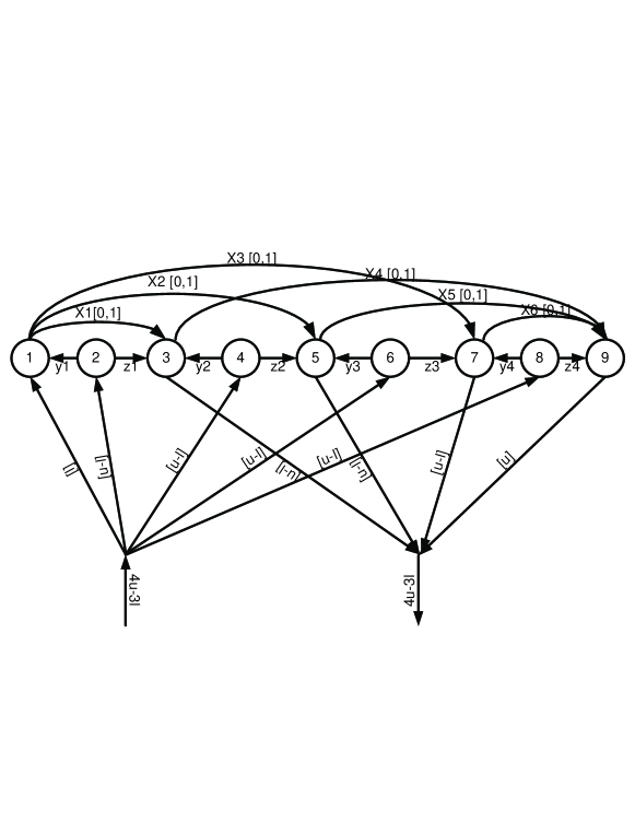
Figure 1: A flow graph for $\mbox{\sc Sequence}(l,u,3,[X_{1},\ldots,X_{6}],v)$

Theorem 4.1

For any constraint $\mbox{\sc Sequence}(l,u,k,[X_{1},\ldots,X_{n}],v)$, there is an equivalent network flow graph $G=(V,E)$ with $5n-4k+5$ edges, $2n-2k+3+2$ vertices, a maximum edge capacity of $u$, and an amount of flow to send equal to $f=(n-k)(u-l)+u$. There is a one-to-one correspondence between solutions of the constraint and feasible flows in the network.

The time complexity of finding a maximum flow of value $f$ is $O(|E|f)$ using the Ford-Fulkerson algorithm [12]. Faster algorithms exist for this problem. For example, Goldberg and Rao’s algorithm finds a maximum flow in $O(min(|V|^{2/3},|E|^{1/2})|E|\log(|V|^{2}/|E|+2)\log C)$ time where $C$ is the maximum capacity upper bound for an edge [13]. In our case, this gives $O(n^{3/2}\log n\log u)$ time complexity. We follow Régin [1, 2] in the building of an incremental filtering algorithm from the network flow formulation. A feasible flow in the graph gives us a support for one value in each variable domain. Suppose $X_{k}=v$ is in the solution that corresponds to the feasible flow where $v$ is either zero or one. To obtain a support for $X_{k}=1-v$, we find the SCC of the residual graph and check if both ends of the edge labeled with $X_{k}$ are in the same strongly connected component. If so, $X_{k}=1-v$ has a support; otherwise $1-v$ can be removed from the domain of $X_{k}$. Strongly connected components can be found in linear time, because the number of nodes and edges in the flow network for the Sequence constraint is linear in $n$ by Theorem 4.1. The total time complexity for initially enforcing DC is $O(n((n-k)(u-l)+u))$ if we use the Ford-Fulkerson algorithm or $O(n^{3/2}\log n\log u)$ if we use Goldberg and Rao’s algorithm.

Still following Régin [1, 2], one can make the algorithm incremental. Suppose during search $X_{i}$ is fixed to value $v$. If the last computed flow was a support for $X_{i}=v$, then there is no need to recompute the flow. We simply need to recompute the SCC in the new residual graph and enforce DC in $O(n)$ time. If the last computed flow is not a support for $X_{i}=v$, we can find a cycle in the residual graph containing the edge associated to $X_{i}$ in $O(n)$ time. By pushing a unit of flow over this cycle, we obtain a flow that is a support for $X_{i}=v$. Enforcing DC can be done in $O(n)$ after computing the SCC. Consequently, there is an incremental cost of $O(n)$ when a variable is fixed, and the cost of enforcing DC down a branch of the search tree is $O(n^{2})$.

5 Soft Sequence  Constraint

Soft forms of the Sequence constraint may be useful in practice. The ROADEF 2005 challenge [14], which was proposed and sponsored by Renault, puts forward a violation measure for the Sequence constraint which takes into account by how much each Among constraint is violated. We therefore consider the soft global constraint, $\mbox{\sc SoftSequence}(l,u,k,T,[X_{1},\ldots,X_{n}],v)$. This holds iff:

$$T \geq \sum_{i=1}^{n-k+1}\mbox{\rm max}(l-\sum_{j=0}^{k-1}(X_{i+j}\in v),\sum_{j=0}^{k-1}(X_{i+j}\in v)-u,0)$$ (1)

As before, we can simplify notation and consider SoftSequence on 0/1 variables and $v=\{1\}$.

We again convert to a flow problem by means of a linear program, but this time with an objective function. Consider $\mbox{\sc SoftSequence}(l,u,3,T,[X_{1},\ldots,X_{6}],v)$. We introduce variables, $Q_{i}$ and $P_{i}$ to represent the penalties that may arise from violating lower and upper bounds respectively. We can then express this SoftSequence constraint as follows. The objective function gives a lower bound on $T$.

$${\rm Minimize}\sum_{i=1}^{4}(P_{i}+Q_{i}) {\rm subject}\ {\rm to:}$$

$$X_{1}+X_{2}+X_{3}-Y_{1}+Q_{1}=l, X_{1}+X_{2}+X_{3}+Z_{1}-P_{1}=u,$$

$$X_{2}+X_{3}+X_{4}-Y_{2}+Q_{2}=l, X_{2}+X_{3}+X_{4}+Z_{2}-P_{2}=u,$$

$$X_{3}+X_{4}+X_{5}-Y_{3}+Q_{3}=l, X_{3}+X_{4}+X_{5}+Z_{3}-P_{3}=u,$$

$$X_{4}+X_{5}+X_{6}-Y_{4}+Q_{4}=l, X_{4}+X_{5}+X_{6}+Z_{3}-P_{4}=u$$

where $Y_{i}$, $Z_{i}$, $P_{i}$ and $Q_{i}$ are non-negative. In matrix form, this is:

Minimize $$\sum_{i=1}^{4}(P_{i}+Q_{i})$$    subject  to:

If we transform the matrix as before, we get a minimum cost network flow problem:

Minimize $$\sum_{i=1}^{4}(P_{i}+Q_{i})$$    subject  to:

The flow graph $G=(V,E)$ for this system is presented in Figure 2. Dashed edges have cost $1$, while other edges have cost $0$. The minimal cost flow in the graph corresponds to a minimal cost solution to the system of equations

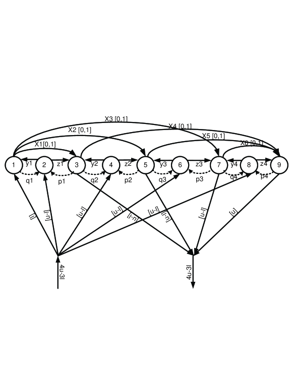
Figure 2: A flow graph for $\mbox{\sc SoftSequence}(l,u,3,T,[X_{1},\ldots,X_{6}])$

Theorem 5.1

For any constraint $\mbox{\sc SoftSequence}(l,u,k,T,[X_{1},\ldots,X_{n}],v)$, there is an equivalent network flow graph. There is a one-to-one correspondence between solutions of the constraint and feasible flows of cost less than or equal to $max(dom(T))$.

Using Theorem 5.1, we construct a DC filtering algorithm for the SoftSequence constraint. The SoftSequence constraint is DC iff the following conditions hold:

• value $1$ belongs to $dom(X_{i})$, $i=1,\ldots,n$ iff there exists a feasible flow of cost at most $\max({dom}(T))$ that sends a unit flow through the edge labeled with $X_{i}$.

• value $0$ belongs to $dom(X_{i})$, $i=1,\ldots,n$ iff there exists a feasible flow of cost at most $\max({dom}(T))$ that does not send any flow through the edge labeled with $X_{i}$.

• there exists a feasible flow of cost at most $\min({dom}(T))$.

The minimal cost flow can be found in $O(|V||E|\log\log U\log|V|C)=O(n^{2}\log n\log\log u)$ time [3]. Consider the edge $(u,v)$ in the residual graph associated to variable $X_{i}$ and let $k_{(u,v)}$ be its residual cost. If the flow corresponds to an assignment with $X_{i}=0$, pushing a unit of flow on $(u,v)$ results in a solution with $X_{i}=1$. Symmetrically, if the flow corresponds to an assignment with $X_{i}=1$, pushing a unit of flow on $(u,v)$ results in a solution with $X_{i}=0$. If the shortest path in the residual graph between $v$ and $u$ is $k_{(v,u)}$, then the shortest cycle that contains $(u,v)$ has length $k_{(u,v)}+k_{(v,u)}$. Pushing a unit of flow through this cycle results in a flow of cost $c+k_{(u,v)}+k_{(v,u)}$ which is the minimum-cost flow that contains the edge $(u,v)$. If $c+k_{(u,v)}+k_{(v,u)}>\max({dom}(T))$, then no flows containing the edge $(u,v)$ exist with a cost smaller or equal to $\max({dom}(T))$. The variable $X_{i}$ must therefore be fixed to the value taken in the current flow. Following Equation 1, the cost of the variable $T$ must be no smaller than the cost of the solution. To enforce BC on the cost variable, we increase the lower bound of ${dom}(T)$ to the cost of the minimum flow in the graph $G$.

To enforce DC on the $X$ variables efficiently we can use an all pairs shortest path algorithm on the residual graph [15]. This takes $O(n^{2}\log n)$ time using Johnson’s algorithm [12]. This gives an $O(n^{2}\log n\log\log u)$ time complexity to enforce DC on SoftSequence. The penalty variables used for SoftSequence arise directly out of the problem description and occur naturally in the LP formulation. We could also view them as arising through the methodology of [16], where edges with costs are added to the network graph for the hard constraint to represent the softened constraint.

6 Generalized Sequence Constraint

To model real world problems, we may want to have different size or positioned windows. For example, the window size in a rostering problem may depend on whether it includes a weekend or not. An extension of the Sequence constraint proposed in  [9] is that each Among constraint can have different parameters (start position, $l$, $u$, and $k$). More precisely, $\mbox{\sc Gen-Sequence}(\vec{p_{1}},\ldots,\vec{p_{m}},[X_{1},X_{2},\ldots,X_{n}],v)$ holds iff $\mbox{\sc Among}(l_{i},u_{i},k_{i},[X_{s_{i}},\ldots,X_{s_{i}+k_{i}-1}],v)$ for $1\leq i\leq m$ where $\vec{p_{i}}=\left\langle l_{i},u_{i},k_{i},s_{i}\right\rangle$. Whilst the methods in Section 4 easily extend to allow different bounds $l$ and $u$ for each window, dealing with different windows is more difficult. In general, the matrix now does not have the consecutive ones property. It may be possible to re-order the windows to achieve the consecutive ones property. If such a re-ordering exists, it can be found and performed in $O(m+n+r)$ time, where $r$ is the number of non-zero entries in the matrix [17]. Even when re-ordering cannot achieve the consecutive ones property there may, nevertheless, be an equivalent network matrix. Bixby and Cunningham [18] give a procedure to find an equivalent network matrix, when it exists, in $O(mr)$ time. Another procedure is given in [19]. In these cases, the method in Section 4 can be applied to propagate the Gen-Sequence constraint in $O(n^{2})$ time down the branch of a search tree.

Not all Gen-Sequence constraints can be expressed as network flows. Consider the Gen-Sequence constraint with $n=5$, identical upper and lower bounds ($l$ and $u$), and 4 windows: [1,5], [2,4], [3,5], and [1,3]. We can express it as an integer linear program:

$$\left(\begin{smallmatrix}1&1&1&1&1\\ -1&-1&-1&-1&-1\\ 0&1&1&1&0\\ 0&-1&-1&-1&0\\ 0&0&1&1&1\\ 0&0&-1&-1&-1\\ 1&1&1&0&0\\ -1&-1&-1&0&0\end{smallmatrix}\right)\left(\begin{smallmatrix}X_{1}\\ X_{2}\\ X_{3}\\ X_{4}\\ X_{5}\end{smallmatrix}\right)\geq\left(\begin{smallmatrix}l\\ -u\\ l\\ -u\\ l\\ -u\\ l\\ -u\end{smallmatrix}\right)$$ (2)

Applying the test described in Section 20.1 of [19] to Example 2, we find that the matrix of this problem is not equivalent to any network matrix.

However, all Gen-Sequence constraint matrices satisfy the weaker property of total unimodularity. A matrix is totally unimodular iff every square non-singular submatrix has a determinant of $+1$ or $-1$. The advantage of this property is that any totally unimodular system of inequalities with integral constants is solvable in $\mathbb{Z}$ iff it is solvable in $\mathbb{R}$.

Theorem 6.1

The matrix of the inequalities associated with Gen-Sequence constraint is totally unimodular.

In practice, only integral values for the bounds $l_{i}$ and $u_{i}$ are used. Thus the consistency of a Gen-Sequence constraint can be determined via interior point algorithms for LP in $O(n^{3.5}\log u)$ time. Using the failed literal test, we can enforce DC at a cost of $O(n^{5.5}\log u)$ down the branch of a search tree for any Gen-Sequence constraint. This is too expensive to be practical. We can, instead, exploit the fact that the matrix for each Gen-Sequence constraint has the consecutive ones property for rows (before the introduction of slack/surplus variables). Corresponding to the row transformation for matrices with consecutive ones for columns is a change-of-variables transformation into variable $S_{j}=\sum_{i=1}^{j}X_{i}$ for matrices with consecutive ones for rows. This gives the dual of a network matrix. This is the basis of an encoding of Sequence in [10] (denoted there $CD$). Consequently that encoding extends to Gen-Sequence. Adapting the analysis in [10] to Gen-Sequence, we can enforce DC in $O(nm+n^{2}\log n)$ time down the branch of a search tree.

In summary, for a compilation cost of $O(mr)$, we can enforce DC on a Gen-Sequence constraint in $O(n^{2})$ down the branch of a search tree, when it has a flow representation, and in $O(nm+n^{2}\log n)$ when it does not.

7 A SlidingSum Constraint

The SlidingSum constraint [20] is a generalization of the Sequence constraint from Boolean to integer variables, which we extend to allow arbitrary windows. SlidingSum $([X_{1},\ldots,X_{n}],[\vec{p_{1}},\ldots,\vec{p_{m}}])$ holds iff $l_{i}\leq\sum_{j=s_{i}}^{s_{i}+k_{i}-1}X_{i}\leq u_{i}$ holds where $\vec{p_{i}}=\left\langle l_{i},u_{i},k_{i},s_{i}\right\rangle$ is, as with the generalized Sequence, a window. The constraint can be expressed as a linear program $\mathcal{P}$ called the primal where $W$ is a matrix encoding the inequalities. Since the constraint represents a satisfaction problem, we minimize the constant 0. The dual $\mathcal{D}$ is however an optimization problem.

$$\left.\begin{aligned} \min\;0\\ \begin{bmatrix}W\\ -W\\ I\\ -I\end{bmatrix}X&\geq\begin{bmatrix}l\\ -u\\ a\\ -b\end{bmatrix}\end{aligned}\hskip 14.22636pt\right\}\mathcal{P} \left.\begin{aligned} \min\begin{bmatrix}-l&u&-a&b\end{bmatrix}Y\\ \begin{bmatrix}W^{T}&-W^{T}&I&-I\end{bmatrix}Y&=0\\ Y&\geq 0\end{aligned}\hskip 14.22636pt\right\}\mathcal{D}$$ (3)

Von Neumann’s Strong Duality Theorem states that if the primal and the dual problems are feasible, then they have the same objective value. Moreover, if the primal is unsatisfiable, the dual is unbounded. The SlidingSum constraint is thus satisfiable if the objective function of the dual problem is zero. It is unsatisfiable if it tends to negative infinity.

Note that the matrix $W^{T}$ has the consecutive ones property on the columns. The dual problem can thus be converted to a network flow using the same transformation as with the Sequence constraint. Consider the dual LP of our running example:

Minimize $$-\sum_{i=1}^{4}l_{i}Y_{i}+\sum_{i=1}^{4}u_{i}Y_{4+i}-\sum_{i=1}^{5}a_{i}Y_{8+i}+\sum_{i=1}^{5}b_{i}Y_{13+i}$$    subject  to:

Our usual transformation will turn this into a network flow problem:

Minimize $$-\sum_{i=1}^{4}l_{i}Y_{i}+\sum_{i=1}^{4}u_{i}Y_{4+i}-\sum_{i=1}^{5}a_{i}Y_{8+i}+\sum_{i=1}^{5}b_{i}Y_{13+i}$$    subject  to:

The flow associated with this example is given in Figure 3. There are $n+1$ nodes labelled from 1 to $n+1$ where node $i$ is connected to node $i+1$ with an edge of cost $-a_{i}$ and node $i+1$ is connected to node $i$ with an edge of cost $b_{i}$. For each window $\vec{p_{i}}$, we have an edge from $s_{i}$ to $s_{i}+k_{i}$ with cost $-l_{i}$ and an edge from $s_{i}+k_{i}$ to $s_{i}$ with cost $u_{i}$. All nodes have a null supply and a null demand. A flow is therefore simply a circulation i.e., an amount of flow pushed on the cycles of the graph.

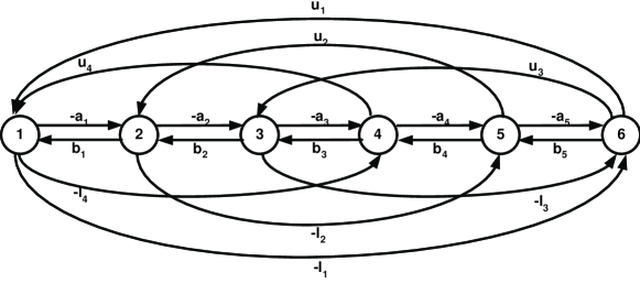
Figure 3: Network flow associated to the SlidingSum constraint posted on the running example.

Theorem 7.1

The SlidingSum constraint is satisfiable if and only there are no negative cycles in the flow graph associated with the dual linear program.

Proof

If there is a negative cycle in the graph, then we can push an infinite amount of flow resulting in a cost infinitely small. Hence the dual problem is unbounded, and the primal is unsatisfiable. Suppose that there are no negative cycles in the graph. Pushing any amount of flow over a cycle of positive cost results in a flow of cost greater than zero. Such a flow is not optimal since the null flow has a smaller objective value. Pushing any amount of flow over a null cycle does not change the objective value. Therefore the null flow is an optimal solution and since this solution is bounded, then the primal is satisfiable. Note that the objective value of the dual (zero) is in this case equal to the objective value of the primal. ∎

Based on Theorem 7.1 we build a BC filtering algorithm for the SlidingSum constraint. The SlidingSum constraint is BC iff the following conditions hold:

• value $a_{i}$ is the lower bound of a variable $X_{i}$, $i=1,\ldots,n$ iff $a_{i}$ is the smallest value in the domain of $X_{i}$ such that there are no negative cycles through the edge weighted with $-a_{i}$ and labeled with the lower bound of $X_{i}$.

• value $b_{i}$ is the upper bound of a variable $X_{i}$, $i=1,\ldots,n$ iff $b_{i}$ is the greatest value in the domain of $X_{i}$ such that there are no negative cycles through the edge weighted with $b_{i}$ and labeled with the upper bound of $X_{i}$

The flow graph has $O(n)$ nodes and $O(n+m)$ edges. Testing whether there is a negative cycle takes $O(n^{2}+nm)$ time using the Bellman-Ford algorithm. We find for each variable $X_{i}$ the smallest (largest) value in its domain such that assigning this value to $X_{i}$ does not create a negative cycle. We compute the shortest path between all pairs of nodes using Johnson’s algorithm in $O(|V|^{2}\log|V|+|V||E|)$ time which in our case gives $O(n^{2}\log n+nm)$ time. Suppose that the shortest path between $i$ and $i+1$ has length $s(i,i+1)$, then for the constraint to be satisfiable, we need $b_{i}+s(i,i+1)\geq 0$. Since $b_{i}$ is a value potentially taken by $X_{i}$, we need to have $X_{i}\geq-s(i,i+1)$. We therefore assign $\min({dom}(X_{i}))\leftarrow\max(\min({dom}(X_{i})),-s(i,i+1))$. Similarly, let the length of the shortest path between $i+1$ and $i$ be $s(i+1,i)$. For the constraint to be satisfiable, we need $s(i+1,i)-a_{i}\geq 0$. Since $a_{i}$ is a value potentially taken by $X_{i}$, we have $X_{i}\leq s(i+1,i)$. We assign $\max(X_{i})\leftarrow\min(\max(X_{i}),s(i+1,i))$. It is not hard to prove this is sound and complete, removing all values that cause negative cycles. Following [10], we can make the propagator incremental using the algorithm by Cotton and Maler [21] to maintain the shortest path between $|P|$ pairs of nodes in $O(|E|+|V|\log|V|+|P|)$ time upon edge reduction. Each time a lower bound $a_{i}$ is increased or an upper bound $b_{i}$ is decreased, the shortest paths can be recomputed in $O(m+n\log n)$ time.

8 Experimental Results

To evaluate the performance of our filtering algorithms we carried out a series of experiments on random problems. The experimental setup is similar to that in [10]. The first set of experiments compares performance of the flow-based propagator $FB$ on single instance of the Sequence constraint against the $HPRS$ propagator (the third propagator in [9]), the $CS$ encoding of [10], and the Among decomposition ($AD$) of Sequence. The second set of experiments compares the flow-based propagator $FB_{S}$ for the SoftSequence constraint and its decomposition into soft Among constraints. Experiments were run with ILOG 6.1 on an Intel Xeon 4 CPU, 2.0 Ghz, 4G RAM. Boost graph library version $1.34.1$ was used to implement the flow-based algorithms.

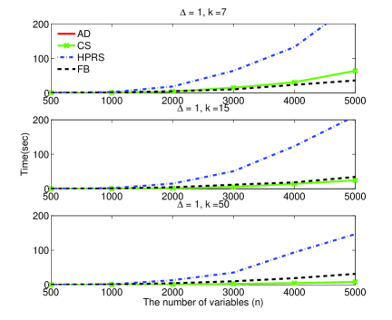
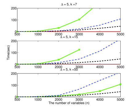
Figure 4: Randomly generated instances with a single Sequence constraints for different combinations of $\Delta$ and $k$.

8.1 The Sequence constraint

For each possible combination of $n\in\{500,1000,2000,3000,4000,5000\}$, $k\in\{5,15,50\}$, $\Delta=u-l\in\{1,5\}$, we generated twenty instances with random lower bounds in the interval $(0,k-\Delta)$. We used random value and variable ordering and a time out of $300$ sec. We used the Ford-Fulkerson algorithm to find a maximum flow. Results for different values of $\Delta$ are presented in Tables 1, 2 and Figure 4. Table 1 shows results for tight problems with $\Delta=1$ and Table 2 for easy problems with $\Delta=5$. To investiage empirically the asymptotic growth of the different propagators, we plot average time to solve 20 instances against the instance size for each combination of parameters $k$ and $\Delta$ in Figure 4. First of all, we notice that the $CS$ encoding is the best on hard instances ($\Delta=1$) and the $AD$ decomposition is the fastest on easy instances ($\Delta=5$). This result was first observed in  [10]. The $FB$ propagator is not the fastest one but has the most robust performance. It is sensitive only to the value of $n$ and not to other parameters, like the length of the window($k$) or hardness of the problem($\Delta$). As can be seen from Figure 4, the $FB$ propagator scales better than the other propagators with the size of the problem. It appears to grow linearly with the number of variables, while the $HPRS$ propagator display quadratic growth.

Table 1: Randomly generated instances with a single Sequence constraint and $\Delta=1$. Number of instances solved in 300 sec / average time to solve. We omit results for $n\in\{1000,3000,4000\}$ due to space limitation. The summary rows include all instances.

$n$	$k$	$AD$		$CS$		$HPRS$		$FB$
500	7	8	/ 2.13	20	/ 0.13	20	/ 0.35	20	/ 0.30
	15	6	/ 0.01	20	/ 0.09	20	/ 0.30	20	/ 0.29
	50	2	/ 0.02	20	/ 0.07	20	/ 0.26	20	/ 0.28
2000	7	4	/ 0.04	20	/ 4.25	20	/ 18.52	20	/ 4.76
	15	0	/0	20	/ 1.84	20	/ 15.19	20	/ 4.56
	50	1	/0	20	/ 1.16	20	/ 13.24	20	/ 4.42
5000	7	1	/0	20	/ 64.05	15	/ 262.17	20	/ 36.09
	15	0	/0	20	/ 24.46	17	/ 211.17	20	/ 34.59
	50	0	/0	20	/ 8.24	19	/ 146.63	20	/ 31.66
TOTALS
solved/total		37	/360	360	/360	351	/360	360	/360
avg time for solved		0.517		9.943		60.973		11.874
avg bt for solved		17761		429		0		0

Table 2: Randomly generated instances with a single Sequence constraint and $\Delta=5$. Number of instances solved in 300 sec / average time to solve. We omit results for $n\in\{1000,3000,4000\}$ due to space limitation. The summary rows include all instances.

$n$	$k$	$AD$		$CS$		$HPRS$		$FB$
500	7	20	/ 0.01	20	/ 0.58	20	/ 0.15	20	/ 0.44
	15	20	/ 0.01	20	/ 0.69	20	/ 0.25	20	/ 0.44
	50	18	/ 0.02	20	/ 0.20	20	/ 0.37	20	/ 0.42
2000	7	20	/ 0.07	20	/ 32.41	20	/ 7.19	20	/ 6.62
	15	20	/ 0.07	20	/ 39.71	20	/ 14.89	20	/ 6.63
	50	5	/ 5.19	20	/ 9.52	20	/ 13.71	20	/ 6.94
5000	7	20	/ 0.36	0	/0	20	/ 109.18	20	/ 46.42
	15	20	/ 0.36	6	/ 160.99	17	/ 215.97	20	/ 45.97
	50	9	/ 0.48	20	/ 108.34	11	/ 210.53	20	/ 44.88
TOTALS
solved/total		296	/360	308	/360	345	/360	360	/360
avg time for solved		0.236		52.708		50.698		16.200
avg bt for solved		888		1053		0		0

8.2 The Soft Sequence constraint

We evaluated performance of the soft Sequence constraint on random problems. For each possible combination of $n\in\{50,100\}$, $k\in\{5,15,25\}$, $\Delta=\{1,5\}$ and $m\in\{4\}$ (where $m$ is the number of Sequence constraints), we generated twenty random instances. All variables had domains of size 5. An instance was obtained by selecting random lower bounds in the interval $(0,k-\Delta)$. We excluded instances where $\sum_{i=1}^{m}l_{i}\geq k$ to avoid unsatisfiable instances. We used a random variable and value ordering, and a time-out of $300$ sec. All Sequence constraints were enforced on disjoint sets of cardinality one. Instances with $\Delta=1$ are hard instances for Sequence propagators [10], so that any DC propagator could solve only few instances. Instances with $\Delta=5$ are much looser problems, but they are still hard do solve because each instance includes four overlapping Sequence constraints. To relax these instances, we allow the Sequence constraint to be violated with a cost that has to be less than or equal to $15\%$ of the length of the sequence. Experimental results are presented in Table 3. As can be seen from the table, the $FB_{S}$ algorithms is competitive with the decomposition into soft Among constraints on relatively easy problems and outperforms the decomposition on hard problems in terms of the number of solved problems.

We observed that the flow-based propagator for the SoftSequence constraint ($FB_{S}$) is very slow. Note that the number of backtracks of $FB_{S}$ is three order of magnitudes smaller compared to $AD_{S}$. We profiled the algorithm and found that it spends most of the time performing the all pairs shortest path algorithm. Unfortunately, this is difficult to compute incrementally because the residual graph can be different on every invocation of the propagator.

Table 3: Randomly generated instances with 4 soft Sequences. Number of instances solved in 300 sec / average time to solve.

		$\Delta=1$				$\Delta=5$
$n$	$k$	$AD_{S}$		$FB_{S}$		$AD_{S}$		$FB_{S}$
50	7	6	/ 19.30	7	/ 27.91	20	/ 0.01	20	/ 2.17
	15	8	/ 36.07	13	/ 20.41	11	/ 49.49	10	/ 30.51
	25	6	/ 0.73	10	/ 23.27	10	/ 6.40	10	/ 7.41
100	7	1	/0	3	/ 7.56	19	/ 10.50	18	/ 16.51
	15	0	/0	5	/ 6.90	3	/ 0.01	3	/ 7.20
	25	0	/0	5	/ 4.96	5	/ 19.07	5	/ 23.99
TOTALS
solved/total		21	/120	43	/120	68	/120	66	/120
avg time for solved		19.463		18.034		13.286		13.051
avg bt for solved		245245		343		147434		128

9 Conclusion

We have proposed new filtering algorithms for the Sequence constraint and several extensions including the soft Sequence and generalized Sequence constraints which are based on network flows. Our propagator for the Sequence constraint enforces domain consistency in $O(n^{2})$ time down a branch of the search tree. This improves upon the best existing domain consistency algorithm by a factor of $O(\log n)$. We also introduced a soft version of the Sequence constraint and propose an $O(n^{2}\log n\log\log u)$ time domain consistency algorithm based on minimum cost network flows. These algorithms are derived from linear programs which represent a network flow. They differ from the flows used to propagate global constraints like Gcc since the domains of the variables are encoded as costs on the edges rather than capacities. Such flows are efficient for maintaining bounds consistency over large domains. Experimental results demonstrate that the $FB$ filtering algorithm is more robust than existing propagators. We conjecture that similar flow based propagators derived from linear programs may be useful for other global constraints.

References

- [1] Régin, J.C.: A filtering algorithm for constraints of difference in csps. In: Proc. of the 12th National Conf. on AI (AAAI’94). Volume 1. (1994) 362–367
- [2] Régin, J.C.: Generalized arc consistency for global cardinality constraint. In: Proc. of the 12th National Conf. on AI (AAAI’96). (1996) 209–215
- [3] Ahuja, R.K., Magnanti, T.L., Orlin, J.B.: Network Flows: Theory, Algorithms, and Applications. Prentice Hall (1993)
- [4] Beldiceanu, N., Contejean, E.: Introducing global constraints in CHIP. Mathematical and Computer Modelling 12 (1994) 97–123
- [5] Bessiere, C., Hebrard, E., Hnich, B., Kiziltan, Z., Walsh, T.: The slide meta-constraint. Technical report (2007)
- [6] Régin, J.C., Puget, J.F.: A filtering algorithm for global sequencing constraints. In: Proc. of the 3th Int. Conf. on Principles and Practice of Constraint Programming. (1997) 32–46
- [7] Beldiceanu, N., Carlsson, M.: Revisiting the cardinality operator and introducing cardinality-path constraint family. In: Proc. of the Int. Conf. on Logic Programming. (2001) 59–73
- [8] Régin, J.C.: Combination of among and cardinality constraints. In: Integration of AI and OR Techniques in Constraint Programming for Combinatorial Optimization Problems, Second International Conference. Volume 3524., Springer (2005) 288–303
- [9] Hoeve, W.J.v., Pesant, G., Rousseau, L.M., Sabharwal, A.: Revisiting the sequence constraint. In: Proc. of the 12th Int. Conf. on Principles and Practice of Constraint Programming. (2006) 620–634
- [10] Brand, S., Narodytska, N., Quimper, C.G., Stuckey, P., Walsh, T.: Encodings of the sequence constraint. In: Proc. of the 13th Int. Conf. on Principles and Practices of Constraint Programming. Volume 4741. (2007) 210–224
- [11] A.F. Veinott, J., Wagner, H.: Optimal capacity scheduling I. Operations Research 10(4) (1962) 518–532
- [12] Cormen, T.H., Leiserson, C.E., Rivest, R.L., Stein, C.: Introduction to Algorithms, Second Edition. The MIT Press (2001)
- [13] Goldberg, A.V., Rao, S.: Beyond the flow decomposition barrier. J. ACM 45 (1998) 753–782
- [14] Solnon, C., Cung, V.D., Nguyen, A., Artigues, C.: The car sequencing problem: overview of state-of-the-art methods and industrial case-study of the ROADEF’2005 challenge problem. European Journal of Operational Research (EJOR) (2008) In press.
- [15] Régin, J.C.: Arc consistency for global cardinality constraints with costs. In: Proceedings of the 5th International Conference on Principles and Practice of Constraint Programming (CP ’99), Springer-Verlag (1999) 390–404
- [16] van Hoeve, W.J., Pesant, G., Rousseau, L.M.: On global warming: Flow-based soft global constraints. J. Heuristics 12(4-5) (2006) 347–373
- [17] Booth, K., Lueker, G.: Testing for the consecutive ones property, interval graphs and graph planarity using PQ-tree algorithms. Journal of Computer and Systems Sciences 13 (1976) 335–379
- [18] Bixby, R., Cunningham, W.: Converting linear programs to network problems. Mathematics of Operations Research 5 (1980) 321–357
- [19] Schrijver, A.: Theory of linear and integer programming. John Wiley & Sons, Inc. (1986)
- [20] Beldiceanu, N.: Global constraint catalog. T-2005-08, SICS Technical Report (2005)
- [21] Cotton, S., Maler, O.: Fast and flexible difference constraint propagation for DPLL(T). In: Proc. of Theory and Applications of Satisfiability Testing (SAT-2006). (2006) 170–183