Elicitation strategies for fuzzy constraint problems with missing preferences: algorithms and experimental studies

Abstract

Fuzzy constraints are a popular approach to handle preferences and over-constrained problems in scenarios where one needs to be cautious, such as in medical or space applications. We consider here fuzzy constraint problems where some of the preferences may be missing. This models, for example, settings where agents are distributed and have privacy issues, or where there is an ongoing preference elicitation process. In this setting, we study how to find a solution which is optimal irrespective of the missing preferences. In the process of finding such a solution, we may elicit preferences from the user if necessary. However, our goal is to ask the user as little as possible. We define a combined solving and preference elicitation scheme with a large number of different instantiations, each corresponding to a concrete algorithm which we compare experimentally. We compute both the number of elicited preferences and the ”user effort”, which may be larger, as it contains all the preference values the user has to compute to be able to respond to the elicitation requests. While the number of elicited preferences is important when the concern is to communicate as little information as possible, the user effort measures also the hidden work the user has to do to be able to communicate the elicited preferences. Our experimental results show that some of our algorithms are very good at finding a necessarily optimal solution while asking the user for only a very small fraction of the missing preferences. The user effort is also very small for the best algorithms. Finally, we test these algorithms on hard constraint problems with possibly missing constraints, where the aim is to find feasible solutions irrespective of the missing constraints.

1 Introduction

Constraint programming is a powerful paradigm for solving scheduling, planning, and resource allocation problems. A problem is represented by a set of variables, each with a domain of values, and a set of constraints. A solution is an assignment of values to the variables which satisfies all constraints and which optionally maximizes/minimizes an objective function. Soft constraints are a way to model optimization problems by allowing for several levels of satisfiability, modelled by the use of preference or cost values that represent how much we like an instantiation of the variables of a constraint.

It is usually assumed that the data (variables, domains, (soft) constraints) is completely known before solving starts. This is often unrealistic. In web applications and multi-agent systems, the data is frequently only partially known and may be added to at a later date by, for example, elicitation. Data may also come from different sources at different times. In multi-agent systems, agents may release data reluctantly due to privacy concerns.

Incomplete soft constraint problems can model such situations by allowing some of the preferences to be missing. An algorithm has been proposed and tested to solve such incomplete problems [7]. The goal is to find a solution that is guaranteed to be optimal irrespective of the missing preferences, eliciting preferences if necessary until such a solution exists. Two notions of optimal solution are considered: possibly optimal solutions are assignments that are optimal in at least one way of revealing the unspecified preferences, while necessarily optimal solutions are assignments that are optimal in all ways that the unspecified preferences can be revealed. The set of possibly optimal solutions is never empty, while the set of necessarily optimal solutions can be empty.

If there is no necessarily optimal solution, the algorithm proposed in [7] uses branch and bound to find a ”promising solution” (specifically, a complete assignment in the best possible completion of the current problem) and elicits the missing preferences related to this assignment. This process is repeated till there is a necessarily optimal solution.

Although this algorithm behaves reasonably well, it make some specific choices about solving and preference elicitation that may not be optimal in practice, as we shall see in this paper. For example, the algorithm only elicits missing preferences after running branch and bound to exhaustion. As a second example, the algorithm elicits all missing preferences related to the candidate solution. Many other strategies are possible. We might elicit preferences at the end of every complete branch, or even at every node in the search tree. Also, when choosing the value to assign to a variable, we might ask the user (who knows the missing preferences) for help. Finally, we might not elicit all the missing preferences related to the current candidate solution. For example, we might just ask the user for the worst preference among the missing ones.

In this paper we consider a general algorithm scheme which greatly generalizes that proposed in [7]. It is based on three parameters: what to elicit, when to elicit it, and who chooses the value to be assigned to the next variable. We test all 16 possible different instances of the scheme (among which is the algorithm in [7]) on randomly generated fuzzy constraint problems. We demonstrate that some of the algorithms are very good at finding necessarily optimal solution without eliciting too many preferences. We also test the algorithms on problems with hard constraints. Finally, we consider problems with fuzzy temporal constraints, where problems have more specific structure.

In our experiments, we compute the elicited preferences, that is, the missing values that the user has to provide to the system because they are requested by the algorithm. Providing these values usually has a cost, either in terms of computation effort, or in terms of privacy decrease, or also in terms of communication bandwidth. Thus knowing how many preferences are elicited is important if we care about any of these issues. However, we also compute a measure of the user’s effort, which may be larger than the number of elicited preferences, as it contains all the preference values the user has to consider to be able to respond to the elicitation requests. For example, we may ask the user for the worst preference value among $k$ missing ones: the user will communicate only one value, but he will have to consider all $k$ of them. While knowing the number of elicited preferences is important when the concern is to communicate as little information as possible, the user effort measures also the hidden work the user has to do to be able to communicate the elicited preferences. This user’s effort is therefore also an important measure.

As a motivating example, recommender systems give suggestions based on partial knowledge of the user’s preferences. Our approach could improve performance by identifying some key questions to ask before giving recommendations. Privacy concerns regarding the percentage of elicited preferences are motivated by eavesdropping. User’s effort is instead related to the burden on the user.

Our results show that the choice of preference elicitation strategy is crucial for the performance of the solver. While the best algorithms need to elicit as little as 10% of the missing preferences, the worst one needs much more. The user’s effort is also very small for the best algorithms. The performance of the best algorithms shows that we only need to ask the user a very small amount of additional information to be able to solve problems with missing data.

Several other approaches have addressed similar issues. For example, open CSPs [4, 6] and interactive CSPs [9] work with domains that can be partially specified. As a second example, in dynamic CSPs [2] variables, domains, and constraints may change over time. However, the incompleteness considered in [6, 5] is on domain values as well as on their preferences. Working under this assumption means that the agent that provides new values/costs for a variable knows all possible costs, since they are capable of providing the best value first. If the cost computation is expensive or time consuming, then computing all such costs (in order to give the most preferred value) is not desirable. We assume instead, as in [7], that all values are given at the beginning, and that only some preferences are missing. Because of this assumption, we don’t need to elicit preference values in order, as in [6].

2 Background

In this section we give a brief overview of the fundamental notions and concepts on Soft Constraints and Incomplete Soft Constraints.

Incomplete Soft Constraints problems (ISCSPs) [7] extend Soft Constraint Problems (SCSPs) [1] to deal with partial information. We will focus on a specific instance of this framework in which the soft constraints are fuzzy.

Given a set of variables $V$ with finite domain $D$, an incomplete fuzzy constraint is a pair $\langle idef,$ $con\rangle$ where $con\subseteq V$ is the scope of the constraint and $idef:D^{|con|}\longrightarrow[0,1]\cup\{?\}$ is the preference function of the constraint associating to each tuple of assignments to the variables in $con$ either a preference value ranging between 0 and 1, or $?$. All tuples mapped into $?$ by $idef$ are called incomplete tuples, meaning that their preference is unspecified. A fuzzy constraint is an incomplete fuzzy constraint with no incomplete tuples.

An incomplete fuzzy constraint problem (IFCSP) is a pair $\langle C,V,D\rangle$ where $C$ is a set of incomplete fuzzy constraints over the variables in $V$ with domain $D$. Given an IFCSP $P$, $IT(P)$ denotes the set of all incomplete tuples in $P$. When there are no incomplete tuples, we will denote a fuzzy constraint problem by FSCP.

Given an IFCSP $P$, a completion of $P$ is an IFCSP $P^{\prime}$ obtained from $P$ by associating to each incomplete tuple in every constraint an element in $[0,1]$. A completion is partial if some preference remains unspecified. $C(P)$ denotes the set of all possible completions of $P$ and $PC(P)$ denotes the set of all its partial completions.

Given an assignment $s$ to all the variables of an IFCSP $P$, $pref(P,s)$ is the preference of $s$ in $P$, defined as $pref(P,s)=min_{<idef,con>\in C|idef(s_{\downarrow con})\neq?}idef(s_{\downarrow con})$. It is obtained by taking the minimum among the known preferences associated to the projections of the assignment, that is, of the appropriated sub-tuples in the constraints.

In the fuzzy context, a complete assignment of values to all the variables is an optimal solution if its preference is maximal. The optimality notion of FCSPs is generalized to IFCSPs via the notions of necessarily and possibly optimal solutions, that is, complete assignments which are maximal in all or some completions. Given an IFCSP $P$, we denote by $NOS(P)$ (resp., $POS(P)$) the set of necessarily (resp., possibly) optimal solutions of $P$. Notice that $NOS(P)\subseteq POS(P)$. Moreover, while $POS(P)$ is never empty, $NOS(P)$ may be empty. In particular, $NOS(P)$ is empty whenever the revealed preferences do not fix the relationship between one assignment and all others.

In [7] an algorithm is proposed to find a necessarily optimal solution of an IFCSP based on a characterization of $NOS(P)$ and $POS(P)$. This characterization uses the preferences of the optimal solutions of two special completions of $P$, namely the ${\bf 0}$-completion of $P$, denoted by $P_{0}$, obtained from $P$ by associating preference $0$ to each tuple of $IT(P)$, and the ${\bf 1}$-completion of $P$, denoted by $P_{1}$, obtained from $P$ by associating preference $1$ to each tuple of $IT(P)$. Notice that, by monotonicity of $min$, we have that $pref_{0}\leq pref_{1}$. When $pref_{0}=pref_{1}$, $NOS(P)=Opt(P_{0})$; thus, any optimal solution of $P_{0}$ is a necessary optimal solution. Otherwise, $NOS(P)$ is empty and $POS(P)$ is a set of solutions with preference between $pref_{0}$ and $pref_{1}$ in $P_{1}$. The algorithm proposed in [7] finds a necessarily optimal solution of the given IFCSP by interleaving the computation of $pref_{0}$ and $pref_{1}$ with preference elicitation steps, until the two values coincide. Moreover, the preference elicitation is guided by the fact that only solutions in $POS(P)$ can become necessarily optimal. Thus, the algorithm only elicits preferences related to optimal solutions of $P_{1}$.

3 A general solver scheme

We now propose a more general schema for solving IFCSPs based on interleaving branch and bound (BB) search with elicitation. This schema generalizes the concrete solver presented in [7], but has several other instantiations that we will consider and compare experimentally in this paper. The scheme uses branch and bound. This considers the variables in some order, choosing a value for each variable, and pruning branches based on an upper bound (assuming the goal is to maximize) on the preference value of any completion of the current partial assignment. To deal with missing preferences, branch and bound is applied to both the 0-completion and the ${\bf 1}$-completion of the problem. If they have the same solution, this is a necessarily optimal solution and we can stop. If not, we elicit some of the missing preferences and continue branch and bound on the new ${\bf 1}$-completion.

Preferences can be elicited after each run of branch and bound (as in [7]) or during a BB run while preserving the correctness of the approach. For example, we can elicit preferences at the end of every complete branch (that is, regarding preferences of every complete assignment considered in the branch and bound algorithm), or at every node in the search tree (thus considering every partial assignment). Moreover, when choosing the value for the next variable to be assigned, we can ask the user (who knows the missing preferences) for help. Finally, rather than eliciting all the missing preferences in the possibly optimal solution, or the complete or partial assignment under consideration, we can elicit just one of the missing preferences. For example, with fuzzy constraint problems, eliciting just the worst preference among the missing ones is sufficient since only the worst value is important to the computation of the overall preference value. More precisely, the algorithm schema we propose is based on the following parameters:

1. Who chooses the value of a variable: the algorithm can choose the values in decreasing order either w.r.t. their preference values in the ${\bf 1}$-completion (Who=dp) or in the ${\bf 0}$-completion (Who=dpi). Otherwise, the user can suggest this choice. To do this, he can consider all the preferences (revealed or not) for the values of the current variable (lazy user, Who=lu for short); or he considers also the preference values in constraints between this variable and the past variables in the search order (smart user, Who=su for short).

2. What is elicited: we can elicit the preferences of all the incomplete tuples of the current assignment (What=all) or only the worst preference in the current assignment, if it is worse than the known ones (What=worst);

3. When elicitation takes place: we can elicit preferences at the end of the branch and bound search (When=tree), or during the search, when we have a complete assignment to all variables (When=branch) or whenever a new value is assigned to a variable (When=node).

By choosing a value for each of the three above parameters in a consistent way, we obtain in total 16 different algorithms, as summarized in Figure 1, where the circled instance is the concrete solver used in [7].

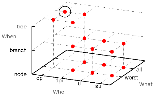
Figure 1: Instances of the general scheme.

IFCSP-SCHEME($P$,$Who$,$What$,$When$) $Q\leftarrow P_{0}$ $s_{max}$, $pref_{max}$ $\leftarrow BB(P_{0},-)$ $Q^{\prime}$,$s_{1}$,$pref_{1}$ $\leftarrow BBE(P,0,Who,What,When,s_{max},pref_{max})$ If ($s_{1}\neq nil$) $s_{max}\leftarrow s_{1}$, $pref_{max}\leftarrow pref_{1}$, $Q\leftarrow Q^{\prime}$ Return $Q$, $s_{max}$, $pref_{max}$

Figure 2: Algorithm IFCSP-SCHEME.

Figures 2 and 3 show the pseudo-code of the general scheme for solving IFCSPs. There are three algorithms: ISCSP-SCHEME, BBE and BB. ISCSP-SCHEME takes as input an IFCSP $P$ and the values for the three parameters: Who, What and When. It returns a partial completion of $P$ that has some necessarily optimal solutions, one of these necessarily optimal solutions, and its preference value. It starts by computing via branch and bound (algorithm BB) an optimal solution of $P_{0}$, say $s_{max}$, and its preference $pref_{max}$. Next, procedure $BBE$ is called. If $BBE$ succeeds, it returns a partial completion of $P$, say $Q$, one of its necessarily optimal solutions, say $s_{1}$, and its associated preference $pref_{1}$. Otherwise, it returns a solution equal to $nil$. In the first case the output of IFCSP-SCHEME coincides with that of BBE, otherwise IFCSP-SCHEME returns $P_{0}$, one of its optimal solutions, and its preference.

Procedure BBE takes as input the same values as IFCSP-SCHEME and, in addition, a solution $sol$ and a preference $lb$ representing the current lower bound on the optimal preference value. Function $nextVariable$, applied to the ${\bf 1}$-completion of the IFCSP, returns the next variable to be assigned. The algorithm then assigns a value to this variable. If the Boolean function $nextValue$ returns true (if there is a value in the domain), we select a value for $currentVar$ according to the value of parameter $Who$.

Function $UpperBound$ computes an upper bound on the preference of any completion of the current partial assignment: the minimum over the preferences of the constraints involving only variables that have already been instantiated.

If When=tree, elicitation is handled by procedure $Elicit@tree$, and takes place only at the end of the search over the ${\bf 1}$-completion. The user is not involved in the value assignment steps within the search. At the end of the search, if a solution is found, the user is asked either to reveal all the preferences of the incomplete tuples in the solution (if What=all), or only the worst one among them (if What=worst). If such a preference is better than the best found so far, BBE is called recursively with the new best solution and preference.

If When=branch, BB is performed only once. The user may be asked to choose the next value for the current variable being instantiated. Preference elicitation, which is handled by function $Elicit@branch$, takes place during search, whenever all variables have been instantiated and the user can be asked either to reveal the preferences of all the incomplete tuples in the assignment (What=all), or the worst preference among those of the incomplete tuples of the assignment (What=worst). In both cases the information gathered is sufficient to test such a preference value against the current lower bound.

If When=node, preferences are elicited every time a new value is assigned to a variable and it is handled by procedure $Elicit@node$. The tuples to be considered for elicitation are those involving the value which has just been assigned and belonging to constraints between the current variable and already instantiated variables. If What=all, the user is asked to provide the preferences of all the incomplete tuples involving the new assignment. Otherwise if What=worst, the user provides only the preference of the worst tuple.

BBE ($P$,$nInstVar$, $Who$, $What$, $When$, $sol$, $lb$) $sol^{\prime}$ $\leftarrow$ $sol$, $pref^{\prime}$ $\leftarrow$ $lb$ $currentVar\leftarrow nextVariable(P_{1})$ While ($nextValue(currentVar,Who)$) If ($When=node$) $P,pref\leftarrow Elicit@Node(What,P,currentVar,lb)$ $ub\leftarrow UpperBound(P_{1},currentVar)$ If ($ub\ >\ lb$) If ($nInstvar$ = $number\ of\ variables\ in\ P$) If ($When$ = $branch$) $P,\ pref\leftarrow Elicit@branch(What,P,lb)$ If ($pref\ >\ lb$) $sol\leftarrow getSolution(P_{1})$ $lb\leftarrow pref(P_{1},sol)$ else $BBE(P,nInstVar+1,Who,What,When,sol,lb)$ If ($When$=$tree$ $and$ $nInstVar=0$) If ($sol$ = $nil$) $sol$ $\leftarrow$ $sol^{\prime}$, $pref$ $\leftarrow$ $pref^{\prime}$ else $P,\ pref\leftarrow Elicit@tree(What,P,sol,lb)$ If ($pref>pref^{\prime}$) $BBE(P,0,Who,What,When,sol,pref)$ else $BBE(P,0,Who,What,When,sol^{\prime},pref^{\prime})$

Figure 3: Algorithm BBE.

Theorem 3.1

Given an IFCSP $P$ and a consistent set of values for parameters When, What and Who, Algorithm IFCSP-SCHEME always terminates, and returns an IFCSP $Q\in PC(P)$, an assignment $s\in NOS(Q)$, and its preference in $Q$.

Proof

Let us first notice that, as far as correctness and termination concern, the value of parameter Who is irrelevant.

We consider two separate cases, i.e., When=tree and and When=branch or node.

Case 1: When =tree.
Clearly IFCSP-SCHEME terminates if and only if BBE terminates. If we consider the pseudocode of procedure BBE shown in Algorithm 3, we see that if When = tree, BBE terminates when $sol=nil$. This happens only when the search fails to find a solution of the current problem with a preference strictly greater than the current lower bound. Let us denote with $Q^{i}$ and $Q^{i+1}$ respectively the IFCSPs given in input to the $i$-th and $i+1$-th recursive call of BBE. First we notice that only procedure $Elicit@tree$ modifies the IFCSP in input by possibly adding new elicited preferences. Moreover, whatever the value of parameter What is, the returned IFCSP is either the same as the one in input or it is a (possibly partial) completion of the one in input. Thus we have $Q^{i+1}\in PC(Q^{i})$ and $Q^{i}\in PC(P)$. Since the search is always performed on the ${\bf 1}$-completion of the current IFCSP, we can conclude that for every solution $s$, $pref(Q^{i+1},s)\leq pref(Q^{i},s)$. Let us now denote with $lb^{i}$ and $lb^{i+1}$ the lower bounds given in input respectively to the $i$-th and $i+1$-th recursive call of BBE. It is easy to see that $lb^{i+1}\geq lb^{i}$. Thus, since at every iteration we have that the preferences of solutions can only get lower, and the bound can only get higher, and since we have a finite number of solutions, we can conclude that BBE always terminates.

The reasoning that follows relies on the fact that value $pref$ returned by function $Elicit@tree$ is the final preference after elicitation of assignment $sol$ given in input. This is true since either What = all and thus all preferences have been elicited and the overall preference of $sol$ can be computed or only the worst preference has been elicited but in a fuzzy context where the overall preference coincide with the worst one. If called with When = tree IFCSP-SCHEME exits when the last branch and bound search has ended returning $sol=nil$. In such a case $sol$ and $pref$ are updated to contain the best solution and associated preference found so far, i.e., $sol^{\prime}$ and $pref^{\prime}$. Then, the algorithm returns the current IFCSP, say $Q$, and $sol$ and $pref$. Following the same reasoning as above done for $Q^{i}$ we can conclude that $Q\in PC(P)$.

At the end of every while loop execution, assignment $sol$ either contains an optimal solution $sol$ of the ${\bf 1}$-completion of the current IFCSP or $sol=nil$. $sol=nil$ iff there is no assignment with preference higher than $lb$ in the ${\bf 1}$-completion of the current IFCSP. In this situation, $sol^{\prime}$ and $pref^{\prime}$ are an optimal solution and preference of the $1$-completion of the current IFCSP. However, since the preference of $sol^{\prime}$, $pref^{\prime}$ is independent of unknown preferences and since due to monotonicity the optimal preference value of the ${\bf 1}$-completion is always greater than or equal to that of the ${\bf 0}$-completion we have that $sol^{\prime}$ and $pref^{\prime}$ are an optimal solution and preference of the ${\bf 0}$-completion of the current IFCSP as well.

By Theorems 1 and 2 of [7] we can conclude that $NOS(Q)$ is not empty. If $pref={\bf 0}$, then $NOS(Q)$ contains all the assignments and thus also $sol$. The algorithm correctly returns the same IFCSP given in input, assignment $sol$ and its preference $pref$. If instead ${\bf 0}<pref$, again the algorithm is correct, since by Theorem 1 of [7] we know that $NOS(Q)=Opt(Q_{0})$, and we have shown that $sol\in Opt(Q_{0})$.

Case 2: When=branch or node.
In order to prove that the algorithm terminates, it is sufficient to show that $BBE$ terminates. Since the domains are finite, the labeling phase produces a number of finite choices at every level of the search tree. Moreover, since the number of variables is limited, then, we have also a finite number of levels in the tree. Hence, $BBE$ considers at most all the possible assignments, that are a finite number. At the end of the execution of IFCSP-SCHEME, $sol$, with preference $pref$ is one of the optimal solutions of the current $P_{1}$Thus, for every assignment $s^{\prime}$, $pref(P_{1},s^{\prime})\leq pref(P_{1},sol)$. Moreover, for every completion $Q^{\prime}\in C(P)$ and for every assignment $s^{\prime}$, $pref(Q^{\prime},s^{\prime})\leq$ $pref(P_{1},s^{\prime})$. Hence, for every assignment $s^{\prime}$ and for every $Q^{\prime}\in C(P)$, we have that $pref(Q^{\prime},s^{\prime})\leq$ $pref(P_{1},sol)$. In order to prove that $sol\in NOS(P)$, now it is sufficient to prove that for every $Q^{\prime}\in C(P)$, $pref(P_{1},sol)=pref(Q^{\prime},sol)$. This is true, since $sol$ has a preference that is independent from the missing preferences of $P$, both when eliciting all the missing preferences, and when eliciting only the worst one either at branch or node level. In fact, in both cases, the preference of $sol$ is the same in every completion. Q.E.D.

If When=tree, then we elicit after each BB run, and it is proven in [7] that IFCSP-SCHEME never elicits preferences involved in solutions which are not possibly optimal. This is a desirable property, since only possibly optimal solutions can become necessarily optimal. However, the experiments will show that solvers satisfying such a desirable property are often out-performed in practice.

4 Problem generator and experimental design

To test the performance of these different algorithms, we created IFCSPs using a generator which is a simple extension of the standard random model for hard constraints to soft and incomplete constraints. The generator has the following parameters:

• $n$: number of variables;

• $m$: cardinality of the variable domains;

• $d$: density, that is, the percentage of binary constraints present in the problem w.r.t. the total number of possible binary constraints that can be defined on $n$ variables;

• $t$: tightness, that is, the percentage of tuples with preference $0$ in each constraint and in each domain w.r.t. the total number of tuples ($m^{2}$ for the constraints, since we have only binary constraints, and $m$ in the domains);

• $i$: incompleteness, that is, the percentage of incomplete tuples (that is, tuples with preference $?$) in each constraint and in each domain.

Given values for these parameters, we generate IFCSPs as follows. We first generate $n$ variables and then $d$% of the $n(n-1)/2$ possible constraints. Then, for every domain and for every constraint, we generate a random preference value in $(0,1]$ for each of the tuples (that are $m$ for the domains, and $m^{2}$ for the constraints); we randomly set $t$% of these preferences to $0$; and we randomly set $i$% of the preferences as incomplete.

Our experiments measure the percentage of elicited preferences (over all the missing preferences) as the generation parameters vary. Since some of the algorithm instances require the user to suggest the value for the next variable, we also show the user’s effort in the various solvers, formally defined as the number of missing preferences the user has to consider to give the required help.

Besides the 16 instances of the scheme described above, we also considered a ”baseline” algorithm that elicits preferences of randomly chosen tuples every time branch and bound ends. All algorithms are named by means of the three parameters. For example, algorithm DPI.WORST.BRANCH has parameters Who=dpi, What=worst, and When=branch. For the baseline algorithm, we use the name DPI.RANDOM.TREE.

For every choice of parameter values, 100 problem instances are generated. The results shown are the average over the 100 instances. Also, when it is not specified otherwise, we set $n=10$ and $m=5$. However, we have similar results (although not shown in this paper for lack of space) for $n$ = 5, 8, 11, 14, 17, and 20. All our experiments have been performed on an AMD Athlon 64x2 2800+, with 1 Gb RAM, Linux operating system, and using JVM 6.0.1.

5 Results

In this section we summarize and discuss our experimental comparison of the different algorithms. We first focus on incomplete fuzzy CSPs. We then consider two special cases: incomplete CSPs where all constraints are hard, and incomplete fuzzy temporal problems. In all the experimental results, the association between an algorithm name and a line symbol is shown below.

5.1 Incomplete fuzzy CSPs

Figure 4 shows the percentage of elicited preferences when we vary the incompleteness, the density, and the tightness respectively. For reasons of space, we show only the results for specific values of the parameters. However, the trends observed here hold in general. It is easy to see that the best algorithms are those that elicit at the branch level. In particular, algorithm SU.WORST.BRANCH elicits a very small percentage of missing preferences (less than 5%), no matter the amount of incompleteness in the problem, and also independently of the density and the tightness. This algorithm outperforms all others, but relies on help from the user. The best algorithm that does not need such help is DPI.WORST.BRANCH. This never elicits more than about 10% of the missing preferences. Notice that the baseline algorithm is always the worst one, and needs nearly all the missing preferences before it finds a necessarily optimal solution. Notice also that the algorithms with What=worst are almost always better than those with What=all, and that When=branch is almost always better than When=node or When=tree.

Figure 5 (a) shows the user’s effort as incompleteness varies. As could be predicted, the effort grows slightly with the incompleteness level, and it is equal to the percentage of elicited preferences only when What=all and Who=dp or dpi. For example, when What=worst, even if Who=dp or dpi, the user has to consider more preferences than those elicited, since to identify the worst preference value the user needs to check all of them (that is, those involved in a partial or complete assignment). DPI.WORST.BRANCH requires the user to look at 60% of the missing preferences at most, even when incompleteness is 100%.

Figure 5 (b) shows the user’s effort as density varies. Also in this case, as expected, the effort grows slightly with the density level. In this case DPI.WORST.BRANCH requires the user to look at most 40% of the missing preferences, even when the density is 80%.

All these algorithms have a useful anytime property, since they can be stopped even before their termination obtaining a possibly optimal solution with preference value equal to the best solution considered up to that point. Figure 6 shows how fast the various algorithms reach optimality. The $y$ axis represents the solution quality during execution, normalized to allow for comparison among different problems. The algorithms that perform best in terms of elicited preferences, such as DPI.WORST.BRANCH, are also those that approach optimality fastest. We can therefore stop such algorithms early and still obtain a solution of good quality in all completions.

Figure 7 (a) shows the percentage of elicited preferences over all the preferences (white bars) and the user’s effort (black bars), as well as the percentage of preferences present at the beginning (grey bars) for DPI.WORST.BRANCH. Even with high levels of incompleteness, this algorithm elicits only a very small fraction of the preferences, while asking the user to consider at most half of the missing preferences.

Figure 7 (b) shows results for LU.WORST.BRANCH, where the user is involved in the choice of the value for the next variable. Compared to DPI.WORST.BRANCH, this algorithm is better both in terms of elicited preferences and user’s effort (while SU.WORST.BRANCH is better only for the elicited preferences). We conjecture that the help the user gives in choosing the next value guides the search towards better solutions, thus resulting in an overall decrease of the number of elicited preferences.

Although we are mainly interested in the amount of elicitation, we also computed the time to run the 16 algorithms. Ignoring the time taken to ask the user for missing preferences, the best algorithms need about 200 ms to find the necessarily optimal solution for problems with 10 variables and 5 elements in the domains, no matter the amount of incompleteness. Most of the algorithms need less than 500 ms.

(a) d=50%, t=10%

(b) t=35%, i=30%

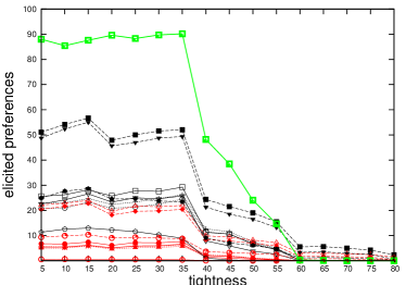
(c) d=50%, i=30%

Figure 4: Percentage of elicited preferences in incomplete fuzzy CSPs.

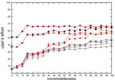
(a) d=50%, t=10%

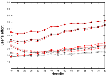
(b) t=10%, i=30%

Figure 5: Incomplete fuzzy CSPs: user’s effort

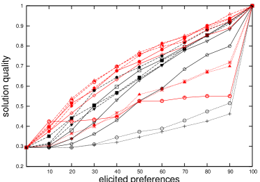
(a) solution quality

Figure 6: Incomplete fuzzy CSPs: solution quality.

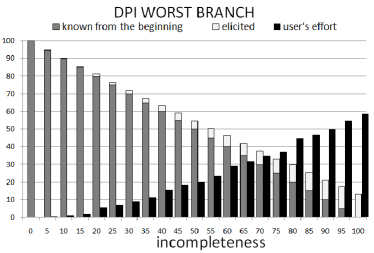
(a) d=50%, t=10%

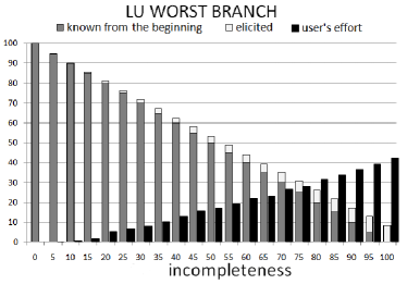
(b) d=50%, t=10%

Figure 7: Incomplete fuzzy CSPs: best algorithms.

5.2 Incomplete hard CSPs

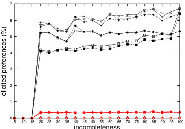
(a) d=50%, t=10%

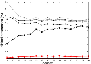
(b) t=10%, i=30%

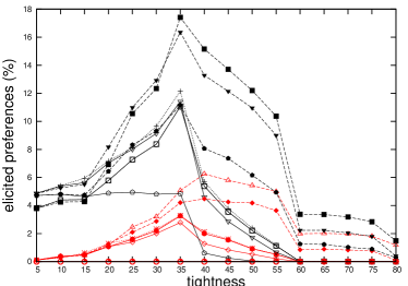
(c) d=50%, i=30%

Figure 8: Elicited preferences in incomplete CSPs.

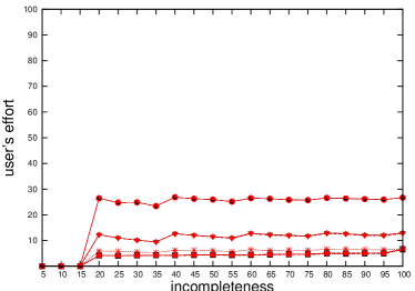
(a) d=50%, t=10%

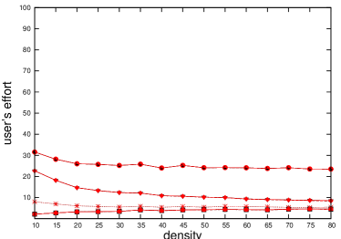
(b) t=10%, i=30%

Figure 9: Incomplete CSPs: user’s effort

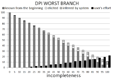
(a) d=50%, t=10%

Figure 10: Incomplete CSPs: best algorithm.

We also tested these algorithms on hard CSPs. In this case, preferences are only 0 and 1, and necessarily optimal solutions are complete assignments which are feasible in all completions. The problem generator is adapted accordingly. The parameter What now has a specific meaning: What=worst means asking if there is a 0 in the missing preferences. If there is no 0, we can infer that all the missing preferences are 1s.

Figure 8 shows the percentage of elicited preferences for hard CSPs in terms of amount of incompleteness, density, and tightness. Notice that the scale on the $y$ axis varies to include only the highest values. The best algorithms are those with What=worst, where the inference explained above about missing preferences can be performed. It is easy to see a phase transition at about 35% tightness, which is when problems pass from being solvable to having no solutions. However, the percentage of elicited preferences is below 20% for all algorithms even at the peak.

Figure 9 (a) shows the user’s effort in terms of amount of incompleteness and Figure 9 (b) shows the user’s effort in terms of density for the case of hard CSPs. Overall, the best algorithm is again DPI.WORST.BRANCH. Figure 10 gives the elicited preferences and user effort for this algorithm.

5.3 Incomplete temporal fuzzy CSPs

We also performed some experiments on fuzzy simple temporal problems [8]. These problems have constraints of the form $a\leq x-y\leq b$ modelling allowed time intervals for durations and distances of events, and fuzzy preferences associated to each element of an interval. We have generated classes of such problems following the approach in [8], adapted to consider incompleteness. While the class of problems generated in [8] is tractable, the presence of incompleteness makes them intractable in general. Figure 11 shows that in this specialized domain it is also possible to find a necessarily optimal solution by asking about 10% of the missing preferences, for example via algorithm DPI.WORST.BRANCH.

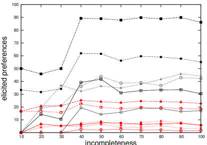
Figure 11: Percentage of elicited preferences in incomplete fuzzy temporal CSPs.

6 Future work

In the problems considered in this papers, we have no information about the missing preferences. We are currently considering settings in which each missing preference is associated to a range of possible values, that may be smaller than the whole range of preference values. For such problems, we intend to define several notions of optimality, among which necessarily and possibly optimal solutions are just two examples, and to develop specific elicitation strategies for each of them. We are also studying soft constraint problems when no preference is missing, but some of them are unstable, and have associated a range of possible alternative values.

To model fuzzy CSPs, we have not used traditional fuzzy set theory [3], but soft CSPs [1], since we intend to apply our work also to non-fuzzy CSPs. In fact, we plan to consider incomplete weighted constraint problems as well as different heuristics for choosing the next variable during the search. All algorithms with What=all are not tied to fuzzy CSPs and are reasonably efficient. Moreover, we intend to build solvers based on local search and variable elimination methods. Finally, we want to add elicitation costs and to use them also to guide the search, as done in [10] for hard CSPs.

References

- [1] S. Bistarelli, U. Montanari, and F. Rossi. Semiring-based constraint solving and optimization. JACM, 44(2):201–236, mar 1997.
- [2] R. Dechter and A. Dechter. Belief maintenance in dynamic constraint networks. In AAAI, pages 37–42, 1988.
- [3] D. Dubois and H. Prade. Fuzzy sets and Systems - Theory and Applications. Academic Press, 1980.
- [4] B. Faltings and S. Macho-Gonzalez. Open constraint satisfaction. In CP, volume 2470 of LNCS, pages 356–370. Springer, 2002.
- [5] B. Faltings and S. Macho-Gonzalez. Open constraint optimization. In CP, volume 2833 of LNCS, pages 303–317. Springer, 2003.
- [6] B. Faltings and S. Macho-Gonzalez. Open constraint programming. AI Journal, 161(1-2):181–208, 2005.
- [7] M. Gelain, M. S. Pini, F. Rossi, and K. B. Venable. Dealing with incomplete preferences in soft constraint problems. In Proc. CP’07, volume 4741 of LNCS, pages 286–300. Springer, 2007.
- [8] L. Khatib, P. Morris, R. Morris, F. Rossi, A. Sperduti, and K. Brent Venable. Solving and learning a tractable class of soft temporal problems: theoretical and experimental results. AI Communications, 20(3), 2007.
- [9] E. Lamma, P. Mello, M. Milano, R. Cucchiara, M. Gavanelli, and M. Piccardi. Constraint propagation and value acquisition: Why we should do it interactively. In IJCAI, pages 468–477, 1999.
- [10] N. Wilson, D. Grimes, and E. C. Freuder. A cost-based model and algorithms for interleaving solving and elicitation of csps. In Proc. CP’07, volume 4741 of LNCS, pages 666–680. Springer, 2007.