CP³-Origins: 2009-12, SU-4252-898
Perturbed S₃ neutrinos

Abstract

We study the effects of the perturbation which violates the permutation symmetry of three Majorana neutrinos but preserves the well known (23) interchange symmetry. This is done in the presence of an arbitrary Majorana phase $\psi$ which serves to insure the degeneracy of the three neutrinos at the unperturbed level.

I Introduction

In the present paper, a particular approach to understanding lepton mixing, proposed in jns and further studied in cw , will be examined in more detail. First, we briefly review the approach.

Of course, the standard model interaction term for $\beta$ decay or $\pi^{-}\rightarrow e^{-}\overline{\nu}_{e}$ includes the leptonic piece:

$${\cal L}=\frac{ig}{\sqrt{2}}W_{\mu}^{-}\overline{e}_{L}\gamma_{\mu}\nu_{e}+h.c,$$ (1)

The object $\nu_{e}$ is now known superK -minos to be a linear combination of neutrino mass eigenstates, ${\hat{\rho}}_{i}$:

$$\nu_{e}=\sum K_{ei}\widehat{\rho}_{i}$$ (2)

where, in a basis with the charged leptons diagonal, the full lepton mixing matrix is written as:

$$K=\left(\begin{array}[]{ccc}K_{e1}&K_{e2}&K_{e3}\\ K_{\mu 1}&K_{\mu 2}&K_{\mu 3}\\ K_{\tau 1}&K_{\tau 2}&K_{\tau 3}\\ \end{array}\right)$$ (3)

As has been discussed by many authors fx -hvvm the results of neutrino oscillation experiments are (neglecting possible phases to be discussed later) consistent with the “tribimaximal mixing” matrix:

$$K_{TBM}=\left(\begin{array}[]{ccc}\frac{-2}{\sqrt{6}}&\frac{1}{\sqrt{3}}&0\\ \frac{1}{\sqrt{6}}&\frac{1}{\sqrt{3}}&\frac{1}{\sqrt{2}}\\ \frac{1}{\sqrt{6}}&\frac{1}{\sqrt{3}}&\frac{-1}{\sqrt{2}}\\ \end{array}\right)\equiv R.$$ (4)

Many different approaches have been used to explain the form of $K$. A “natural”,and often investigated one uses the parallel three generation structure of the fundamental fermion families as a starting point. An underlying discrete symmetry $S_{3}$, the permutation group on three objects, is then assumed. w -mr The permutation matrices $S$ are,

$$S^{(1)} = \left[\begin{array}[]{ccc}1&0&0\\ 0&1&0\\ 0&0&1\end{array}\right],\hskip 21.68121ptS^{(12)}=\left[\begin{array}[]{ccc}0&1&0\\ 1&0&0\\ 0&0&1\end{array}\right],\hskip 21.68121ptS^{(13)}=\left[\begin{array}[]{ccc}0&0&1\\ 0&1&0\\ 1&0&0\end{array}\right],$$ (14)

$$S^{(23)} = \left[\begin{array}[]{ccc}1&0&0\\ 0&0&1\\ 0&1&0\end{array}\right],\hskip 21.68121ptS^{(123)}=\left[\begin{array}[]{ccc}0&0&1\\ 1&0&0\\ 0&1&0\end{array}\right],\hskip 21.68121ptS^{(132)}=\left[\begin{array}[]{ccc}0&1&0\\ 0&0&1\\ 1&0&0\end{array}\right],$$ (24)

This defining representation is not irreducible. The 3-dimensional space breaks up into irreducible 2-dimensonal and 1-dimensional spaces. One may note that the tribimaximal matrix, $K_{TBM}$ is an example of the transformation which relates the given basis to the irreducible one. This fact provides our motivation for further investigating the $S_{3}$ symmetry, even though many other interesting approaches exist. Of course, the symmetry requirement reads,

$$[S,M_{\nu}]=0,$$ (25)

where $S$ stands for any of the six matrices in Eq.(24) and $M_{\nu}$ is the neutrino mass matrix.

By explicitly evaluating the commutators one obtains the solution:

$$M_{\nu}=\alpha\left[\begin{array}[]{ccc}1&0&0\\ 0&1&0\\ 0&0&1\end{array}\right]+\beta\left[\begin{array}[]{ccc}1&1&1\\ 1&1&1\\ 1&1&1\\ \end{array}\right]\equiv\alpha{\bf 1}+\beta d.$$ (26)

$\alpha$ and $\beta$ are, in general, complex numbers for the case of Majorana neutrinos while $d$ is usually called the “democratic” matrix.

It is easy to verify that this $M_{\nu}$ may be brought to diagonal (but not necessarily real) form by the real orthogonal matrix, $R=K_{TBM}$ defined above:

$$R^{T}(\alpha{\bf 1}+{\beta}d)R=\left[\begin{array}[]{ccc}\alpha&0&0\\ 0&\alpha+3\beta&0\\ 0&0&\alpha\\ \end{array}\right].$$ (27)

$R$ may be written in terms of the eigenvectors of $M_{\nu}$ as:

$$R=\left[\begin{array}[]{ccc}\vec{r}_{1}&\vec{r}_{2}&\vec{r}_{3}\end{array}\right],$$ (28)

For example, $\vec{r}_{1}$ is the first column of the tribimaximal matrix, Eq.(4). Physically one can assign different masses to the mass eigenstate $\vec{r}_{2}$ in the 1-dimensional basis and to the (doubly degenerate) eigenstates $\vec{r}_{1}$ and $\vec{r}_{3}$ in the 2-dimensional basis. At first glance this sounds ideal since it is well known that the three neutrino masses are grouped into two almost degenerate ones (“solar neutrinos”) and one singlet, with different values. However, since we are demanding that R be taken as the tribimaximal form, the physical identification requires $\vec{r}_{1}$ and $\vec{r}_{2}$ to be the ”solar” neutrino eigenstates rather than the degenerate ones $\vec{r}_{1}$ and $\vec{r}_{3}$. This had been considered a serious objection to the present approach since often a scenario is pictured in which the mass eigenvalue for $\vec{r_{3}}$ is considerably larger than the roughly degenerate masses associated with $\vec{r_{1}}$ and $\vec{r_{2}}$. A way out was suggested in jns where it was noted that, for values of $m_{1}+m_{2}+m_{3}$ larger than around 0.3 eV, the neutrino spectrum would actually be approximately degenerate. This may be seen in detail by consulting the chart in Table 1 of jns wherein the neutrino masses are tabulated as a function of an assumed value of the third neutrino mass, $m_{3}$. Actually it is seen that there is also a region around $m_{3}\approx$ 0.04 eV and $m_{1}+m_{2}+m_{3}\approx 0.18eV$ where an assumed initial degeneracy may be reasonable. To make physical sense out of such a scenario, it was suggested that the neutrino mass matrix be written as,

$$M_{\nu}=M_{\nu}^{(0)}+M_{\nu}^{(1)}+M_{\nu}^{(2)},$$ (29)

where $M_{\nu}^{(0)}$ has the full $S_{3}$ invariance and has degenerate (at least approximately) eigenvalues. Furthermore, the smaller $M_{\nu}^{(1)}$ is invariant under a particular $S_{2}$ subgroup of $S_{3}$ and breaks the degeneracy. Finally, $M_{\nu}^{(2)}$ is invariant under a different $S_{2}$ subgroup of $S_{3}$ and is assumed to be smaller still. The strengths are summarized as:

$$M_{\nu}^{(0)}>M_{\nu}^{(1)}>M_{\nu}^{(2)}.$$ (30)

This is inspired by the pre-QCD flavor perturbation theory of the strong interaction which works quite well. In that case the initially unknown strong interaction Hamiltonian is expanded as

$$H=H^{(0)}+H^{(1)}+H^{(2)}.$$ (31)

Here $H^{(0)}$ is the dominant $SU(3)$ flavor invariant piece, $H^{(1)}$ is the smaller Gell-Mann Okubo perturbation gmo which transforms as the eighth component of a flavor octet representation and breaks the symmetry to SU(2) and $H^{(2)}$, which transforms as a different component of the octet representation and breaks the symmetry further to the hypercharge U(1), is smaller still.

There is a possible immediate objection to the assumption that the neutrino mass eigenvalues be degenerate in the initial S₃ invariant approximation; after all Eq.(27) shows that there are two different eigenvalues $\alpha$ and $\alpha+3\beta$. This was overcome by recognizing that these are both complex numbers and that they could both have the same magnitude but different directions. Having the same magnitude guarantees that all three physical masses will be the same. This introduces a physical phase $\psi$ corresponding to the angle between $\alpha$ and $\alpha+3\beta$.

In the strong interaction case, the initial SU(3) invariance was found to be reasonably well obeyed. It is thus natural to ask what predictions may exist in the initial $S_{3}$ invariant approximation in our neutrino model. It was found jns that the leptonic factor for neutrinoless double beta decay, $m_{ee}$ could be predicted in this limit to be,

$$|m_{ee}|=\frac{m}{3}\sqrt{5+4cos{\psi}},$$ (32)

where $m$ is the degenerate neutrino mass and $\psi$ is the Majorana type phase mentioned above. This led to the inequality

$$m>|m_{ee}|\geq m/3.$$ (33)

The next step in the program is to consider the effect of the perturbation $M_{\nu}^{(1)}$. Many authors mutau -Gutmutau have suggested that a $\mu$-$\tau$ symmetry ((23) symmetry in the present language) is associated with tribimaximal mixing in the neutrino sector. Thus it is a natural $S_{2}$ symmetry choice for $M_{\nu}^{(1)}$. Recently, Chen and Wolfenstein cw applied this type of perturbation to our present model with the additional assumption that the Majorana phase $\psi$ takes the value $\pi$. This corresponds to CP conservation. Their result for $|m_{ee}|$ is in agreement with the lower limit in Eq.(33). Here we will investigate the first perturbed case without assuming that special value of $\psi$.

Before going on to this we will present an amusing argument to show that the (23) perturbation is naturally associated with the tribimaximal form (modulo the majorana type phase $\psi$) rather than a tribimaximal form multiplied by a rotation in the two dimensional degenerate subspace (which is physically irrelevant at the $S_{3}$ invariant level). This is based on the fact that degenerate perturbation theory must be employed, which leads to a stability condition. Further we will show that other $S_{2}$ perturbations are mathematically consistent but do not lead to the desired tribimaximal form.

II Effects of different perturbations

In the present framework there are three different possible perturbations, each characterized by the $S_{2}$ subgroup which remains invariant. Let us first consider the favored perturbation which leaves invariant the S₂ subgroup, consisting of $S^{(1)}$ and $S^{(23)}$. Apart from a piece which may be reabsorbed in Eq.(26), such a perturbation has the form,

$$\Delta=\left(\begin{array}[]{ccc}0&0&0\\ 0&t&u\\ 0&u&t\\ \end{array}\right)$$ (34)

where $t$ and $u$ are parameters. It is convenient to adopt the language of ordinary quantum mechanics perturbation theory. We should then work in a basis like Eq.(27) where $M_{\nu}$ in Eq.(26) is diagonal. However, because of the double degeneracy between the eigenvectors $\vec{r}_{1}$ and $\vec{r}_{3}$ in Eq.(4), the matrix $R$ is not the unique one which diagonalizes $M_{\nu}$. We should really use the more general matrix $RX(\xi)$ where $X(\xi)$ is given by:

$$X(\xi)=\left(\begin{array}[]{ccc}cos\xi&0&-sin\xi\\ 0&1&0\\ sin\xi&0&\cos\xi\\ \end{array}\right).$$ (35)

In this basis $\Delta$ has the form:

$$X^{T}R^{T}\Delta RX=\left(\begin{array}[]{ccc}\frac{c^{2}(t+u)}{3}+s^{2}(t-u)&\frac{\sqrt{2}}{3}c(t+u)&\frac{2sc}{3}(t-2u)\\ \frac{\sqrt{2}}{3}c(t+u)&\frac{2}{3}(t+u)&-\frac{\sqrt{2}}{3}s(t+u)\\ \frac{2sc}{3}(t-2u)&-\frac{\sqrt{2}}{3}s(t+u)&\frac{s^{2}(t+u)}{3}+c^{2}(t-u)\\ \end{array}\right).$$ (36)

Here, $c=\cos\xi$ and $s=\sin\xi$. Note that, before adding a perturbation, the $S_{3}$ symmetry predicts the lepton mixing matrix to be $RX(\xi)$ rather than the desired tribimaximal form, $R$.

In perturbation theory, the first correction to the $m^{th}$ eigenvector involves the ratio $\frac{<n|H^{(1)}|m>}{E_{m}-E_{n}}$. For degenerate perturbation theory it is of course necessary that the numerator vanishes for those states with $E_{n}=E_{m}$. Here we simply require for the (13) matrix element:

$$(X(\xi)^{T}K_{TBM}^{T}\Delta K_{TBM}X(\xi))_{13}=0.$$ (37)

This yields in general, $sin(2\xi)=0$. The solution with $\xi=0$ is the desired tribimaximal form. The solution with $\xi=\pi$ just changes the signs of the first and third columns. However, the solutions with $\xi=\pi/2$ and $\xi=3\pi/2$ interchange the first and third columns, which does not agree with experiment. Thus, apart from a discrete ambiguity, the tribimaximal form is uniquely chosen when a smooth connection with the (23)-type perturbation is required. Of course, the smooth connection corresponds to choosing the correct initial states for the perturbation treatment.

It is easy to see that perturbations which leave the other two $S_{2}$ subgroups invariant, do not lead to mixing matrices of the desired tribimaximal form. The perturbation which commutes with $S^{(12)}$ is:

$$\Delta^{\prime}=\left(\begin{array}[]{ccc}t^{\prime}&u^{\prime}&0\\ u^{\prime}&t^{\prime}&0\\ 0&0&0\\ \end{array}\right).$$ (38)

Similarly, the perturbation which commutes with $S^{(13)}$ has the form:

$$\Delta^{\prime\prime}=\left(\begin{array}[]{ccc}t^{\prime\prime}&0&u^{\prime\prime}\\ 0&0&0\\ u^{\prime\prime}&0&t^{\prime\prime}\\ \end{array}\right).$$ (39)

The stability condition for obtaining the tribimaximal mixing for the $\Delta^{\prime}$ pertubation would require the matrix element $(K_{TBM}^{T}\Delta^{\prime}K_{TBM})_{13}$ to vanish; instead it takes the value $\frac{\sqrt{3}}{6}(t^{\prime}-2u^{\prime})$. Similarly, the stability condition for the $\Delta^{\prime\prime}$ pertubation does not work since the matrix element $(K_{TBM}^{T}\Delta^{\prime\prime}K_{TBM})_{13}$ takes the generally non-zero value $\frac{\sqrt{3}}{6}(-t^{\prime\prime}+2u^{\prime\prime})$.

While we have seen that the stability condition for (23) invariant perturbations enforces the experimentally plausible tribimaximal mixing, the underlying $S_{3}$ symmetry should allow characteristic stable mixing matrices to emerge for either the (12) invariant or (13) invariant perturbations. What are their forms? In the case of a (12) perturbation, the stability condition associated with degenerate perturbation theory reads:

$$(K^{T}\Delta^{\prime}K)_{13}=0.$$ (40)

Here the characteristic mixing matrix emerges as $K=K_{TBM}X(\xi)$ for a suitable value of $\xi$. The solution is easily seen to have the form:

$$K_{TBM}X(\frac{\pi}{6})=\left(\begin{array}[]{ccc}\frac{1}{\sqrt{3}}&\frac{1}{\sqrt{2}}&\frac{1}{\sqrt{6}}\\ \frac{1}{\sqrt{3}}&\frac{-1}{\sqrt{2}}&\frac{1}{\sqrt{6}}\\ \frac{1}{\sqrt{3}}&0&\frac{-2}{\sqrt{6}}\\ \end{array}\right).$$ (41)

In the case of a (13) invariant perturbation, the stability condition associated with degenerate perturbation theory reads:

$$(K^{T}\Delta^{\prime\prime}K)_{13}=0.$$ (42)

Here the characteristic stable mixing matrix turns out to be:

$$K_{TBM}X(\frac{\pi}{3})=\left(\begin{array}[]{ccc}\frac{-1}{\sqrt{6}}&\frac{1}{\sqrt{3}}&\frac{1}{\sqrt{2}}\\ \frac{2}{\sqrt{6}}&\frac{1}{\sqrt{3}}&0\\ \frac{-1}{\sqrt{6}}&\frac{1}{\sqrt{3}}&\frac{-1}{\sqrt{2}}\\ \end{array}\right).$$ (43)

The situation is summarized in Table 1. Mathematically, any of the three perturbations will result in a stable mixing matrix. However, only the (23) perturbation gives the experimentally allowed tribimaximal form. For example, we see that the zero value of $K_{13}$, in good present agreement with experiment, only holds for the $\Delta$ [(23)-type] perturbation.

Perturbation	Mixing matrix
$\Delta$	$K_{TBM}$
$\Delta^{\prime}$	$K_{TBM}X(\frac{\pi}{6})$
$\Delta^{\prime\prime}$	$K_{TBM}X(\frac{\pi}{3})$

Table 1: Characteristic, stable mixing matrices for each $S_{2}$ invariant perturbation.

III Zeroth order setup

In order to go further we adopt convenient conventions for the, in general, complex parameters $\alpha$ and $\beta$ defined in Eq.(26). The goal is to adjust a phase, $\psi$ in order that the zeroth order spectrum has three exactly degenerate neutrinos. As shown in Fig. 1, we take the 2-vector 3$\beta$ to be real positive. Then the 2-vector $\alpha$ lies in the third quadrant as:

$$\alpha=-i|\alpha|e^{-i\psi/2},$$ (44)

where the physical phase $\psi$ lies in the range:

$$o<\psi\leq\pi.$$ (45)

Finally $|\alpha|$ is related to $\beta$ by,

$$|\alpha|=\frac{3\beta}{2sin(\psi/2)}.$$ (46)

In the limiting case $\psi=\pi$, $\alpha$ takes the real value,

$$\alpha=-\frac{3\beta}{2}\hskip 56.9055pt(\psi=\pi).$$ (47)

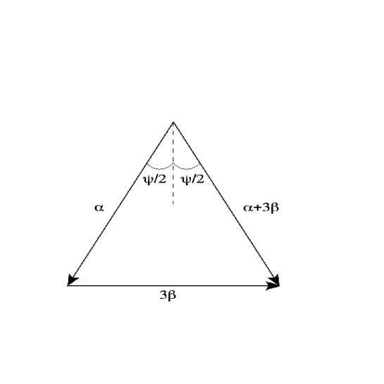
Figure 1: Isosceles triangle with angle $\psi$ between the equal length 2-vectors $\alpha$ and $\alpha+3\beta$.

IV Analysis of favored perturbation

For simplicity we will consider the parameters $t$ and $u$ in Eq.(34) to be real rather than complex. The entire neutrino mass matrix to first order is $M_{\nu}=\alpha{\bf 1}+\beta d+\Delta$. Since we are working in a basis where the zeroth order piece is diagonalized by the tribimaximal matrix, $R$, we must diagonalize the matrix:

$$R^{T}(\alpha{\bf 1}+\beta d+\Delta)R=$$

$$\alpha{\bf 1}+\left(\begin{array}[]{ccc}t+u&\frac{\sqrt{2}}{3}(t+u)&0\\ \frac{\sqrt{2}}{3}(t+u)&3\beta+\frac{2}{3}(t+u)&0\\ 0&0&t-u\\ \end{array}\right).$$ (51)

Diagonalizing the upper left 2 x 2 sub-matrix yields the three, in general, complex eigenvalues:

$$\alpha+\frac{3}{2}(\beta+T)(1-\sqrt{1-\frac{4\beta T}{3(\beta+T)^{2}}})\approx\alpha+T,$$

$$\alpha+\frac{3}{2}(\beta+T)(1+\sqrt{1-\frac{4\beta T}{3(\beta+T)^{2}}})\approx\alpha+3\beta+2T,$$

$$\alpha+t-u,$$ (52)

where we introduced the abbreviation, $T=(t+u)/3$. The indicated approximations to the exact eigenvalues correspond to working to first order in the parameters t and u. Remember that according to our original setup, t and u are supposed to be small compared to $|\alpha|$ and $\beta$. Since Fig. 1 shows that generally $|\alpha|>3\beta/2$, it is sufficient that $|t|$ and $|u|$ be small compared to $\beta$.

In this approximation the corresponding eigenvectors are the columns of,

$$R_{1}\approx\left(\begin{array}[]{ccc}1&\frac{\sqrt{2}}{9\beta}(t+u)&0\\ -\frac{\sqrt{2}}{9\beta}(t+u)&1&0\\ 0&0&1\\ \end{array}\right).$$ (53)

The entire diagonalization may be presented as,

$$K^{T}(\alpha{\bf 1}+\beta d+\Delta)K=\left(\begin{array}[]{ccc}m_{1}&0&0\\ 0&m_{2}&0\\ 0&0&m_{3}\\ \end{array}\right).$$ (54)

Here $m_{1}$, $m_{2}$ and $m_{3}$ are the three (positive) neutrino masses and

$$K=RR_{1}P$$ (55)

is the full neutrino mixing matrix (in a basis where the charged leptons are diagonal). The neutrino masses, to order $(t,u)/\beta$, are seen to be:

$$m_{1} \approx \frac{3\beta}{2}csc(\frac{\psi}{2})\left[1-\frac{2}{9\beta}(t+u)sin^{2}(\frac{\psi}{2})\right],$$

$$m_{2} \approx \frac{3\beta}{2}csc(\frac{\psi}{2})\left[1+\frac{4}{9\beta}(t+u)sin^{2}(\frac{\psi}{2})\right],$$

$$m_{3} \approx \frac{3\beta}{2}csc(\frac{\psi}{2})\left[1-\frac{6}{9\beta}(t-u)sin^{2}(\frac{\psi}{2})\right].$$ (56)

These mass parameters were made real, positive by the introduction of the phase matrix:

$$P=\left(\begin{array}[]{ccc}e^{-i\tau}&0&0\\ 0&e^{-i\sigma}&0\\ 0&0&e^{-i\rho}\\ \end{array}\right),$$ (57)

where,

$$\tau \approx \frac{\pi}{2}+\frac{1}{2}tan^{-1}[\frac{cot(\psi/2)}{1-\frac{2(t+u)}{9\beta}}]$$

$$\sigma \approx \pi-\frac{1}{2}tan^{-1}[\frac{cot(\psi/2)}{1+\frac{4(t+u)}{9\beta}}]$$

$$\rho \approx \frac{\pi}{2}+\frac{1}{2}tan^{-1}[\frac{cot(\psi/2)}{1-\frac{2(t-u)}{3\beta}}].$$ (58)

To compare with experiment, we have important information from neutrino oscillation experiments superK -minos . It is known that A

$$A \equiv m_{2}^{2}-m_{1}^{2}=(8\pm 0.3)\times 10^{-5}eV^{2},$$

$$B \equiv |m_{3}^{2}-m_{2}^{2}|=(2.5\pm 0.5)\times 10^{-3}eV^{2}.$$ (59)

Also, constraints on cosmological structure formation yield cosmobound a rough bound,

$$m_{1}+m_{2}+m_{3}<0.7eV.$$ (60)

The two allowed spectrum types are:

$$Type1:\hskip 28.45274ptm_{3}>m_{2}>m_{1},$$

$$Type2:\hskip 28.45274ptm_{2}>m_{1}>m_{3}.$$ (61)

.

Now, from Eq.(56) we see to leading order:

$$m_{2}^{2}-m_{1}^{2} = 3\beta(t+u),$$

$$m_{3}^{2}-m_{2}^{2} = \beta(-5t+u).$$ (62)

The quantities $\beta t$ and $\beta u$ may thus be obtained for a type 1 spectrum as:

$$\beta t=A/18-B/6\approx-4.13\times 10^{-4}eV^{2},$$

$$\beta u=5A/18+B/6\approx 4.39\times 10^{-4}eV^{2},$$ (63)

where the central experimental values were used. In the type 2 spectrum case, we should change $B\rightarrow-B$ in the above to find,

$$\beta t=A/18+B/6\approx 4.21\times 10^{-4}eV^{2},$$

$$\beta u=5A/18-B/6\approx-3.94\times 10^{-4}eV^{2}$$ (64)

Thus the, assumed real, $S_{3}$ violation parameters $\beta t$ and $\beta u$ are now known for each spectrum type. Information about the quantity $\beta$ may in principle be obtained from the perturbed lepton mixing matrix given in Eq. (55):

$$K\approx\left(\begin{array}[]{ccc}\frac{-2}{\sqrt{6}}-\frac{\sqrt{2}(t+u)}{9\beta\sqrt{3}}&\frac{1}{\sqrt{3}}-\frac{2(t+u)}{9\beta\sqrt{3}}&0\\ \frac{1}{\sqrt{6}}-\frac{\sqrt{2}(t+u)}{9\beta\sqrt{3}}&\frac{1}{\sqrt{3}}+\frac{(t+u)}{9\beta\sqrt{3}}&\frac{1}{\sqrt{2}}\\ \frac{1}{\sqrt{6}}-\frac{\sqrt{2}(t+u)}{9\beta\sqrt{3}}&\frac{1}{\sqrt{3}}+\frac{(t+u)}{9\beta\sqrt{3}}&\frac{-1}{\sqrt{2}}\\ \end{array}\right)P.$$ (65)

With a usual parameterization mns the matrix with zero (13) element takes the form,

$$K=\left(\begin{array}[]{ccc}c_{12}&s_{12}&0\\ -s_{12}c_{23}&c_{12}c_{23}&s_{23}\\ s_{12}s_{23}&-c_{12}s_{23}&c_{23}\\ \end{array}\right)P,$$ (66)

where $c_{12}$ is short for $cos\theta_{12}$ for example. This amounts to the predictions,

$$c_{12}=-\frac{2}{\sqrt{6}}-\frac{\sqrt{2}(\beta t+\beta u)}{9\sqrt{3}{\beta}^{2}},$$

$$c_{23}=-\frac{1}{\sqrt{2}},$$

$$s_{13}=0.$$ (67)

Notice that, when the perturbation is absent, this agrees with the tribimaximal form used here if both $\theta_{12}$ and $\theta_{23}$ lie in the second quadrant. The results of a recent study stv of neutrino oscillation experiments are:

$$(s_{23})^{2} = 0.50^{+0.07}_{-0.06},$$

$$(s_{12})^{2} = 0.304^{+0.022}_{-0.016}.$$ (68)

One immediately notices that the prediction, $(s_{23})^{2}$=1/2 is unchanged from its tribimaximal value by the perturbation and agrees with the new analysis. On the other hand the tribimaximal prediction, $(s_{12})^{2}$=1/3 is slightly changed from its tribimaximal value and actually lies slightly above the upper experimental error bar. This is probably not a serious disagreement but it might be instructive to try to fix it using the predicted perturbation in the present model:

$$(s_{12})^{2}=\frac{1}{3}-\frac{4}{27}\frac{\beta t+\beta u}{\beta^{2}}.$$ (69)

For either the type 1 or type 2 assumed spectrum, the perturbation is seen to be in the correct direction to lower the value of $s_{12})^{2}$, as desired. However, because of the large cancellation between $\beta t$ and $\beta u$, this effect is extremely small for a reasonable value of $\beta^{2}$; even with $\beta$ as small as 0.05 eV, $(s_{12})^{2}$ is only lowered to 0.332.

It is also interesting to discuss the absolute masses of the neutrinos rather than just the differences of their squares. Since the differences are known, let us focus on one of them, say $m_{3}$:

$$m_{3}\approx\frac{3\beta}{2}csc(\frac{\psi}{2})-\frac{\beta t-\beta u}{\beta}sin(\frac{\psi}{2}).$$ (70)

Notice that the first term on the right hand side is, using Eq.(46), simply the zeroth order degenerate mass, $|\alpha|$ while the second term represents the correction. Also note that (see Fig. 1) the point $\psi=0$ is not allowed. Considering $\psi$ as a parameter (related to the strength of neutrinoless double beta decay), this equation represents a quadratic formula giving $\beta$ in terms of the absolute mass $m_{3}$ for any assumed $\psi$. In Fig. 2, adopting the criterion that $|t|/\beta$ and $|u|/\beta$ be less than 1/5 for perturbative behavior, we display the perturbative region in the $m_{3}-\psi$ plane. In contrast to the case of $m_{3}$, $m_{1}$ and $m_{2}$ are seen to have small corrections since they of course depend on $\beta(t+u)$ rather than $\beta(t-u)$.

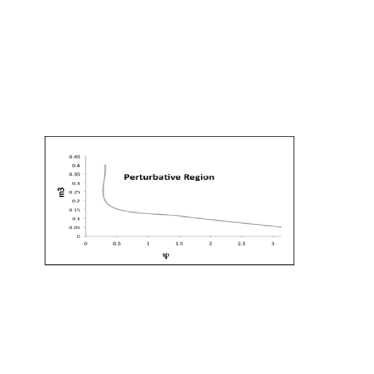
Figure 2: Sketch of perturbative region in the $m_{3}$-$\psi$ plane. It is about the same for both type 1 and type 2 neutrino spectra. Note that $\psi$ is measured in radians and $m_{3}$ is measured in eV.

V Neutrinoless double beta decay

The characteristic physical novelty of of a theory with Majorana type neutrinos is the prediction of a small, but non-zero, rate for the neutrinoless double beta decay of a nucleus: (A,Z) $\rightarrow$ (A,Z+2) + 2$e^{-}$. The appropriate leptonic factor describing the amplitude for this process is,

$$|m_{ee}|=|m_{1}(K_{11})^{2}+m_{2}(K_{12})^{2}+m_{3}(K_{13})^{2}|.$$ (71)

Substituting in the neutrino masses to order $(t,u)/\beta$ from Eq.(56 as well as Eq.(57) yields:

$$|m_{ee}|\approx\frac{3\beta}{2sin(\frac{\psi}{2})}|\frac{2}{3}+\frac{4(t+u)}{27\beta}cos^{2}(\frac{\psi}{2})+[\frac{1}{3}-\frac{4(t+u)}{27\beta}cos^{2}(\frac{\psi}{2})]e^{2i(\tau-\sigma})|.$$ (72)

The needed intermediate quantity $cos[2(\tau-\sigma)]$may be easily obtained from Eqs.(58) by construction of a suitable right triangles to be:

$$cos[2(\tau-\sigma)]\approx cos\psi-\frac{(t+u)sin\psi}{9\beta}.$$

We then find, correct to first order in $(t,u)/\beta$,

$$|m_{ee}|=\frac{\beta}{2sin(\psi/2)}\sqrt{5+4cos\psi},$$ (73)

which is just the zeroth order result. The experimental bound on $|m_{ee}|$ is given kka as,

$$|m_{ee}|<(0.35-1.30)eV,$$ (74)

which is small enough so that there is hope the possibility of a Majorana neutrino might be settled in the near future. Since the correction to $|m_{ee}|$ has been seen to be zero in this model we can take over the zeroth order inequality in Eq.(33). This means that the existence of the Majorana phase, $\psi$ can alter the amplitude for neutrinoless double beta decay by a factor of three for given (approximately degenerate) neutrino masses.

VI Summary and discussion

In some ways the problem of “flavor” in the Standard Model is reminiscent of that in Strong Interaction physics before the quark model. At that time it was realized that, as a precursor to detailed dynamics, group theory might give important clues.

Then the strong interactions were postulated to be SU(3) flavor invariant with a weaker piece having just the the SU(2) isospin (times hypercharge) invariance. In addition it was known that there was a still weaker isospin breaking (possibly QED) which by itself preserved a different SU(2) invariance (so-called U-spin).

Here, an analogy for neutrinos of the first two steps was studied in a perturbative framework. In jns and cw the possibility that the neutrinos are not strictly degnerate at the unperturbed level was contemplated. However in this paper we have examined a strictly degenerate first stage (setting to zero the parameters called respectively $\epsilon$ and $b$ in those two papers).

At the $S_{3}$ invariant level the neutrino mixing matrix is actually arbitrary up to a rotation in a 2-dimensional subspace. This problem can be settled (since degenerate perturbation theory is involved) by specifying the transformation property of the perturbation to be added. Although there is widespread agreement that the first perturbation should preserve the $S_{2}$ subgroup which interchanges the second and third neutrinos, we presented in section II, for completeness and interest, the mixing matrices for the other two possibilities also.

In sections III and IV we carried out the perturbation analysis for any choice of a Majorana-type phase, $\psi$ which plays an important role in this model. If $\psi$ is considered fixed there are three parameters in the model (In cw $\psi$ was considered fixed at the value $\pi$.) These three parameters can be taken as $\beta t$, $\beta u$ and $\beta$ defined above. The quantities $\beta t$ and $\beta u$ were found in terms of the neutrino squared mass differences for each choice of neutrino spectrum type, ie normal or inverted hierarchy. The value of $\beta$ depends on the presently unknown absolute value of any neutrino mass. The magnitudes of $\beta t$ and $\beta u$ are similar (though not exactly equal) but differ in sign. Thus the perturbation corrections which involve ($\beta t$ + $\beta u$) are very small. Clearly (see the first of Eqs.(62)) this is due to the small solar neutrino mass difference. This situation occurs for the correction to the mixing parameter $sin^{2}\theta_{12}$ in addition to $m_{1}$ and $m_{2}$, the masses of the first two neutrinos. The perturbation dependence on ($\beta t$ -$\beta u)$ is not suppressed however. This occurs for the mass, $m_{3}$ of the third neutrino. This result was used to make a sketch of the region in the $\psi$-$m_{3}$ plane for which the perturbation approach given seems numerically reasonable.

The explicit role of the Higgs sector, which is believed to be at the heart of the matter, was not discussed in the present paper. However, this as well as some further technical details were discussed in jns . Further treatment of this aspect is interesting for future work as is a detailed investigation of the weakest perturbation, the analog of the U-spin preserving perturbation in the strong interaction. This could be used to further study other consequences cw of possibly non-zero $\theta_{13}$.

VII acknowledgments

We are happy to thank Amir Fariborz, Salah Nasri and Francesco Sannino for helpful discussions and encouragment. The work of J. Schechter and M.N. Shahid was supported in part by the US DOE under Contract No. DE-FG-02-85ER 40231; they would also like to thank the CP³-Origins group at the University of Southern Denmark for their warm hospitality and partial support.

References

- (1) R. Jora, S. Nasri and J. Schechter, Int. J. Mod. Phys. A, 21, 5875 (2006).
- (2) C.-Y. Chen and L. Wolfenstein, Phys. Rev. D 77, 093009 (2008).
- (3) Super Kamiokande collaboration, S. Fukuda et al, Phys. Lett. B 539, 179 (2002), hep-ex/0205075.
- (4) KamLAND collaboration, K. Eguchi et al, Phys. Rev. Lett. 90, 021802 (2003).
- (5) SNO collaboration, Q. R. Ahmad et al,nucl-ex/ 0309004.
- (6) K2K collaboration, M. H. Ahn et al, Phys. Rev. Lett. 90, 041801 (2003).
- (7) GALLEX Collaboration, W. Hampel et al, Phys. Lett. B 447, 127 (1999).
- (8) SAGE Collaboration, J. N. Abdurashitov et al, Phys. Rev. C 60, 055801 (1999).
- (9) CHOOZ Collaboration, M. Apollonio et al, Eur. Phys. J. C 27, 331 (2003), hep-ex/0301017.
- (10) MINOS Collaboration, Phys. Rev. D 73, 072002 (2005), hep-ex/0512036.
- (11) H. Fritzsch and Z.-Z.Xing, Phys. Lett. B 440, 313 (1988), hep-ph/9808272.
- (12) P. F. Harrison, D. H. Perkins and W. G. Scott, Phys. Lett. B530,79 (2002), hep-ph/0202074.
- (13) Z.-Z.Xing, Phys. Lett. B 533, 85 (2002), hep-ph/020409.
- (14) X.G.He and A. Zee, Phys. Lett. B 560, 87 (2003), hep-ph/0204049.
- (15) P. F. Harrison and W. G. Scott, hep-ph/0302025.
- (16) C.I.Low and R.R.Volkas, Phys. Rev. D 68, 033007 (2003), hep-ph/0305243.
- (17) A.Zee, Phys. Rev. D 68, 093002 (2003), hep-ph/0307323.
- (18) J.D. Bjorken, P. F. Harrison and W. G. Scott, hep-ph/0511201.
- (19) R. N. Mohapatra, S. Nasri and H. B. Yu, arXiv:hep-ph/0605020.
- (20) S. F. King, Nucl. Phys. B 576, 85 (2000); S. F. King and N. N. Singh, Nucl. Phys. B 591, 3 (2000).
- (21) E. Ma, Phys. Rev. D 70 091301 (2004).
- (22) M. Hirsch, A. Velanova del Morel, J.W.F. Valle and E. Ma, Phys. Rev. D 72, (031901) (2005).
- (23) L. Wolfenstein, Phys. Rev. D 18, 958 (1978).
- (24) S. Pakvasa and H. Sugawara, Phys. Lett. B 73, 61 (1978); 82, 105 (1979); E. Derman and H.S.Tsao, Phys. Rev. D 20, 1207 (1979) and Y. Yamanaka, H. Sugawara and S. Pakvasa Phys. Rev. D 25, 1895 (1982).
- (25) S.-L. Chen, M. Frigerio and E. Ma, hep-ph/0404084.
- (26) M. Fukugita, M. Tanimoto and T. Yanagida, Phys. Rev. D 57, 4429 (1998), hep-ph/9709388.
- (27) E. Ma and G. Rajasekaran, Phys. Rev. D 64, 113012 (2001), hep-ph/0106291. —-
- (28) M. Gell-Mann, Phys. Rev. 125, 1067 (1962); S. Okubo, Prog. Theor. Phys. 27, 949 (1962); 28, 24 (1962).
- (29) T. Fukuyama and H. Nishiura, hep-ph/9702253; R. N. Mohapatra and S. Nussinov, Phys. Rev. D 60, 013002 (1999); E. Ma and M. Raidal, Phys. Rev. Lett. 87, 011802 (2001); C. S. Lam, hep-ph/0104116; T. Kitabayashi and M. Yasue, Phys.Rev. D67 015006 (2003); W. Grimus and L. Lavoura, hep-ph/0305046; 0309050; Y. Koide, Phys.Rev. D69, 093001 (2004);Y. H. Ahn, Sin Kyu Kang, C. S. Kim, Jake Lee, hep-ph/0602160; A. Ghosal, hep-ph/0304090; W. Grimus and L. Lavoura, Phys. Lett. B 572, 189 (2003); W. Grimus and L. Lavoura, J. Phys. G 30, 73 (2004).
- (30) W. Grimus, A. S.Joshipura, S. Kaneko, L. Lavoura, H. Sawanaka, M. Tanimoto, hep-ph/0408123; R. N. Mohapatra, JHEP, 0410, 027 (2004); A. de Gouvea, Phys.Rev. D69, 093007 (2004); R. N. Mohapatra and W. Rodejohann, Phys. Rev. D 72, 053001 (2005); T. Kitabayashi and M. Yasue, Phys. Lett,. B 621, 133 (2005); R. N. Mohapatra and S. Nasri, Phys. Rev. D 71, 033001 (2005);R. N. Mohapatra, S. Nasri and H. B. Yu, Phys. Lett. B 615, 231 (2005).
- (31) K. Matsuda and H. Nishiura, Phys. Rev. D 73, 013008 (2006); A. Joshipura, hep-ph/0512252; R. N. Mohapatra, S. Nasri and H. B. Yu, Phys. Lett. B 636, 114 (2006).
- (32) C. Amsler et al, Review of Particle Physics, Phys. Lett., B667:1 (2008).
- (33) D. N. Spergel et al, Astrophys. J. Suppl. 148: 175 (2003); S. Hannestad, JCAP 0305: 004 (2003).
- (34) See, for example, Eq. (10) of S.S. Masood, S. Nasri and J. Schechter, Phys. Rev. D 71, 093005 (2005). This reference also discusses a more symmetrical parameterization which may be convenient for treating neutrinoless double beta decay in general.
- (35) T. Schwetz, M. Tortola and J.W.F. Valle, arXiv:0808.2016.
- (36) H. V. Klapdor-Kleingrothaus et al, Eur. Phys. J. A 12, 147 (2001). See also the review, C. Aalseth et al, arXiv:hep-ph/0412300.