Induced magnetic moment in graphene with a nonmagnetic impurity

Abstract

We consider a two-dimensional crystalline monolayer of carbon atoms with a single non-magnetic impurity. Using the Weyl Hamiltonian to describe electronic energy spectrum near the Dirac points, we calculate the wave function and energy of impurity states, as well as the induced magnetic moment associated with polarization of the electron system. We present a phase diagram of the localized magnetic state as a function of the chemical potential $\mu$ and coupling constant $g_{c}$.

1 Introduction

Graphene has been attracting a lot of attention recently due to its unusual electronic structure and, correspondigly, due to its unique transport properties, which differ substantially from those of traditional metals and semiconductors [1, 2, 3]. The key characteristic features of graphene are the exact two-dimensionality of its crystal structure and massless relativistic energy spectrum near the Fermi surface. The Fermi surface transforms into isolated points in the clean limit of undoped graphene, and the electronic spectrum in the vicinity of these points can be described by the relativistic Dirac model. It is now commonly believed that these unusual properties of graphene make it an excellent candidate for various device applications in nanoelectronics and/or spintronics. [4].

Although there is great interest in magnetic properties of graphene, these are still not well understood. The main problem is that the usual doping with magnetic impurities like Mn or Fe can be ineffective because the magnetic atoms change dramatically the structure of electronic states due to bonding with carbon atoms. However, the possibility of doping with magnetic impurities, which can lead to ferromagnetism in graphene, has been discussed in several recent publications [5, 6, 7]. The main interest now is related to the possibility of magnetism induced by the presence of non-magnetic defects [8, 9, 10].

In this work we consider formation of a local magnetic moment in graphene, induced by a non-magnetic impurity. Assuming exchange coupling between the localized spin and electronic states we calculate magnetic polarization of the system and analyze conditions for the appearance of a local magnetic moment.

2 Model of graphene with a single impurity

The energy spectrum of graphene is described by the following tight-binding Hamiltonian [3],

$$\mathcal{H}_{tb}=\sum_{i}\varepsilon_{A}c_{Ai}^{{\dagger}}c_{Ai}+\sum_{n}\varepsilon_{B}c_{Bn}^{{\dagger}}c_{Bn}+t\sum_{<i,n>}(c_{Ai}^{{\dagger}}c_{Bn}+c_{Bn}^{{\dagger}}c_{Ai})$$ (1)

where the creation and annihilation operators correspond to electrons localized in atomic sites of two nonequivalent sublattices $A$ and $B$, with the hopping between the nearest neighbors of different sublattices described by the parameter $t$. The indices $i$ and $n$ refer to sites in the sublattices $A$ and $B$, respectively. The onsite energy in graphene is the same for both sublattices, $\varepsilon_{A}=\varepsilon_{B}$.

By transforming Hamiltonian (1) (with $\varepsilon_{A}=\varepsilon_{B}$) to the momentum representation, one reproduces the energy spectrum of graphene, which has two nonequivalent Dirac points in the $k$ space, with a linear energy spectrum near these points. The Dirac points are known to be the most interesting features of the electronic structure, because the Fermi level of graphene is usually located at these points or in their close vicinity.

In our calculations we restrict ourselves to the energy spectrum near the Dirac points. The corresponding Hamiltonian is known in quantum field theory as the 2D Weyl Hamiltonian of massless relativistic particles,

$$\mathcal{H}_{0}=\left(\begin{array}[]{cc}0&v\hbar\,(k_{x}-ik_{y})\\ v\hbar\,(k_{x}+ik_{y})&0\end{array}\right)=v\hbar\mbox{\boldmath$\tau$}\cdot{\bf k},$$ (4)

where $v$ is the velocity of electrons, which in graphene is $v\simeq 10^{6}\,m/s$, $\tau$ are the Pauli matrices acting in the sublattice space (matrices of pseudospin), and we put the energy onset in the Dirac points, $\varepsilon_{A}=\varepsilon_{B}=0$.

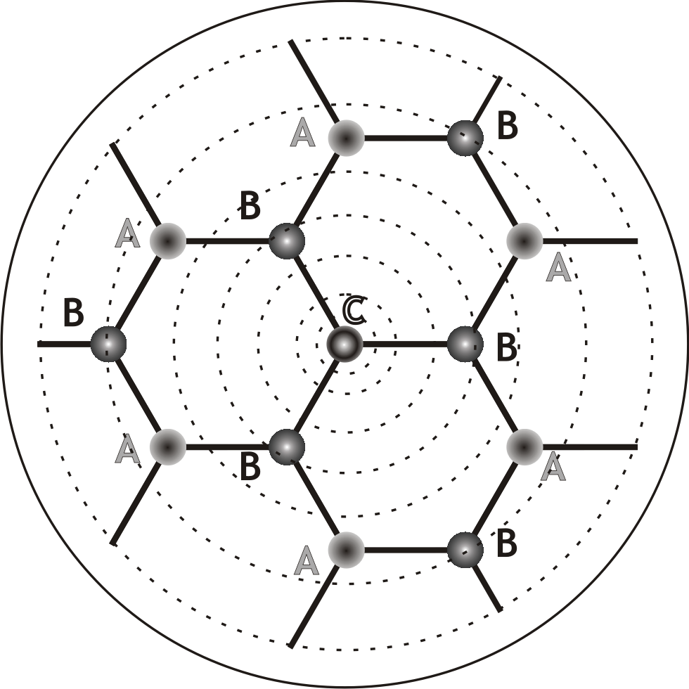
Figure 1: Schematic view of an impurity $C$, which substitutes a carbon atom in the sublattice $A$ of graphene.

In the following we assume that one carbon atom in the sublattice $A$ is replaced by an impurity atom $C$ (located at $\mathbf{r}=\mathbf{0}$), as shown schematically in Fig. 1. This replacement can be formally included in the Hamiltonian (1) as a term with onsite energy $\varepsilon_{C}$ at the site $i=0$, so that the perturbation is $V_{0}=(\varepsilon_{C}-\varepsilon_{A})c_{A0}^{{\dagger}}c_{A0}$. After reducing to the Weyl Hamiltonian, the corresponding perturbation term in the polar coordinates ($\rho,\phi$)

$$\mathcal{H}_{int}=\left(\begin{array}[]{cc}V_{0}\,\delta(\rho)&0\\ 0&0\end{array}\right).$$ (5)

3 Localized electronic states

Our task now is to find impurity states described by the Hamiltonian $\mathcal{H}=\mathcal{H}_{0}+\mathcal{H}_{int}$, with $\mathcal{H}_{0}$ and $\mathcal{H}_{int}$ defined by Eqs. (2) and (3), respectively. The corresponding Schrödinger equation, $(\mathcal{H}-\varepsilon)\Psi(\rho,\varphi)=0$, gives us the energy and eigenfunction of the localized electronic states.

Solving the Schrödinger equation for $\rho\neq 0$ we find a general solution in the form of a superposition of the Bessel functions $J_{m}(\xi)$ and $Y_{m}(\xi)$, where $\xi=\rho\varepsilon/\hbar v)$ and $m$ is the magnetic quantum number. It turns out that only the following pseudospinor form of the solution gives us the localized states near the Dirac point:

$$\Psi_{m}(\varrho,\varphi)=N\left(\begin{array}[]{l}e^{im\varphi}\,Y_{m}(\xi)\\ \displaystyle{i\,e^{i(m+1)\varphi}}\,Y_{m+1}(\xi)\end{array}\right),$$ (8)

where $N$ is the normalization factor.

Energy of the localized states can be found by integrating the Schrödinger equation with the wavefunction (4) over a small area near the point $\rho=0$. Within the lattice model, this corresponds to integration over $\rho<a_{0}$, where $a_{0}$ is the lattice parameter. This way we account for the boundary condition at $\rho=0$ with the $\delta$-like perturbation localized at this point. The ground state corresponds to the choice $m=0$ or $m=-1$. Both states give us the same energy of the localized state,

$$\varepsilon_{0}=\frac{2\pi\,\hbar^{2}v^{2}}{V_{0}\ln\left(a_{0}|\varepsilon_{0}|/\hbar v\right)}\simeq\frac{2\pi\,\hbar^{2}v^{2}}{V_{0}\ln\left(2\pi a_{0}\hbar v/|V_{0}|\right)}.$$ (9)

As we see from the solution (5), the energy of the localized state $\varepsilon_{0}\to 0$ as the perturbation $|V_{0}|$ increases. For the parameters typical of graphene, the sign of  logarithm in (5) is negative, and therefore the sign of the energy state $\varepsilon_{0}$ is opposite to that of perturbation potential. In other words, the attractive (negative) potential, $V_{0}<0$, gives us a state with the energy $\varepsilon_{0}>0$ and vice versa. This is just the opposite behavior as compared to the impurity state in traditional semiconductors – if we assume that graphene is similar to the gapless semiconductors. An important point is the above mentioned degeneracy of localized states, which is related to the pseudospinor wave function in graphene.

We have also checked the result (5) for the energy of impurity state by calculating the exact $T$-matrix of scattering from the impurity described by the matrix perturbation (3). Both calculation methods give exactly the same results.

4 Induced magnetic moment

The impurity state in graphene is occupied by an electron when the Fermi level is above the impurity level (5). Hence, in our consideration we assume that the location of the Fermi level is an independent parameter which is not related with the single impurity state under consideration. In reality, this assumption is well justified because position of the Fermi level in graphene is usually related with various defects or simply can be controlled by a gate voltage.

The single electron localized at the impurity has the magnetic moment $\mu_{B}$. In the following consideration we assume that the Coulomb interaction does not allow for two or more electrons to occupy the same impurity state, which means that the Hubbard energy is sufficiently large.

Magnetic moment of the localized electron polarizes the electron system, inducing magnetic moment whose magnitude depends on the magnetic polarizability of the electron gas in graphene. Assuming exchange coupling of electrons in graphene with the localized electrons we calculate the induced magnetic moment. The Hamiltonian of such an exchange interaction is

$$H^{m}_{int}=\frac{1}{2}\,g_{c}\mu_{z}(\mathbf{r})\sigma_{z},$$ (10)

where $g_{c}$ is the coupling constant, $\mu_{z}({\bf r})$ is the spatial distribution of magnetization associated with the wavefunction profile of the localized electron in Eq. (4),

$$\mu_{z}({\bf r})=g\mu_{B}|\Psi({\bf r})|^{2},$$ (11)

and $\sigma_{z}$ is the Pauli matrix for electron spin. We take the quantization axis along the spin orientation of the localized electron.

The induced magnetic moment ${\bf M}({\bf r})$ of electrons in graphene can be calculated using the quantum field theoretical method, used for calculation of magnetic polarizability [11]. Accordingly, one can present it as a loop Feynman diagram, which gives

$$M_{z}({\bf r})=ig_{c}g\mu_{B}\,{\rm Tr}\int d^{2}\mathbf{r^{\prime}}\,\int\frac{d\varepsilon}{2\pi}\,\sigma_{z}\,G_{0}\left(\varepsilon,\mathbf{r}-\mathbf{r^{\prime}}\right)\sigma_{z}G_{0}\left(\varepsilon,{\bf r^{\prime}}-{\bf r}\right)\,\mu_{z}({\bf r^{\prime}}),$$ (12)

where $G_{0}(\varepsilon,{\bf r})$ is the Green function of electrons in graphene in the energy-coordinate representation. The calculation of the Green function using the Hamiltonian (2) gives

$$G_{0}(\varepsilon,\pm\mathbf{r})=-\frac{i\varepsilon}{4\hbar^{2}v^{2}}H_{0}^{(1)}\left(\frac{r\varepsilon}{\hbar v}\right)\pm\mbox{\boldmath$\tau$}\cdot{\bf r}\frac{\varepsilon}{4r\hbar^{2}v^{2}}H_{1}^{(1)}\left(\frac{r\varepsilon}{\hbar v}\right),$$ (13)

where $H^{(1)}_{0,1}$ are the Hankel functions [12]. Using Eqs. (7)-(9) we find

$$M_{z}(\mathbf{r})=-\frac{g_{c}g\mu_{B}\zeta}{4\pi\hbar v}\int d^{2}\mathbf{r^{\prime}}\;\frac{\mu_{z}(\mathbf{r^{\prime}})}{|{\bf r}-{\bf r}^{\prime}|^{3}},$$ (14)

where

$$\zeta=\int\limits^{\infty}_{0}d\xi\,\xi^{2}\left[K^{2}_{0}(\xi)+K^{2}_{1}(\xi)\right],$$ (15)

and

$$K_{m}(\xi)=\frac{i^{m+1}\pi}{2}H_{m}^{(1)}(i\xi)$$ (16)

is the the modified Bessel function [12].

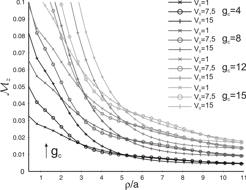
Figure 2: The density of induced magnetic moment as a function of the distance $\rho$ for different coupling parameters.

Using Eqs. (10)-(12) one can write the induced magnetic moment in the following form:

$$M_{z}(\rho)=\frac{g_{c}g^{2}\mu_{B}^{2}\pi}{8\hbar v}\int_{0}^{\infty}\frac{\rho^{\prime}|\psi(\rho^{\prime})|^{2}\mathcal{E}\left(\varsigma\right)}{(\rho+\rho^{\prime})(\rho-\rho^{\prime})^{2}}\;d\rho^{\prime}$$ (17)

where $\mathcal{E}\left(\varsigma\right)$ is the elliptic integral of the second kind and $\varsigma=2\sqrt{\rho\rho^{\prime}}/{(\rho+\rho^{\prime})}$. This expression was used for the numerical calculations, and the results are presented in Fig. 2.

We have also calculated the total induced magnetic moment

$$M_{0}(V_{0},g_{c})=2\pi\int\limits_{0}^{\infty}M_{z}(\rho)\,\rho d\rho$$ (18)

The dependence of $M_{0}$ on the strength of impurity potential $|V_{0}|$ is found to be rather weak, whereas the main factor which may enhance $M_{0}$ is the magnitude of the coupling parameter $g_{c}$.

5 Magnetic coupling of the localized spin with induced magnetic moment

The magnetic interaction of the localized spin with induced magnetic density $M_{z}(\rho)$ leads to the renormalization of the impurity energy level [13]. This interaction can be written as

$$E_{int}=-2\pi g_{c}\int\limits_{0}^{\infty}M_{z}(\mathbf{\varrho})|\Psi(\varrho)|^{2}\,\rho\,d\rho.$$ (19)

We have calculated numerically the interaction (15) and found the corresponding shift of the energy level. Our results are presented in Fig. 3.

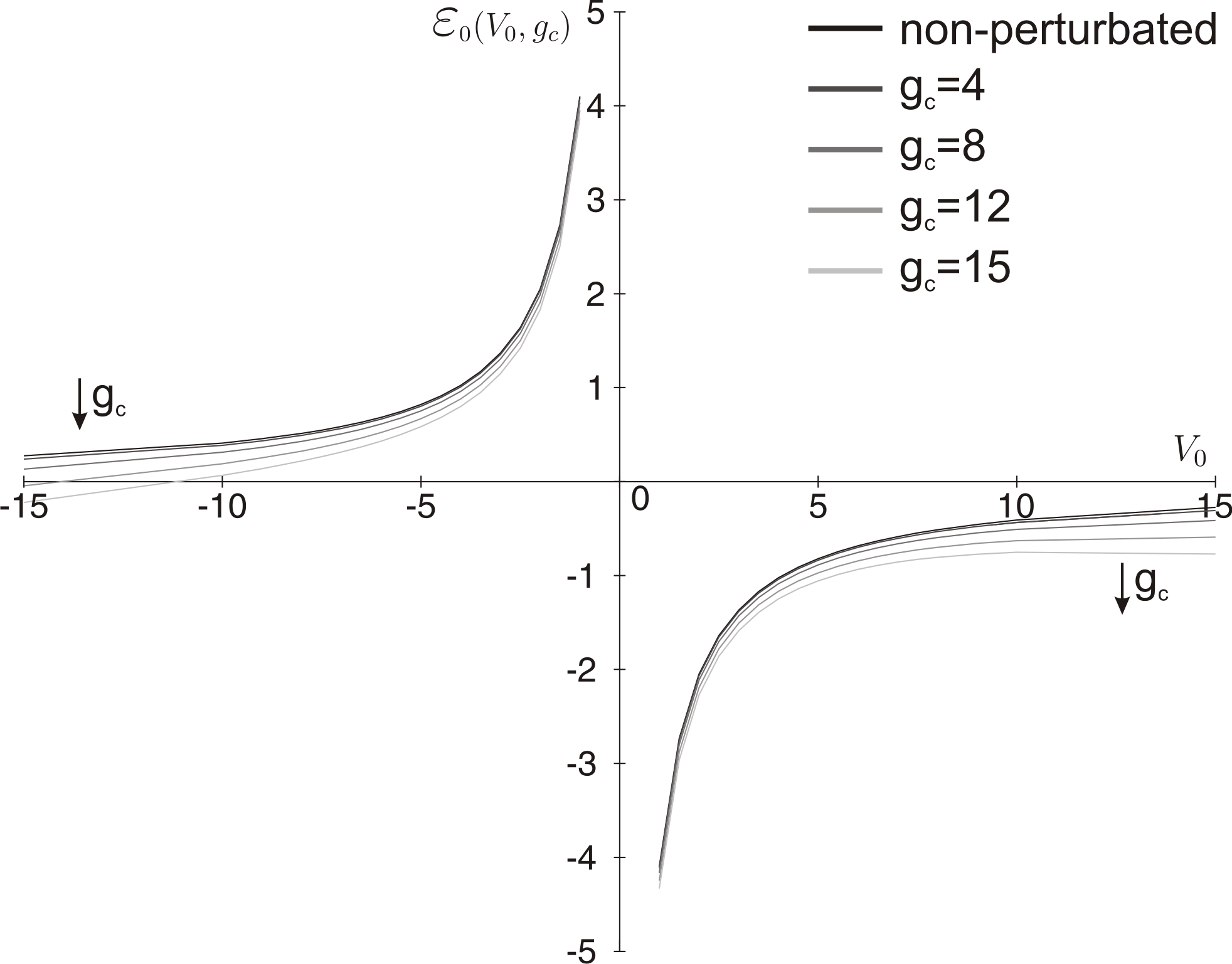
Figure 3: Energy level of the localized electron interacting with the induced magnetic moment for different values of the coupling constant $g_{c}$. The energy in the units of hopping t.

6 Phase diagram

The obtained results can be presented in the form of a phase diagram, Fig. 4, which shows the regions of the parameters $V_{0}$ and $\mu$, for which the impurity level is occupied with electron inducing the local magnetization around impurity. It should be pointed out that the level can be occupied even if the nonrenormalized position of the level is above the Fermi energy [13]. This result is related to the effect of onsite magnetic correlations.

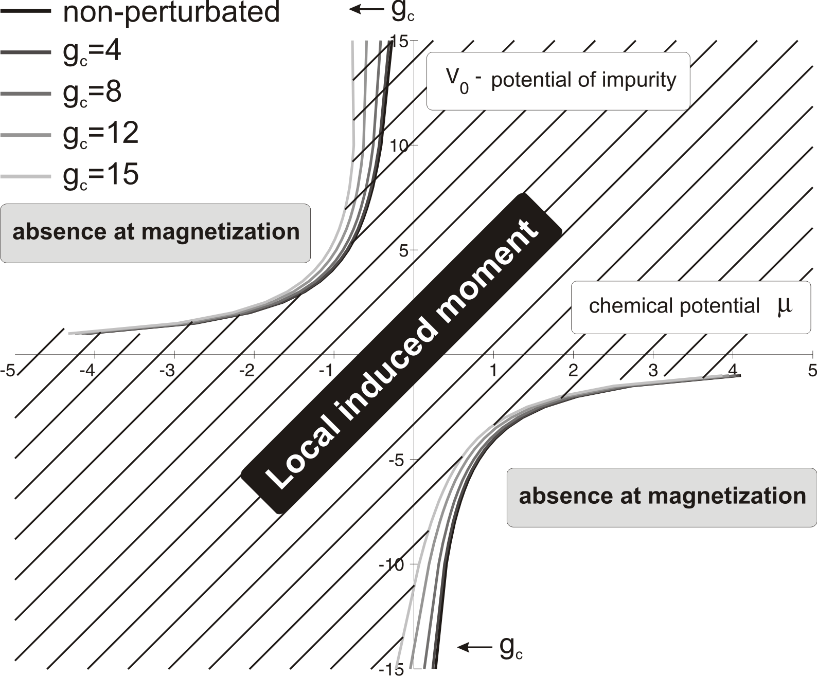
Figure 4: The phase diagram with the dashed area corresponding to the local magnetic moment induced by a nonmagnetic impurity.

7 Conclusion

The results of our calculations show that the nonmagnetic impurity can create an induced localized magnetic state due to the local electronic correlations. It should be emphasized that this effect is not related to free electrons because the density of free electrons in graphene can be vanishingly small. However, the magnetic polarizability of the electron system is large and long-range even without free electrons, which is the main reason for the local ferromagnetism.

This work is supported by the Polish Ministry of Science and Higher Education as a research project in years 2007 – 2010 and by FCT Grant PTDC/FIS/70843/2006 in Portugal.

References

References

- [1] Novoselov K S, Geim A K, Morozov S V, Jiang D, Katsnelson M I, Grigorieva I V, Dubonos S V, and Firsov A A 2005 Nature 438 197
- [2] Geim A K and Novoselov K S 2007 Nature Materials 6 183
- [3] Castro Neto A H, Guinea A, Peres N M R, Novoselov K S and Geim A K 2009 Rev Mod Phys 81 109
- [4] Avouris P, Chen Z and Perebeinos V 2007 Nature Nanotechnology 2 605
- [5] Vozmediano M A H, López-Sancho M P, Stauber T and Guinea F 2005 Phys Rev B 72 155121
- [6] Peres N M P, Guinea F and Castro Neto A H 2005 Phys Rev B 72 174406
- [7] Dugaev V K, Litvinov V I and Barnaś J 2006 Phys Rev B 74 224438
- [8] Yazyev O V and Helm L 2007 Phys Rev B 75 125408
- [9] Uchoa B, Kotov V N, Peres N M R and Castro Neto A H 2008 Phys Rev Lett 101 026805
- [10] Yazyev O V 2008 Phys Rev Lett 101 037203
- [11] Abrikosov A A Gorkov L P and Dzyaloshinski I E 1963 Methods of Quantum Field Theory in Statistical Physics (New York: Dover)
- [12] Abramowitz M and Stegun I A 1965 Handbook of Mathematical Functions (New York: Dover)
- [13] Abrikosov A A 1973 Sov Phys JETP 65 814