Amplitude Noise Supression in Cavity-Driven Oscillations of a Mechanical Resonator

Abstract

We analyze the amplitude and phase noise of limit-cycle oscillations in a mechanical resonator coupled parametrically to an optical cavity driven above its resonant frequency. At a given temperature the limit-cycle oscillations have lower amplitude noise than states of the same average amplitude excited by a pure harmonic drive; for sufficiently low thermal noise a sub-Poissonian resonator state can be produced. We also calculate the linewidth narrowing that occurs in the limit-cycle states and show that while the minimum is set by direct phase diffusion, diffusion due to the optical spring effect can dominate if the cavity is not driven exactly at a side-band resonance.

Recently there has been considerable progress towards the goal of observing signatures of quantum behavior in the collective vibrations of mechanical resonators AS . Evidence of quantum behavior is expected to be found in the production of non-classical states of mechanical motion such as squeezed states or superpositions of spatially separated states mpb ; AS . Quantum effects should also be evident in the non-linear dynamics of mechanical resonators ron , as well as in the fundamental limits on the sensitivity with which mechanical motion can be monitored limits . However, because mechanical resonators typically have resonant frequencies in the radio-frequency range or below, thermal fluctuations would naturally tend to mask the quantum features and hence significant efforts have been devoted to developing ways of cooling a mechanical resonator down to its ground state AS ; omechrev .

The radiation pressure force which arises when a mechanical resonator is coupled parametrically to a driven optical cavity omechrev provides a very effective way of suppressing thermal fluctuations in mechanical resonators. When the cavity is driven below resonance, quanta are absorbed from the mechanical resonator by the cavity. The low level of photon noise in the cavity means that, provided the relaxation rate of the cavity is much less than the mechanical frequency (the good cavity limit), the mechanical resonator can in principle be cooled almost all the way to its ground state MCCG . However, in practice the cooling effect of the cavity competes with the resonator’s thermal environment and recent experiments recent have combined the driven cavity with cryogenic cooling to achieve lower occupation numbers.

If the cavity is instead driven above resonance then energy is absorbed by the mechanical resonator leading to states of self-sustaining oscillation LC ; MHG . Increasing the power of the cavity drive leads eventually to a region of multistability marked by a sequence of dynamical transitions between limit-cycle states of different sizes LC ; MHG . Little attention has so far been devoted to studying the quantum aspects of the limit-cycle dynamics, although recent numerical calculations began to explore the behavior in this regime LKM . However, similar laser-like states have been studied in mechanical oscillators coupled to a range of finite-level systems CB ; HRA ; vpl .

In this Letter, we present an analytic calculation of the amplitude noise of a cavity-driven mechanical resonator within a limit-cycle. Our principal finding is that the amplitude noise in a limit-cycle can be very low: for very low thermal noise the resonator can be driven into a sub-Poissonian state by the cavity. More generally, at a given temperature the amplitude noise in a limit-cycle state can be substantially lower than in an equivalent one produced by a perfect harmonic drive. We also explore the behavior of the resonator linewidth in the limit-cycle state, generalizing a previous calculation vah .

The parametrically coupled driven cavity and mechanical resonator system is described by MCCG ; MHG ,

$$H=-\hbar[\Delta+\frac{g}{2}(b+b^{\dagger})]a^{\dagger}a+\hbar\omega_{m}b^{\dagger}b+\hbar\Omega(a+a^{\dagger}),$$ (1)

where $g$ is the coupling strength, $a$($b$) is a cavity (resonator) lowering operator, $\omega_{m}$ is the mechanical frequency and $\Omega$ parameterizes the strength of the laser drive. The cavity is driven at a frequency $\omega_{d}$ detuned from the cavity frequency, $\omega_{c}$ ($\gg\omega_{m}$), by $\Delta=\omega_{d}-\omega_{c}$. The evolution of the system is described by the master equation LKM ,

$$\dot{\rho}=-\frac{i}{\hbar}[H,\rho]+\mathcal{L}_{m}\rho+\mathcal{L}_{c}\rho,$$ (2)

where the coupling of the mechanical resonator to its thermalized surroundings at temperature $T$ is described by,

$$\mathcal{L}_{m}\rho = -\frac{\gamma_{m}}{2}(\overline{n}+1)\left(b^{\dagger}b\rho+\rho b^{\dagger}b-2b\rho b^{\dagger}\right)$$

$$-\frac{\gamma_{m}}{2}\overline{n}\left(bb^{\dagger}\rho+\rho bb^{\dagger}-2b^{\dagger}\rho b\right),$$

with $\gamma_{m}$ the mechanical damping rate and $\bar{n}=[{\rm exp}(\hbar\omega_{m}/k_{\rm B}T)-1]^{-1}$. The cavity dissipation is described by, $\mathcal{L}_{c}\rho=-\gamma_{c}(a^{\dagger}a\rho+\rho a^{\dagger}a-2a\rho a^{\dagger})/2$ with $\gamma_{c}$ the decay rate and we assume $\hbar\omega_{c}\gg k_{\rm B}T$ so that we can neglect thermal fluctuations.

We proceed by carrying out a Wigner transformation of the master equation, which introduces the complex variables $\alpha$ and $\beta$ for the phase space of the cavity and resonator respectively WM . Neglecting third-order derivative terms (truncated Wigner function approximation) in the resulting equation of motion for the Wigner function leads to a standard Fokker-Planck equation from which we obtain the coupled Langevin equations,

$$\dot{\alpha} = i[\Delta+\frac{g}{2}(\beta+\beta^{*})]\alpha-i\Omega-\frac{\gamma_{c}}{2}\alpha+\eta_{\alpha}$$ (3)

$$\dot{\beta} = i\frac{g}{2}\left(\alpha^{*}\alpha-\frac{1}{2}\right)-i\omega_{m}\beta-\frac{\gamma_{m}}{2}\beta+\eta_{\beta}.$$ (4)

The stochastic force terms WM $\eta_{\alpha},\eta_{\beta}$ have zero means and non-zero second order moments ${\left\langle\eta_{\alpha^{*}}(t)\eta_{\alpha}(t^{\prime})\right\rangle}=\delta(t-t^{\prime})\gamma_{c}/2$ and ${\left\langle\eta_{\beta^{*}}(t)\eta_{\beta}(t^{\prime})\right\rangle}=\delta(t-t^{\prime})\gamma_{m}(\bar{n}+\frac{1}{2})$. The truncated Wigner function approximation is expected to describe small linear fluctuations WM and hence should provide a good description for the limit-cycle states.

We follow the approach used by Marquardt et al. MHG to solve the corresponding classical dynamics and extend this to include the noise. We make the realistic assumption that the total resonator damping is much lower than the cavity decay rate so that the amplitude and phase of the resonator change only very slowly on the time-scale of the cavity dynamics. The problem is now split into two parts. First, we solve for $\alpha$ using the ansatz $\beta(t)=\beta_{c}+B{\rm e}^{-i\phi}{\rm e}^{-i\omega_{m}t}$. The resulting solution is split into average and fluctuating parts, $\alpha(t)=\langle\alpha(t)\rangle+\delta\alpha$ (where the average corresponds to the solution obtained when the stochastic force term is dropped) and then assuming weak fluctuations we approximate $\alpha\alpha^{*}\simeq\langle\alpha\alpha^{*}\rangle+\delta\alpha^{*}\langle\alpha\rangle+\delta\alpha\langle\alpha^{*}\rangle$ to obtain an effective equation of motion for $\tilde{\beta}(t)=\beta(t)-\beta_{c}$.

Solving for the cavity dynamics and taking the Fourier transform, we obtain

$$\langle\alpha^{\prime}(\omega)\rangle=\sum_{n}\alpha_{n}\delta(\omega-\omega_{m}n)=\frac{-i\Omega\sum_{n}J_{-n}(z){\rm e}^{i\phi n}\delta(\omega-\omega_{m}n)}{\gamma_{c}/2+i(\omega-\tilde{\Delta})}$$

and $\delta\alpha^{\prime}(\omega)={\eta^{\prime}_{\alpha}}/[{\gamma_{c}/2+i(\omega-\tilde{\Delta})}]$, where $z=gB/\omega_{m}$, $J_{n}(z)$ is a Bessel function of the first kind, $\tilde{\Delta}=\Delta+g{\rm Re}[\beta_{c}]$ and the primes denote e.g. $\eta^{\prime}_{\alpha}(t)=\eta_{\alpha}(t){\rm e}^{-iz\sin(\phi+\omega t)}$. Keeping only the fundamental oscillating component of $\langle\alpha\rangle\langle\alpha^{*}\rangle$, we obtain

$$\dot{\tilde{\beta}}=-\frac{(\gamma_{BA}+\gamma_{m})}{2}\tilde{\beta}-i(\omega_{m}+\delta\omega_{m})\tilde{\beta}+\eta_{\beta}+\frac{ig}{2}(\langle\alpha^{*}\rangle\delta\alpha+\langle\alpha\rangle\delta\alpha^{*}),$$ (5)

where the effective damping and frequency shift of the resonator due to the cavity are given by MHG ,

$$\frac{\gamma_{BA}}{2}+i\delta\omega_{m} = \frac{-ig\Omega^{2}}{2B}\sum\limits_{n}\frac{J_{n}(z)J_{n+1}(z)}{h_{n}h_{n+1}^{*}},$$ (6)

with $h_{n}=\frac{\gamma_{c}}{2}+i(\tilde{\Delta}+n\omega_{m})$. The center of the mechanical oscillations is given by,

$$\beta_{c} = \frac{ig}{2}\frac{\sum\limits_{n}|\alpha_{n}|^{2}}{i\omega_{m}+\frac{\gamma_{m}}{2}},$$ (7)

which, although non-linear, is well approximated by its linear form for weak $g$.

We focus for now on the fluctuations in the amplitude of the resonator motion. The equation of motion for the amplitude can be written as,

$$\dot{B}=-\frac{\gamma_{T}}{2}B+\eta_{T}^{-},$$ (8)

where $\gamma_{T}=\gamma_{m}+\gamma_{BA}$ and $\eta_{T}^{\mp}=\frac{1}{2}(\eta_{\beta}{\rm e}^{i(\phi+\omega_{m}t)}\pm\eta_{\beta^{*}}{\rm e}^{-i(\phi+\omega_{m}t)})+\frac{ig}{4}({\left\langle\alpha^{*}\right\rangle}\delta\alpha+{\left\langle\alpha\right\rangle}\delta\alpha^{*})({\rm e}^{i(\phi+\omega_{m}t)}\mp{\rm e}^{-i(\phi+\omega_{m}t)})$. The term $\eta_{T}^{+}$ relates to the phase diffusion, as discussed below.

An effective diffusion constant valid on timescales long compared to $\omega_{m}$ and $\gamma_{c}$ is obtained Lax from the zero-frequency component of the correlator $\langle\eta_{T}^{-}(t)\eta_{T}^{-}(t^{\prime})\rangle$, averaged over a mechanical period to eliminate explicit time dependence,

$$D_{T} = \lim_{\omega\to 0}\omega_{m}\int\limits_{0}^{\frac{2\pi}{\omega_{m}}}\int\limits_{-\infty}^{\infty}{\left\langle\eta_{T}^{-}(\omega)\eta_{T}^{-}(\omega^{\prime})\right\rangle}e^{i(\omega+\omega^{\prime})t}{\rm{d}}\omega^{\prime}{\rm{d}}t$$ (9)

$$= \frac{1}{2}(D_{m}+D^{-}_{BA}).$$

The contribution from the resonator’s thermalized surroundings is $\frac{1}{2}D_{m}=\frac{1}{2}\gamma_{m}(\bar{n}+\frac{1}{2})$, and the contribution from the cavity is given by,

$$D_{BA}^{\pm}(z) = \frac{\gamma_{c}g^{2}\Omega^{2}}{8}\sum\limits_{n}\frac{1}{|h_{n}|^{2}}\left|\frac{J_{n-1}(z)}{h_{n-1}}\pm\frac{J_{n+1}(z)}{h_{n+1}}\right|^{2}.$$ (10)

$D_{BA}^{+}$ again relates to the phase diffusion.

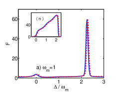
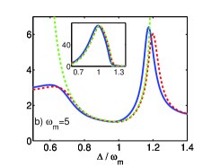
Figure 1: (Color online) Resonator Fano factor $F$ and average energy ${\left\langle n\right\rangle}$ (inset) as a function of $\Delta$ calculated using $P(B)$ (dashed red curves) and numerically (solid blue curves). In (a) $\omega_{m}=1$, $g=0.4$, $\gamma_{m}=5\times 10^{-5}$, and in (b) $\omega_{m}=5$, $g=1.5$, $\gamma_{m}=3\times 10^{-5}$, in each case $\bar{n}=0$ and $\Omega=0.05$ (we adopt units such that $\gamma_{c}=1$). The results obtained from the Gaussian approximation to $P(B)$ [see text] are shown in (b) (dashed green curves).

The Fokker-Planck equation equivalent to Eq. (8) has a steady-state solution $P(B)\propto{\rm exp}(-U(B))$, with

$$U(B) = \int\limits_{0}^{B}\frac{2B^{\prime}(\gamma_{m}+\gamma_{BA}(B^{\prime}))}{D_{m}+D_{BA}^{-}(B^{\prime})}{\rm{d}}B^{\prime},$$ (11)

where small corrections to the drift terms due to the noise have been neglected Lax ; LaxIX . This potential solution can be used to calculate the average resonator energy, ${\left\langle n\right\rangle}$ ($n=b^{\dagger}b$), and associated fluctuations over a wide range of parameters, including both the good and bad cavity limits. Figure 1 shows a comparison of ${\left\langle n\right\rangle}$, and the resonator Fano factor $F=({\left\langle n^{2}\right\rangle}-{\left\langle n\right\rangle}^{2})/{\left\langle n\right\rangle}$, obtained using the $P(B)$ distribution and the results of a direct numerical solution LKM of the master equation [Eq. (2)]. The numerical calculation is performed in a restricted number state basis using 3 states for the cavity and up to 120 for the resonator. We also neglect elements representing coherence between resonator states with a large separation in energy HRA . Representing the cavity in a basis centered on the equivalent uncoupled ($g\rightarrow 0$) state, i.e. $a^{\prime}=a+i\Omega/(\gamma_{c}/2-i\Delta)$, allowed us to study strongly driven cavities using only a few states (so long as the associated variance is not too large).

We see from Fig. 1 that there is very good agreement between the numerics and the calculation using Eq. (11) when the resonator is in a limit-cycle state (characterized in Fig. 1 by a large value of $\langle n\rangle$ and a relatively low Fano factor.) The agreement is still quite good fnote when the resonator undergoes a dynamical transition from the limit-cycle state back to one in which it fluctuates instead about a fixed point LKM ; CB ; HRA (marked by peaks in the Fano factor). The main approximation we have made is to neglect the higher-order derivatives (and hence higher-order correlations) by truncating the Wigner function. The relatively strong couplings we used in order to capture the limit-cycle dynamics numerically LKM provide a severe test of this approximation. The slight shift between the analytical and numerical curves in the figures is a sign that we are approaching the limits (in terms of coupling strengths) of the validity of this approach foot3 .

In a limit cycle the resonator distribution can be approximated as a Gaussian centered at an amplitude $B_{0}$, determined by the condition $\gamma_{m}=-\gamma_{BA}(B_{0})$, with a width given by $\sigma^{2}=(D_{m}+D_{BA}^{-}(B_{0}))/(2B_{0}\frac{{\rm{d}}\gamma_{BA}}{{\rm{d}}B}|_{B_{0}})$, and a Fano factor $F\approx 4\sigma^{2}$. The Gaussian approximations to $\langle n\rangle$ (given by $B_{0}^{2}-1/2$) and the Fano factor are compared with results from numerics and using the full $P(B)$ distribution in Fig. 1b.

The resonator Fano factor drops when it is in a well-defined limit-cycle state. In the highly idealised case where thermal noise is negligible ($\overline{n}\approx 0$), the cavity can drive the resonator into a non-classical sub-Poissonian state with $F<1$ (see Fig. 2). This is a consequence of the low noise properties of the cavity: it is well-known in the context of laser physics that regular pumping can lead to sub-Poissonian states WM . However, for a mechanical resonator thermal noise plays an important role and we now examine to what extent we can think of this being suppressed in the limit-cycle states. A useful comparison can be made between the cavity-driven resonator states and a displaced thermal state (DTS) with the same amplitude, thermal occupation number $\overline{n}$ and external damping $\gamma_{m}$. A DTS DTS is produced by harmonically driving a resonator initially in a thermal state, increasing its energy without introducing additional fluctuations. We choose a DTS for comparison as it reduces to a coherent state for $\bar{n}\to 0$, meaning it is both the generalization of a coherent state to finite $\bar{n}$ and of a thermal state to finite amplitude.

The Fano factor of a DTS with amplitude $B_{0}$ is $F_{d}=(\bar{n}(1+\bar{n})+(2\bar{n}+1)|B_{0}|^{2})/(\bar{n}+|B_{0}|^{2})$ and we compare this with that of the cavity-driven resonator in Fig. 2 for a range of external bath temperatures. In a well-defined limit cycle the value of the ratio $F/F_{d}$ is suppressed significantly below unity and we can think of the cavity as suppressing the thermal fluctuations. Note that this suppression also occurs outside the good cavity limit shown. As with the usual cavity induced cooling MCCG , the noise suppression occurs because the low-noise cavity can increase the friction (damping) on the resonator without adding significantly to the diffusion. Thus, driving a mechanical resonator via a cavity in this way produces a lower-noise state than driving with a perfect harmonic drive.

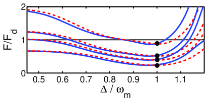
Figure 2: (Color online) Analytic [Eq. (11)] (dashed red curves) and numerical (solid blue curves) calculations of the resonator Fano factor $F$ in terms of $F_{d}$. The curves are (top to bottom) $\bar{n}=0,0.5,1,5$. In each case $\omega_{m}=5$, $\gamma_{m}=3\times 10^{-5}$, $g=2$ and $\Omega=0.05$. The dots represent the on-resonance value calculated using Eq. (12). Note, for $\bar{n}=0$, $F_{d}=1$ and $F$ reaches a minimum $\simeq 0.9$.

For $\Delta\sim\omega_{m}$ and in the good cavity limit, we can use Eqs. (6) and (11), together with the fact that $P(B)$ is almost Gaussian in a well-defined limit-cycle to obtain a simple approximate expression for the Fano factor,

$$F = \left(\bar{n}+1+\frac{g^{2}B_{0}^{2}}{4\omega^{2}_{m}}\right)\left[\frac{J_{1}(z)}{J_{1}(z)-zJ^{\prime}_{1}(z)}\right]_{z=gB_{0}/\omega_{m}},$$ (12)

where the amplitude $B_{0}$ is defined by $\gamma_{m}=-\gamma_{BA}(B_{0})$; the predictions of this equation are shown as dots in Fig. 2. This formula breaks down when the cavity-resonator coupling is increased sufficiently to allow the co-existence of more than one stable limit cycle MHG , (although it correctly predicts $F$ within the second limit cycle once the first has become unstable). Thus whilst Eq. (12) suggests that an arbitrarily small $F$ can always be achieved, the actual minimum value achievable for a given system is set by this expression together with the requirement that $\gamma_{m}=-\gamma_{BA}(B)$ has a single (non-zero) solution.

As well as fluctuations in amplitude, the resonator also undergoes phase diffusion which determines the linewidth in the limit-cycle state. In a well-defined limit-cycle, we can write a coarse-grained equation of motion for the phase Lax ; CB $\phi$, again linearizing the fluctuations,

$$B_{0}\dot{\phi} = i\eta_{T}^{+}+\delta\omega_{L}{\delta B}.$$ (13)

where $\delta B$ represents the amplitude fluctuations $B-B_{0}$ and $\delta\omega_{L}=B_{0}\frac{{\rm{d}}\delta\omega}{{\rm{d}}B}|_{B_{0}}$ is the frequency shift linearized about the limit cycle. Defining the phase diffusion in the same way as the amplitude diffusion, Eq. (9), we get,

$$D_{\phi} = \frac{1}{2B_{0}^{2}}\left(D_{m}+D_{BA}^{+}(B_{0})+\frac{4\delta\omega_{L}^{2}}{\gamma_{L}^{2}}(D_{m}+D_{BA}^{-}(B_{0}))\right)$$ (14)

where $\gamma_{L}=B_{0}\frac{{\rm{d}}\gamma_{BA}}{{\rm{d}}B}|_{B_{0}}$ is the linearized damping and cross-correlations have been neglected. Because the shift in the resonator frequency due to the cavity (optical spring effect) is amplitude dependent, the amplitude fluctuations can give rise to an important additional contribution to the phase diffusion. The phase diffusion is shown in Fig. 3 and it is clear that although the optical spring contribution is negligible at the center of the side band resonance (where $\delta\omega_{L}$ itself is negligible vah ), it nevertheless becomes important on either side.

Numerical calculations of the resonator spectrum $S(\omega)=\int dt{\rm e}^{-i\omega t}\langle\{b^{\dagger}(t),b(0)\}\rangle$ show near-Lorentzian peaks around $\omega=0$ and $\omega=\omega_{m}$ of width $\Lambda_{0}$ and $\Lambda_{\omega_{m}}$. These widths are determined by the slowest dissipative timescale at each frequency HRA ; Lax , and hence $\Lambda_{0}$ is given by the energy relaxation rate $\Lambda_{0}=\frac{B_{0}}{2}\frac{{\rm{d}}\gamma_{BA}}{{\rm{d}}B}\big{|}_{B_{0}}$ and the linewidth is given by the phase diffusion, $\Lambda_{\omega_{m}}=\frac{D_{\phi}}{2}$. There is good agreement between the numerical and analytic calculations of these quantities (Figs. 3 b,c) within the limit cycle regime (the main difference again an effective shift in $\Delta$).

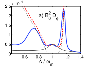
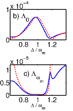
Figure 3: (Color online) a) Phase diffusion calculated numerically (solid blue) and analytically (dashed red). Solid and dashed thin lines show the direct phase diffusion $(D_{m}+D_{BA}^{+})/2$ and that due to the optical spring effect $2\delta\omega_{L}^{2}/\gamma_{L}^{2}(D_{m}+D_{BA}^{-})$ respectively. The insets show the linewidths $\Lambda_{0}$ (b) and $\Lambda_{\omega_{m}}$ (c). Parameters are: $\omega_{m}=5,\gamma_{m}=3\times 10^{-5},g=1.5,\Omega=0.05,\bar{n}=0$.

In conclusion, we have studied the amplitude and phase noise of limit-cycle states of a mechanical resonator driven by an optical cavity. Within a limit-cycle amplitude fluctuations are suppressed in the sense that they can be substantially less than in a corresponding state produced by simply applying a pure harmonic drive, the counterpart of the cooling that occurs in the stable regime. For low enough thermal noise the cavity generates non-classical sub-Poissonian resonator states. However, for the phase diffusion in the limit-cycle states the cavity noise simply adds to the effects of thermal fluctuations and the optical spring effect can also generate a significant contribution. The quantum noise of the resonator is described rather well by the truncated Wigner function approach over a range of resonator frequencies, both within the limit-cycle states and more surprisingly within the transition regions.

We thank T. Harvey for help with aspects of the numerics. This work was supported by EPSRC (UK).

References

- (1) M. Aspelmeyer and K. Schwab (eds.), Focus on Mechanical Systems at the Quantum Limit, New J. Phys. 10 095001 (2008).
- (2) S. Bose, K. Jacobs, and P. L. Knight, Phys. Rev. A 59, 3204 (1999); D. Vitali et al. J. Opt. Soc. Am. B 20, 1054 (2003); M. Blencowe, Phys. Rep. 395, 159 (2004).
- (3) V. Peano and M. Thorwart, Phys. Rev. B 70, 235401 (2004); I. Katz et al. Phys. Rev. Lett. 99, 040404 (2007).
- (4) A. Naik et al. Nature (London) 444 67 (2006); A. A. Clerk et al. arXiv:0810.4729; L. F. Wei et al. Phys. Rev. Lett. 97, 237201 (2006).
- (5) T. J. Kippenberg and K. J. Vahala, Science 321, 1172 (2008); I. Favero and K. Karrai, Nature Photon. 3, 201 (2009); F. Marquardt and S. M. Girvin, Physics 2 40 (2009).
- (6) I. Wilson-Rae et al. ibid. 99, 093901 (2007);F. Marquardt et al. Phys. Rev. Lett. 99 093902 (2007); C. Genes et al. Phys. Rev. A 77, 033804 (2008).
- (7) S. Gröblacher et al., Nature Phys. 5, 485 (2009); Y.-S. Park and H. Wang, ibid. 5, 489 (2009); A. Schliesser et al., ibid. 5, 509 (2009).
- (8) D. F. Walls and G. J. Milburn, Quantum Optics (Springer-Verlag, Berlin, 1994).
- (9) T. Carmon et al. Phys. Rev. Lett. 94, 223902 (2005); C. Metzger et al. ibid. 101, 133903 (2008).
- (10) F. Marquardt, J. G. E. Harris and S. M. Girvin, Phys. Rev. Lett. 96, 103901 (2006).
- (11) S.D. Bennett and A. A. Clerk, Phys. Rev. B 74, 201301 (2006).
- (12) T. J. Harvey, D. A. Rodrigues and A. D. Armour, Phys. Rev. B 78, 024513 (2008); T. J. Harvey, PhD Thesis (University of Nottingham, unpublished, 2009).
- (13) K. Vahala, et al., Nature Phys., 5, 682, (2009).
- (14) M. Ludwig, B. Kubala and F. Marquardt, New J. Phys. 10, 095013 (2008).
- (15) M. Lax, Phys. Rev. 160, 290 (1967).
- (16) M. Lax and W. Louisell, Phys. Rev. 185, 568 (1969).
- (17) K. J. Vahala, Phys. Rev. A 78, 023832 (2008).
- (18) For the parameters shown here, the shift .
- (19) The description works well even in the regime defined by , where the zero-point fluctuations of the resonator are comparable to the cavity induced fluctuations MHG .
- (20) H. Saito and H. Hyuga, J. Phys. Soc. Jap. 65, 1648 (1996).