3D models of radiatively driven colliding winds in massive O+O star binaries - III. Thermal X-ray emission

Abstract

The X-ray emission from the wind-wind collision in short-period massive O+O-star binaries is investigated. The emission is calculated from three-dimensional hydrodynamical models which incorporate gravity, the driving of the winds, orbital motion of the stars, and radiative cooling of the shocked plasma. Changes in the amount of stellar occultation and circumstellar attenuation introduce phase-dependent X-ray variability in systems with circular orbits, while strong variations in the intrinsic emission also occur in systems with eccentric orbits. The X-ray emission in eccentric systems can display strong hysteresis, with the emission softer after periastron than at corresponding orbital phases prior to periastron, reflecting the physical state of the shocked plasma at these times.

Our simulated X-ray lightcurves bear many similarities to observed lightcurves. In systems with circular orbits the lightcurves show two minima per orbit, which are identical (although not symmetric) if the winds are identical. The maxima in the lightcurves are produced near quadrature, with a phase delay introduced due to the aberration and curvature of the wind collision region. Circular systems with unequal winds produce minima of different depths and duration. In systems with eccentric orbits the maxima in the lightcurves may show a very sharp peak (depending on the orientation of the observer), followed by a precipitous drop due to absorption and/or cooling. We show that the rise to maximum does not necessarily follow a $1/d_{\rm sep}$ law. Our models further demonstrate that the effective circumstellar column can be highly energy dependent. Therefore, spectral fits which assume energy independent column(s) are overly simplified and may compromise the interpretation of observed data.

To better understand observational analyzes of such systems we apply Chandra and Suzaku response files, plus poisson noise, to the spectra calculated from our simulations and fit these using standard XSPEC models. We find that the recovered temperatures from two or three-temperature mekal fits are comparable to those from fits to the emission from real systems with similar stellar and orbital parameters/nature. We also find that when the global abundance is thawed in the spectral fits, sub-solar values are exclusively returned, despite the calculations using solar values as input. This highlights the problem of fitting oversimplified models to data, and of course is of wider significance than just the work presented here.

Further insight into the nature of the stellar winds and the WCR in particular systems will require dedicated hydrodynamical modelling, the results of which will follow in due course.

1 Introduction

The shock-heated plasma in the wind-wind collision region (WCR) of massive stellar binaries can produce copious X-ray emission. The emission often displays orbital variability, which can result from changes to the occultation of the emitting region by the stars, to the attenuation through the stellar winds, and to the separation of the stars (e.g. Rauw et al. 2002a; Schild et al. 2004; Sana et al. 2004; De Becker et al. 2006; Linder et al. 2006; Pollock & Corcoran 2006; Nazé et al. 2007; Hamaguchi et al. 2007; Sana et al. 2008). In wider systems, the post-shock plasma may exhibit signs of non-equilibrium ionization (Pollock et al. 2005), and non-equilibrium electron and ion temperatures (Zhekov & Skinner 2000).

The X-ray emission is a useful probe of the underlying wind parameters. The hardness of the emission is related to the post-shock temperatures within the WCR, which in turn depends on the pre-shock wind speed. The X-ray brightness depends on the pre-shock density of the winds, while the absorption of soft X-rays through the circumstellar environment depends on the integrated density along sight lines to the WCR (e.g. Stevens, Blondin & Pollock 1992, 1996; Pittard & Stevens 1997; Pittard et al. 1998; Pittard & Corcoran 2002; Parkin & Pittard 2008; Parkin et al. 2009). Hence both the brightness and the degree of absorption provide information about the stellar mass-loss rates. Although the X-ray emissivity is proportional to the square of the density, inhomogeneties can be rapidly smoothed out within adiabatic WCRs: thus the resulting X-ray emission may be relatively insensitive to the presence of clumps (Pittard 2007). Since mass-loss rate estimates are often uncertain due to unknown wind clumping factors, an insensitivity to clumping potentially allows the X-ray emission from CWBs to provide accurate determinations of stellar mass-loss rates. Recent observations in the UV have highlighted the uncertainty which still exists, with mass-loss rate estimates differing by factors of up to 100 with respect to other methods (e.g. Bouret, Lanz & Hillier 2005; Martins et al. 2005b; Fullerton, Massa & Prinja 2006). A recent review of the current situation can be found in Puls, Vink & Najarro (2008).

The WCR can also be a site of particle acceleration. The energetic particles produce non-thermal radio emission via the synchrotron process (e.g. Dougherty et al. 2003; Pittard et al. 2006), and non-thermal X-ray and $\gamma$-ray emission from inverse Compton cooling, neutral pion decay, and relativistic bremsstrahlung (Pittard & Dougherty 2006; Leyder et al. 2008). The non-thermal radio emission can sometimes be spatially resolved (e.g. Williams et al. 1997; Dougherty, Williams & Pollacco 2000b; Dougherty et al. 2005), and can also undergo dramatic variations in flux (e.g. Williams et al. 1992; White & Becker 1995; Rauw et al. 2002b; De Becker et al. 2004c; Blomme et al. 2005, 2007; Van Loo et al. 2008). If the particle acceleration efficiency is sufficiently high, the thermal structure of the WCR may be affected, resulting in softer X-ray emission as the plasma becomes cooler and denser. In this way the characteristics of the thermal X-ray emission may also constrain the efficiency of particle acceleration.

Models of the X-ray emission from colliding wind systems based on hydrodynamical simulations have, to date, been almost entirely performed in two-dimensions, with an underlying assumption of axissymmetry. While this approach is perfectly reasonable for wide systems with long orbital periods, axissymmetry is a poor assumption in shorter period systems where orbital effects become important. Though three-dimensional hydrodynamical simulations have been presented by Walder (1998) and Lemaster et al. (2007), these works also assumed that the winds were instantaneously accelerated to their terminal velocities. In reality, the winds in short-period systems collide prior to reaching their terminal velocities, so realistic simulations must also account for the acceleration of each wind. In a new advance, three-dimensional models with radiatively driven winds were recently presented by Pittard (2009a, hereafter Paper I). In addition to the acceleration of the winds, these models also account for orbital motion of the stars, gravity, and cooling in the post-shock plasma.

In this work we examine the thermal X-ray properties of the WCR from these models. We produce synthetic X-ray spectra and lightcurves, and examine how these change with the viewing angle. Section 2 describes details of the models and summarizes the method of calculating the X-ray emission and absorption. This section also notes the procedure adopted for folding the theoretical spectra through the response files of current X-ray observatories to simulate “fake” observations, which are subsequently fit using standard analysis techniques. We present our results in Section 3. Comparisons to previous numerical models and observations are made in Sections 4 and 5, respectively. Section 6 summarizes and concludes this work.

2 Details of the Calculations

2.1 The Numerical Models

The X-ray calculations in this paper are based on the three-dimensional hydrodynamical models described in Paper I. The models incorporate the radiative driving of the stellar winds (based on the Castor, Abbott & Klein (1975) formalism, with the finite disk correction factor of Pauldrach, Puls & Kudritzki (1986)), gravity, orbital effects, and cooling. The models were not designed to be of particular systems. Rather, the aim was to obtain a better understanding of how the nature of the collision region depends on various key parameters. The models are summarized in Tables 1 and 2. The assumption of main sequence stars minimizes the effects of tidal distortions, which are not modelled. The winds are also assumed to be spherically symmetric. Further details about the models can be found in Paper I.

Table 1: Assumed binary parameters for the models calculated in Paper I. The semi-major axis is $34.26\;\hbox{${\rm\thinspace R_{\odot}}$}$ in model cwb1, $76.3\;\hbox{${\rm\thinspace R_{\odot}}$}$ in models cwb2 and cwb3, and $55\;\hbox{${\rm\thinspace R_{\odot}}$}$ in model cwb4. $e$ is the orbital eccentricity and $\eta$ is the (terminal velocity) momentum ratio of the winds. $v_{\rm orb}$ and $v_{\rm w}$ are the orbital speeds of the stars and the preshock wind speeds along the line of centres. $\chi$ is the ratio of the cooling time to the characteristic flow time of the hot shocked plasma. $\chi\mathrel{\hbox to0.0pt{\lower 3.0pt\hbox{$\sim$}\hss}\raise 2.0pt\hbox{$<$}}1$ indicates that the shocked gas rapidly cools, while $\chi\mathrel{\hbox to0.0pt{\lower 3.0pt\hbox{$\sim$}\hss}\raise 2.0pt\hbox{$>$}}1$ indicates that the plasma in the WCR remains hot as it flows out of the system. Larger values of the ratio $v_{\rm orb}/v_{\rm w}$ produce a greater aberration angle, $\theta_{\rm ab}$, and tighter downstream curvature, of the WCR. The degree of downstream curvature of the WCR in the orbital plane is given by $\alpha_{\rm coriolis}$, where the curvature is assumed to trace an Archimedean spiral which in polar coordinates is described by $r=\alpha_{\rm coriolis}\theta$. The value of $\alpha_{\rm coriolis}$ corresponds to the approximate downstream distance (in units of $d_{\rm sep}$) along the WCR for each radian of arc it sweeps out in the orbital plane. Smaller values indicate tighter curvature. The leading and trailing arms of the WCR in model cwb3 display differing degrees of curvature, so the value quoted for this model is an average. The pre-shock orbital and wind speeds in model cwb3 are also different for each star/wind - the first (second) value is for the primary (secondary) star/wind. The values of $\chi$, $v_{\rm orb}/v_{\rm w}$, $\theta_{\rm ab}$ and $\alpha_{\rm coriolis}$ are phase dependent in model cwb4, because of its eccentric orbit - values at periastron and apastron are quoted. The values for $\alpha_{\rm coriolis}$ are calculated after comparing the orbital speeds at periastron and apastron against those in models cwb1 and cwb2, and represent the “instantaneous” curvature at these phases.

Model	Stars	Period	$e$	$\eta$	$v_{\rm orb}$	$v_{\rm w}$	$\chi$	$v_{\rm orb}/v_{\rm w}$	$\theta_{\rm ab}$	$\alpha_{\rm coriolis}$
		(d)			(${\rm{\rm\thinspace km}{\rm\thinspace s}^{-1}\,}$)	(${\rm{\rm\thinspace km}{\rm\thinspace s}^{-1}\,}$)			(∘)	($d_{\rm sep}\,{\rm rad}^{-1}$)
cwb1	O6V+O6V	3	0.0	1	290	730	0.34	0.40	17	3.5
cwb2	O6V+O6V	10	0.0	1	225	1630	19	0.14	$3-4$	6.5
cwb3	O6V+O8V	10.74	0.0	0.4	152,208	1800,1270	28,14	$0.16-0.084$	$\sim 2$	4.5
cwb4	O6V+O6V	6.1	0.36	1	$334-156$	$710-1665$	$0.34-19$	$0.47-0.09$	21-4	3-10

In model cwb1 two identical O6V stars move around each other in a circular orbit with a period of 3 days. The stellar separation is $34.26\;\hbox{${\rm\thinspace R_{\odot}}$}$, and each star has an orbital velocity $v_{\rm orb}=290\;\hbox{${\rm{\rm\thinspace km}{\rm\thinspace s}^{-1}\,}$}$. The thermal behaviour of the WCR can be described by the ratio of the cooling time to the characteristic flow time of the hot shocked plasma, $\chi\approx\frac{v_{8}^{4}d_{12}}{\hbox{${\dot{M}}$}_{-7}}$, where $v_{8}$ is the pre-shock wind speed in units of $1000\hbox{${\rm{\rm\thinspace km}{\rm\thinspace s}^{-1}\,}$}$, $d_{12}$ is the separation of the stars, and $\hbox{${\dot{M}}$}_{-7}$ is the stellar mass-loss rate in units of $10^{-7}\hbox{${\rm\hbox{${\rm\thinspace M_{\odot}}$}{\rm\thinspace yr}^{-1}\,}$}$ (c.f. Stevens et al. 1992). In model cwb1, the WCR is highly radiative ($\chi<<1$), and significantly distorted by orbital effects, showing strong aberration and downstream curvature. Model cwb1 is similar to many real systems, including HD 215835 (DH Cep; see Linder et al. 2007, and references therein), HD 165052 (Arias et al. 2002; Linder et al. 2007), and HD 159176 (De Becker et al. 2004b; Linder et al. 2007). All of these systems have near identical main-sequence stars of spectral type O6$-$O7, and circular or near-circular orbits with periods near 3 days.

In model cwb2 the orbital period is increased to 10 days, with the stellar separation becoming $76.3\;\hbox{${\rm\thinspace R_{\odot}}$}$. The winds collide at significantly higher speeds than in model cwb1, and the postshock gas is largely adiabatic. The aberration and downstream curvature of the WCR are both lessened compared to model cwb1. Model cwb2 is similar to HD 93161A, an O8V + O9V system with a circular orbit and an orbital period of 8.566 days (Nazé et al. 2005), albeit with slightly more massive stars and powerful winds. Another system which is not too dissimilar in its properties is Plaskett’s star (Linder et al. 2006, 2008), though this object contains stars which have evolved off the main sequence.

Model cwb3 examines the interaction of unequal winds in a hypothetical O6V+O8V binary. The stars in this model have the same separation as those in model cwb2. The primary wind collides at higher speed than the secondary wind, and its postshock plasma is slightly more adiabatic.

Model cwb4 investigates the effect of an eccentric orbit which takes the stars through a separation of $34.26-76.3\;\hbox{${\rm\thinspace R_{\odot}}$}$ (i.e. the separations of the stars in the circular orbits of models cwb1 and cwb2). The WCR is radiative at periastron and adiabatic at apastron, and the aberration and downstream curvature are phase dependent. A surprising finding from Paper I is that dense cold clumps formed in the WCR at periastron persist near the apex of the WCR until almost apastron. This is because the clumps have relatively high inertia, and flow out of the system much more slowly than the hotter gas which streams past them. Some well-known O+O binaries with eccentric orbits include (in order of increasing orbital period) HD 152248 ($e=0.127$; Sana et al. 2004), HD 93205 ($e=0.46$; Morrell et al. 2001), HD 93403 ($e=0.234$; Rauw et al. 2002a), Cyg OB2#8A ($e=0.24$; De Becker, Rauw & Manfroid 2004; De Becker et al. 2006) and $\iota$ Orionis ($e=0.764$; Bagnuolo et al. 2001).

2.2 Modelling the X-ray emission and absorption

To calculate the X-ray emission we read our hydrodynamical models into a radiative transfer ray-tracing code, and calculate appropriate emission and absorption coefficients for each cell using the temperature and density values. A synthetic image on the plane of the sky is then generated by solving the radiative transfer equation along suitable lines of sight through the grid. Since non-equilibrium effects are small in short period O+O systems (see Paper I), the X-ray emissivity is calculated using the mekal emission code (Mewe et al. 1995, and references therein) for optically thin thermal plasma in collisional ionization equilibrium. Solar abundances (Anders & Grevesse 1989) are assummed throughout this work. The emissivity is stored in look-up tables containing 200 logarithmic energy bins between $0.1-10\;$keV, and 91 logarithmic temperature bins between $10^{4}-10^{9}\;$K. Line emission dominates the cooling at temperatures below $10^{7}\;$K, with thermal bremsstrahlung dominating at higher temperatures. The hydrodynamical grid is large enough to capture the majority of the X-ray emission from each of the models.

The main contributors to the absorption of keV X-rays are the K shells of the CNO elements. The photoelectric absorption is calculated using Cloudy (Ferland 2000). The opacity is stored in look-up tables containing 26 temperatures between $10^{4}-10^{9}\;$K. As in previous works (e.g. Luo, McCray & Mac Low 1990; Stevens, Blondin & Pollock 1992; Myasnikov & Zhekov 1993; Pittard & Stevens 1997), electron scattering is neglected. Electron scattering becomes important once the optical depth to this process nears unity, i.e. when $\tau_{\rm e}=N_{\rm e}\sigma_{\rm e}\mathrel{\hbox to0.0pt{\lower 3.0pt\hbox{$\sim$}\hss}\raise 2.0pt\hbox{$>$}}1$, where $N_{\rm e}$ is the column density of free electrons along a line of sight and $\sigma_{\rm e}$ is the Thomson cross-section. In the ionized winds, the proton and electron column densities are approximately equal. In our models, $\tau_{\rm e}<1$ is indeed satisified. For example, in the dense circumstellar environment of model cwb1, an observer viewing the system pole on ($i=0^{\circ}$) sees an average “effective” hydrogen column density to high energy ($2-10\,$keV) X-rays of $\approx 2\times 10^{22}\,{\rm cm^{-2}}$ (see Fig. 5(a) and Section 3.1.3 for further details). Since occulation is minimal, the “effective” column density in this case reflects the true column density of the circumstellar environment. The electron scattering optical depth is then $\tau_{\rm e}\approx 0.13$. Note that the higher “effective” column densities shown in Fig. 5(a) for an observer in the orbital plane ($i=90^{\circ}$) at phase 0.0 are instead a reflection of the occultation that takes place at this time, and do not indicate that electron scattering becomes optically thick (see Section 3.1.3 for further details). Electron scattering will, however, be important in systems with denser winds, where very high column densities can be reached. Such systems, include, for example, the supermassive system $\eta$ Car (see, e.g., Parkin et al. 2009). The likely effect is that abrupt changes in the emission (e.g. in lightcurves and spectra) will be somewhat smoothed/blurred, though we leave a study of this effect to future work.

The present calculations also have an interstellar absorption column of $10^{21}\;{\rm cm^{-2}}$ added to them, and each model is assumed to be at a distance of 1 kpc from an observer. The X-ray spectra/lightcurves were calculated from a single “frame” (i.e. changing the orientation) for the circular orbit models (cwb1, cwb2, and cwb3), and from a sequence of snapshots for the eccentric model (cwb4). The lightcurve for $i=0^{\circ}$ is invariant for models cwb1, cwb2, and cwb3.

2.3 Generating and analyzing “fake” spectra

In the following section we “observe” the theoretical spectra generated from our ray-tracing code with the Chandra and Suzaku X-ray observatories. This involves convolving the theoretical spectra with the energy response and effective area of these telescopes, to generate spectra in counts/energy bin. Counting statistics are included in this process. The resulting “fake” spectra are then analyzed using XSPEC, and fitted with standard spectral models, in an analogous manner to the analysis of real data (the only difference is that a background component does not need to be subtracted). The aim is to study how the fit parameters compare with those from the analysis of real data, and how they compare to what is known about the theoretical input spectra. This type of analysis remains very novel, having been applied to colliding wind binaries only by Stevens et al. (1996), Pittard & Stevens (1997), Zhekov & Skinner (2000), and Pittard & Corcoran (2002).

The majority of our analysis is concentrated on simulated Suzaku XIS spectra. To generate these we used the XIS0 ancillary response file (ARF) and redistribution matrix file (RMF) for an on-axis point source downloaded from the HEASARC website. Although these are old (2006) calibrations, they are fine for our purpose, which is to investigate the values and variation of the best-fit parameters, and the corresponding fluxes of the best-fit models. A small number of simulated Chandra ACIS-I spectra were also computed. These used the Cycle 11 ACIS-I aimpoint ARF and RMF, downloaded from the Chandra website.

The spectra were binned with the FTOOLS task grppha so that each energy bin contained a minimum of 20 counts. The “fake” spectra were fitted using XSPEC version 12.5.0ac, distributed with HEASoft6.6.3. Since an ISM column of $10^{21}\,{\rm cm^{-2}}$ was added to our theoretical spectra, we force the absorbing column to each model component to be at least as large. However, we note that if this restriction is relaxed, the best fit often returned lower columns. The theoretical spectra were generated using emissivities from the mekal thermal emission code, so for consistency we also fit the data in XSPEC using the mekal thermal model.

Table 2: Assumed stellar parameters for the models.

Parameter/Star	O6V	O8V
Mass (${\rm\thinspace M_{\odot}}$)	30	22
Radius (${\rm\thinspace R_{\odot}}$)	10	8.5
Effective temperature (K)	38000	34000
Mass-loss rate (${\rm\hbox{${\rm\thinspace M_{\odot}}$}{\rm\thinspace yr}^{-1}\,}$)	$2\times 10^{-7}$	$10^{-7}$
Terminal wind speed (${\rm{\rm\thinspace km}{\rm\thinspace s}^{-1}\,}$)	2500	2000

3 Results

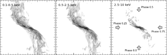
Figure 1: Broad-band intensity images from model cwb1 at $i=0^{\circ}$. From left to right the images are in the $0.1-0.5$ keV, $0.5-2.5$ keV, and $2.5-10$ keV bands. The grayscale covers 4 orders of magnitude in brightness, with black corresponding to a maximum intensity of $10^{7}\,{\rm erg\,cm^{-2}\,s^{-1}\,keV^{-1}\,ster^{-1}}$ in the left and right panels, and $10^{8}\,{\rm erg\,cm^{-2}\,s^{-1}\,keV^{-1}\,ster^{-1}}$ in the central panel. The major ticks on each axis mark out 0.2 mas. The stars are at $\pm 0.08$ mas north and south of the image centre. The arrows mark the direction in which an observer looks into the system at the indicated orbital phases. We also define an azimuthal viewing angle, $\phi$, which increases anti-clockwise from the bottom of the image, so that at phase 0.0 $\phi=0^{\circ}$. $\phi=90^{\circ}$ corresponds to phase 0.75, and $\phi=180^{\circ}$ and $\phi=270^{\circ}$ correspond to phases 0.5 and 0.25, respectively.

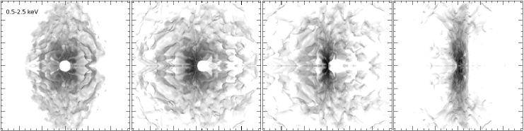
Figure 2: Broad-band 0.5-2.5 keV intensity images from model cwb1 at $i=90^{\circ}$. From left to right the phase of the observation increases from 0.0 (conjunction, $\phi=0^{\circ}$), to 0.125 ($\phi=315^{\circ}$), to 0.25 (quadrature, $\phi=270^{\circ}$), to 0.375 ($\phi=225^{\circ}$). The grayscale covers 4 orders of magnitude in brightness, with black corresponding to a maximum intensity of $10^{8}\,{\rm erg\,cm^{-2}\,s^{-1}\,keV^{-1}\,ster^{-1}}$. The major ticks on each axis mark out 0.2 mas.

3.1 Model cwb1

3.1.1 Images

Fig. 1 shows broad-band images from model cwb1 for an observer located directly above the orbital plane ($i=0^{\circ}$). The stars are oriented north-south in these images (cf. the images of the thermal radio emission in Pittard 2009b, hereafter Paper II), and the orbital induced aberration and downstream curvature of the WCR is clearly visible. The emission morphology reflects the underlying structure and clumpiness of the WCR, resulting from the powerful dynamical instabilities present in this system. A detailed discussion of the hydrodynamics can be found in Paper I. The projected emission from different inhomogeneities merges together near the apex of the WCR, but individual clumps and bowshocks can be identified further downstream. It is clear that a small amount of emission, particularly at the lowest energies, is not captured due to the finite extent of the hydrodynamical grid used in the model, but this loss should not be significant. The hard ($2-10$ keV) emission predominantly arises from the apex of the WCR. Although there are regions of hot gas further downstream (see Paper I), the density there is too low for these regions to contribute significantly to the emission. The spatial scale of the emission is far too small to be resolved with current X-ray telescopes: WR 147 is likely to remain the only system with a spatially resolved WCR (Pittard et al. 2002c) for some time to come.

Fig. 2 shows broad-band images from model cwb1 for an observer located in the orbital plane ($i=90^{\circ}$). The clumpy nature of the WCR and the bowshocks around some of the denser regions are visible. At particular phases/viewing angles the emission from bright parts of the WCR is occulted by the foreground star. Additional foreground emission is sometimes seen in front of the stellar disc at these moments.

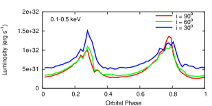
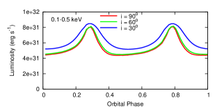
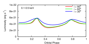
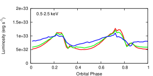
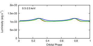
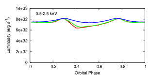
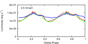
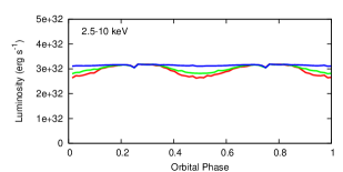
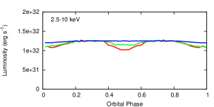
Figure 3: X-ray lightcurves for models cwb1 (left), cwb2 (middle), and cwb3 (right), calculated over the energy bands $0.1-0.5\;$keV (top), $0.5-2.5\;$keV (middle), and $2.5-10\;$keV (bottom) for inclination angles $i=30^{\circ},60^{\circ}$ and $90^{\circ}$. In all cases, the observer is located along a direction vector specified by $\phi=0^{\circ}$ (i.e. the longitude of periastron, $\omega=270^{\circ}$). The stars are at conjunction at phases 0.0 and 0.5, and quadrature at phases 0.25 and 0.75.

3.1.2 Lightcurves

Lightcurves from model cwb1, computed over the energy bands $0.1-0.5\;$keV, $0.5-2.5\;$keV, and $2.5-10\;$keV, are shown in the left column of Fig. 3. The stars pass in front of each other at phases 0.0 and 0.5, and are at quadrature at phases 0.25 and 0.75. As the orbit is circular, the intrinsic emission is constant, so the variations displayed in the lightcurves in Fig. 3 are entirely due to changes in the occultation and circumstellar absorption as a function of phase. If there were no orbital induced effects on the WCR (i.e. no aberration or curvature of the WCR), the lightcurves would display dual symmetry about phases corresponding to both quadrature (0.25, 0.75) and conjunction (0, 0.5) of the stars to the line of sight (c.f. Pittard & Stevens 1997; Antokhin, Owocki & Brown 2004), because of the equal winds and constant stellar separation. When orbital effects are included, the symmetry about quadrature is broken, and the lightcurves instead are expected to show a double periodicity in the case of identical winds. However, close examination of Fig. 3 reveals that in fact this dual periodicty is also broken (note that the peaks in the $0.1-0.5\;$keV lightcurve have different heights). Clearly, the dynamical instabilities which form in the WCR develop independently in each arm, and break this symmetry too.

The variation of flux with orbital phase is largest in all lightcurves when the inclination angle $i=90^{\circ}$, and decreases with decreasing $i$. The amplitude of variation is also largest in the softest band. Both of these findings are expected: the soft emission is more easily absorbed by the stellar winds, while lines of sight to the WCR pass, on average, through a greater attenuation column, and there is also greater occultation of the emission region by the stars, when the observer is in the orbital plane.

Minima in the lightcurves occur near phases 0.0 and 0.5, when the emission from the WCR suffers the greatest reduction by stellar occultation and wind absorption. However, close examination reveals that the minima actually occur slightly before each conjunction. This reflects the aberration of the WCR. In model cwb1 the abberation angle is $\approx 17^{\circ}$, which corresponds to 0.05 in orbital phase, and is therefore similar to the observed lead.

Short, sharp dips are also seen in the lightcurves near orbital phases 0.32 and 0.82 (being most visible in the $0.5-2.5$ keV lightcurve for $i=90^{\circ}$). This is due to absorption from the thin dense layer of cooled post-shock gas (see Paper I). The dips are similar to those seen in Fig. 15 of Antokhin et al. (2004), but are broader and less obvious due to the orbital-induced curvature of the WCR. They also display a phase lead consistent with the phase lead of the main minima.

The ISM corrected $0.5-10$ keV luminosity is $6.75\times 10^{32}\,\hbox{${\rm{\rm\thinspace erg}{\rm\thinspace s}^{-1}\,}$}$, $1.41\times 10^{33}\,\hbox{${\rm{\rm\thinspace erg}{\rm\thinspace s}^{-1}\,}$}$, and $6.54\times 10^{32}\,\hbox{${\rm{\rm\thinspace erg}{\rm\thinspace s}^{-1}\,}$}$ at viewing angles of $(i,\phi)=(90^{\circ},0^{\circ})$, $(90^{\circ},90^{\circ})$, and $(0,0)$ (pole-on), giving $L_{\rm x}/L_{\rm bol}=4.7\times 10^{-7}$, $9.9\times 10^{-7}$, and $4.6\times 10^{-7}$, respectively. These values are all significantly above the scaling law (log $L_{\rm x}/L_{\rm bol}$)$=-6.912\pm 0.153$) determined by Sana et al. (2004), and are thus indicative of a binary system with strong colliding winds emission.

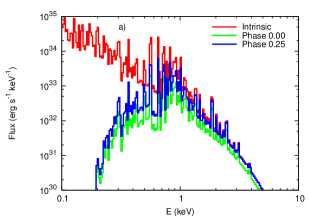
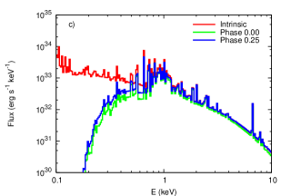
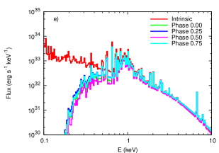
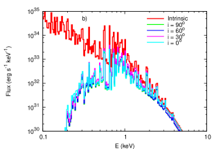
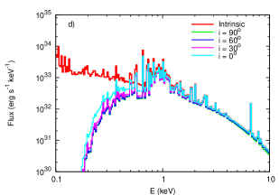
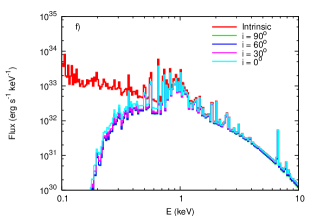
Figure 4: (Top) X-ray spectra from models cwb1 (left), cwb2 (middle), and cwb3 (right) for an observer in the orbital plane ($i=90^{\circ}$) as a function of orbital phase. (Bottom) As top but as a function of $i$ for an observer with $\phi=0^{\circ}$.

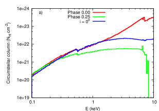
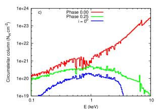
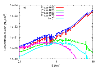
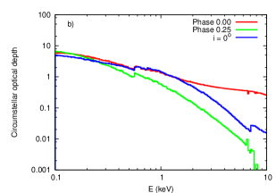
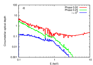
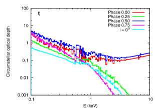
Figure 5: “Effective” circumstellar column (top) and optical depth (bottom) from models cwb1 (left), cwb2 (middle), and cwb3 (right) for an observer in the orbital plane ($i=90^{\circ}$) as a function of energy and orbital phase. The circumstellar column and optical depth for an observer at $i=0^{\circ}$ are also shown. Note that in some cases the “effective” column can be strongly weighted by occultation effects - at these times it is not a good indicator of the actual circumstellar column that the observed X-rays travel through.

3.1.3 Spectra

The emission from model cwb1 is overall very soft, reflecting the rapid cooling of the hot plasma in the WCR. Fig. 4(a) displays synthetic X-ray spectra as a function of orbital phase for an observer in the orbital plane. The spectra at phase 0.5 and 0.75 are almost identical to those at phase 0.0 and 0.25, differing only due to the time dependence of the dynamic instabilities present in each arm of the WCR, and so are not shown. The hard emission is lower at conjunction (phases 0.0 and 0.5) when one of the stars passes in front of the apex of the WCR, than at quadrature (phases 0.25 and 0.75). This is a combination of occultation and wind absorption, with the former dominating at hard energies (see below). The softer emission is also reduced at these phases as it is attenuated by a greater amount of unshocked stellar wind between the WCR and the observer. In contrast, at quadrature the emission suffers less attenuation and occultation, and it more easily escapes the system. Fig. 4(b) shows that the variation of the soft emission with the inclination angle, $i$, is small. The soft emission arises from relatively low temperature plasma, comprising a relatively large volume of the WCR. Consequently the loss of flux due to circumstellar absorption and stellar occultation is relatively independent of the orientation. As we shall see, interstellar absorption is a large contribution to the overall absorption of soft X-rays.

The variation of the hard emission with $i$ (see Fig. 4b) is of a similar magnitude to the change between conjunction and quadrature when the observer is in the orbital plane (see Fig. 4a). This is not surprising since in both cases the variation is mainly due to changes in the occultation, and these changes are comparable: more of the apex of the WCR is revealed as the observer’s sight line moves away from the eclipse at $i=90^{\circ}$, $\phi=0^{\circ}$.

Figs. 5(a) and (b) show the “effective” circumstellar column and optical depth as a function of energy for an observer in the orbital plane. These were calculated by comparing the ray-traced intrinsic and attenuated spectra (the latter prior to the addition of the interstellar column). Their ratio gives an energy dependent optical depth (Fig. 5b), which can be converted into an “effective” column (Fig. 5a) by considering the energy dependent opacity of the cold plasma in the winds. Note that this “effective” column does not always provide a good measure of the circumstellar column for an observed X-ray, since it can be substantially weighted by occultation effects (see below). Instead it is intended as an indicator of how realistic the usual method of using energy-independent columns with, for example mekal fits, is.

In Fig. 5(a) we see that the circumstellar column from the phase 0.0 calculation monotonically increases with energy (except at a few noteable absorption edges), reflecting the fact that the hardest emission is on average generated closest to the stars (see Fig. 1). The effective attenuation resulting from circumstellar absorption and stellar occultation exceeds that due to interstellar absorption (assumed to be $N_{\rm H}=10^{21}\,{\rm cm^{-2}}$) at energies above 0.2 keV. The effective circumstellar column exceeds $10^{23}\,{\rm cm^{-2}}$ for $E\mathrel{\hbox to0.0pt{\lower 3.0pt\hbox{$\sim$}\hss}\raise 2.0pt\hbox{$>$}}4$ keV. Columns this high cannot be produced by the winds themselves, and instead indicate substantial occultation of the intrinsic emission by the stars. The strong energy dependence of the column at phase 0.0 as shown in Fig. 5(a) also hints at weaknesses that are inherent in simple analyses of X-ray data of colliding wind binaries in which energy-independent columns are applied in model fits. While individual columns to multiple emission components clearly provide some level of energy-dependent $N_{\rm H}$, this is of course achieved in a rather crude and clumsy way.

The equivalent optical depth from circumstellar absorption and occultation is shown in Fig. 5(b). It is highest at the lowest energies. At phase 0.0, the optical depth $\tau=6$ at 0.1 keV, dropping to $\tau=0.26$ at 10 keV. In comparison, the ISM column provides an optical depth of 30 at 0.1 keV, declining to $10^{-3}$ at 10 keV.

Occultation of the harder X-ray emission is much reduced at phase 0.25 (see the spectrum in Fig. 4a), and this is manifest as a marked drop in the “effective” circumstellar column and optical depth values in Figs. 5(a) and (b). In fact, the column is now roughly constant over the energy range $0.5-7$ keV. In this case a simple analysis using energy-independent columns would probably not be too bad an approximation at this phase. However, it is clear that such analyses have major short-comings in short period binaries at phases when occultation is likely to be significant (for instance, the intrinsic luminosity can be significantly underestimated - see the following section). At the very highest energies ($E\mathrel{\hbox to0.0pt{\lower 3.0pt\hbox{$\sim$}\hss}\raise 2.0pt\hbox{$>$}}7$ keV) the effective circumstellar column again declines. This is due to the fact that the highest temperature plasma exists in localized bowshocks around clumps far downstream in the WCR, as discussed in Paper I.

Figs. 4(a) and (b) also show the effective circumstellar column and optical depth for an observer directly above/below the centre of mass in the orbital plane (i.e. at an inclination angle $i=0^{\circ}$). The degree of absorption and occultation are intermediate between the conjunction and quadrature phases of an observer in the orbital plane.

The deduced values of the energy-dependent circumstellar column shown in Fig. 5(a) can be compared to analytical estimates. Using Eq. 11 in Stevens et al. (1992), which gives the column density at quadrature from the stagnation point (assumed to be on the line of centres in the axisymmetric case) through the undisturbed terminal speed wind, we obtain $N_{\rm H}\sim 3.4\times 10^{21}\,{\rm cm^{-2}}$. While this is in good agreement with the column to the higher energy emission (which should be the best proxy to the apex of the WCR) at phase 0.25 (see Fig. 5a), it would seem to be a somewhat fortuitous coincidence. For instance, Stevens et al. (1992) note that under the assumption of axisymmetry the column at quadrature is independent of the system inclination. However, Fig. 5(a) shows that the circumstellar column for a pole-on observer ($i=0^{\circ}$) is significantly greater at most energies than the phase 0.25 column. This is because with equal strength winds all the material along the line-of-sight from the apex of the WCR to an observer at $i=0^{\circ}$ has been processed through the WCR, and is denser than the surrounding unshocked winds. In contrast, the line-of-sight to an observer in the orbital plane at phase 0.25 passes mostly through unshocked wind material. So there are actually large differences in the density structure along these two sightlines, yet this is not accounted for in Eq. 11 of Stevens et al. (1992).

Figure 6: Fits to “fake” spectra from the models for different viewing angles. a) Two-temperature fit to a fake Chandra spectrum of model cwb1 at $i=90^{\circ}$ and phase 0.0 (conjunction). b) As a) except the system is viewed at quadrature (phase 0.25). c) Three-temperature fit to a fake Chandra spectrum of model cwb2 for an observer in the orbital plane viewing the system at conjunction (phase 0.0). d) As c) except to a fake Suzaku spectrum. Note the much better spectral resolution in the Suzaku spectrum. The spectra in panels a)-d) have effective “exposures” of 10 ksec. e) Three-temperature fit to a fake Suzaku spectrum of model cwb3 for an observer in the orbital plane viewing the system at phase 0.0 (weaker O8V wind in front). f) As e) but at phase 0.5 (stronger O6V wind in front). Note the difference in the strength of the Fe K line. The spectra in panels e) and f) have effective “exposures” of 20 ksec.

3.1.4 Spectral fits

In this section we “observe” the theoretical spectra generated from model cwb1 with the Chandra and Suzaku X-ray observatories. Table 3 notes the results of the subsequent spectral fits, where an exposure time of 10 ksec has been assumed. At least three mekal components are needed to obtain satisfactory fits to the simulated Suzaku spectra, while the simulated Chandra spectra require at least two mekal components.

Fig. 6(a) shows the fake Chandra spectrum from model cwb1 at $i=90^{\circ}$ and phase 0.0, with Poisson statistics added. A single temperature wabs(mekal) model is a very poor fit to the simulated data ($\chi^{2}_{\nu}=3.91$). However, an acceptable fit is achieved with the addition of another mekal component ($\chi^{2}_{\nu}=1.27$). Fig. 6(b) shows the corresponding spectrum and fit at phase 0.25. The hotter temperature component has a slightly reduced temperature, a higher absorbing column, and a lower normalization at phase 0.0 (conjunction) compared to phase 0.25 (quadrature), in line with expectations (see Figs. 4a and 5a).

Two mekal components return reasonable fits to simulated Suzaku spectra with an exposure time of 10 ksec ($\chi^{2}_{\nu}=1.37$, at phase 0.0 when $i=90^{\circ}$), but fail to provide a good fit when the exposure time is increased to 40 ksec ($\chi^{2}_{\nu}=1.64$), notably failing to fit the line at 0.55 keV. Adding a third mekal component does not significantly improve the fit ($\chi^{2}_{\nu}=1.50$). Irrespective of the orbital phase, the temperatures of the three mekal components are all below 0.75 keV, reflecting the relatively cool shocked plasma created by the relatively low preshock wind speeds in this model. Furthermore, the best-fit absorbing columns are often significantly higher than the ISM value, indicating that the circumstellar absorption of X-rays is significant in this model.

The circumstellar columns returned from the spectral fits are consistent with the trend shown in Fig. 5(a) of higher effective column with energy. Also of note is that the derived $N_{\rm H}$ to the hottest mekal component of the spectral models is greater at phase 0.0 (conjunction) than at phase 0.25 (quadrature). In addition, the hottest mekal component is both hotter and brighter at phase 0.25. These are consistent with the changes to the circumstellar absorption and stellar occultation of the WCR with the orientation of the observer, as noted earlier.

A good fit to the simulated Chandra spectrum can also be obtained with a single mekal component if the global metal abundance is allowed to vary. In this case, a metal abundance of $0.13^{+0.01}_{-0.02}\,Z_{\odot}$ provides a good fit ($\chi^{2}_{\nu}=1.11$) to the data. This is very interesting, since we know that the actual plasma has solar abundances. Clearly, there is great opportunity for the analysis of low spectral resolution data to return unphysical fit parameters when fitting emission from inherently multi-temperature plasma with simpler (e.g. single temperature) spectral models. In an identical (10 ksec) analysis to a fake Suzaku spectrum we again find that a single temperature fit is very poor ($\chi^{2}_{\nu}=2.69$), but this time it remains poor ($\chi^{2}_{\nu}=2.13$) when the global metal abundance is allowed to vary (fitting at $z=0.079\pm 0.011\,Z_{\odot}$). This nicely illustrates the advantage of having higher spectral resolution. The story is more complicated for fits with two mekal components. Tying the global abundances of the mekal components together, one finds that the returned value from the analysis of the phase 0.0 fake Chandra spectrum is very poorly constrained, with its value depending on how the model approaches its minimum (e.g. the initial values entered into the model). The 90 per cent confidence interval typically extends from metallicities of $0.4-2.0\times$ solar, with a “best-fit” value of $z=0.79\,Z_{\odot}$. A three-temperature fit to the fake Suzaku phase 0.25 spectrum returns a global abundance of $z=0.71\,Z_{\odot}$ (since $\chi^{2}_{\nu}>2$, the uncertainty on this value cannot be estimated using the “error” command in XSPEC). It would therefore appear that the fits return more accurate abundances the more complex the spectral model is. These findings agree with the earlier work of Strickland & Stevens (1998) who were examining ROSAT data in a related context.

Table 4 shows the intrinsic luminosity of model cwb1, plus the intrinsic luminosity returned from the spectral fits (i.e. the observed luminosity, corrected for the interstellar and circumstellar absorption determined by the fit). We find that the intrinsic luminosities returned from the fits in all cases underestimate the true intrinsic luminosity from the system, by factors of up to 2. This discrepancy arises because direct occultation of the emission is a significant factor in close binaries like cwb1, yet no account is made for occultation in the fits. It again highlights problems which can ensue when fitting too-simple models to data. The discrepancy is larger at conjunction than at quadrature, as expected. We further note that the size of the discrepancy is not dependent on the resolution of the two spectra (i.e. Chandra versus Suzaku). The discrepancy reduces in wider systems (see model cwb2, next), but could be even larger in yet closer systems.

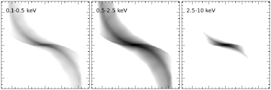
Figure 7: Broad-band intensity images from model cwb2 at $i=0^{\circ}$. From left to right the images are in the $0.1-0.5$ keV, $0.5-2.5$ keV, and $2.5-10$ keV bands. The maximum intensity in the images is $10^{7}\,{\rm erg\,cm^{-2}\,s^{-1}\,keV^{-1}\,ster^{-1}}$, and the grayscale covers 4 orders of magnitude in brightness. The major ticks on each axis mark out 0.5 mas. The stars are located north and south of the image centre by 0.18 mas.

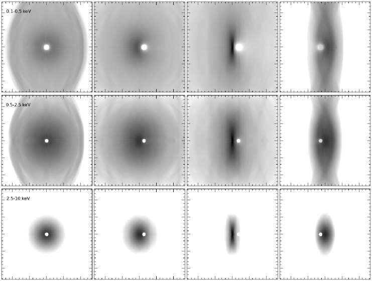
Figure 8: Broad-band intensity images from model cwb2 at $i=90^{\circ}$. From top to bottom the images are in the $0.1-0.5$ keV, $0.5-2.5$ keV, and $2.5-10$ keV bands. From left to right the phase of the observation increase from 0.0 (conjunction, $\phi=0^{\circ}$), to 0.125 ($\phi=315^{\circ}$), to 0.25 (quadrature, $\phi=270^{\circ}$), to 0.375 ($\phi=225^{\circ}$). The maximum intensity in the $0.1-0.5$ keV images is $10^{6}\,{\rm erg\,cm^{-2}\,s^{-1}\,keV^{-1}\,ster^{-1}}$, while in the $0.5-2.5$ keV, and $2.5-10$ keV images it is $10^{7}\,{\rm erg\,cm^{-2}\,s^{-1}\,keV^{-1}\,ster^{-1}}$. The grayscale covers 4 orders of magnitude in brightness, and the major ticks on each axis mark out 0.5 mas.

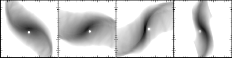
Figure 9: Broad-band $0.5-2.5$ keV intensity images from model cwb2 at $i=30^{\circ}$. From left to right the orbital phases are 0.0, 0.125, 0.25, and 0.375. The stars and the WCR again rotate anti-clockwise, while the maximum intensity of the images is $10^{7}\,{\rm erg\,cm^{-2}\,s^{-1}\,keV^{-1}\,ster^{-1}}$, and the major ticks on each axis mark out 0.5 mas.

3.2 Model cwb2

3.2.1 Images

Fig. 7 shows the broad-band intensity images from model cwb2 for an observer located directly above/below the orbital plane. The hardest emission is again confined to a region close to the apex of the WCR, and the curved shape of the WCR is clearly seen. The leading edge of each arm of the WCR is sharper and more distinct. The trailing edge is blurred because the hot plasma inside the WCR displays an increasing phase lag as one goes further from the orbital plane. This reflects the fact that the motion of this plasma is strongly influenced by the prior (rather than the current) positions of the stars. The extent of the low surface brightness emission from the WCR is affected by the size of the numerical grid. Calculations with a bigger grid would reveal that, for instance, the left-hand edge of the emission in the bottom right corner of the $0.5-2.5$ keV image in Fig. 7 would extend further to the left. However, we remain confident that the majority of the emission is captured in this (and the other) models, since the surface brightness is 4 orders of magnitude lower than the peak surface brightness obtained at the apex of the WCR.

Broad-band intensity images from model cwb2 for an observer in the orbital plane are shown in Fig. 8. The images bear substantial similarities to the radio images shown in Paper II. The morphology of these images is determined by the relative orientation of the observer to the WCR and the stars. The foreground star eclipses the emission from those parts of the WCR which lie behind it. The double-helix-like structure seen in the soft and medium-band images when the system is half-way between conjunction and quadrature (at phase 0.375) is due to limb-brightened emission. The vertical curvature again illustrates the increasing phase-lag of the shocked gas with distance above/below the orbital plane. The increasing confinement of emission to the apex of the WCR at higher energies means that the hard-band images instead show a disc-like structure. In all 3 energy bands the surface brightness of the emission is highest in the images generated at quadrature, when the X-rays from the apex of the WCR initially escape through the hot, low opacity, gas within the WCR. This is also true of radio images when $\nu\mathrel{\hbox to0.0pt{\lower 3.0pt\hbox{$\sim$}\hss}\raise 2.0pt\hbox{$<$}}100$ GHz (see Paper II).

Images for an observer viewing the system with an inclination angle $i=30^{\circ}$ are shown in Fig. 9. The brightest parts of the WCR are again those which are limb-brightened. The overall morphology of the WCR is “S”-shaped, and the position of the foreground star is again clear through its occultation of background emission. Comparison to radio images again reveals significant similarities (see Fig. 8 in Paper II).

3.2.2 Lightcurves

Lightcurves from model cwb2 are shown in the central column of Fig. 3. The longer orbital period and the higher speed of the wind-wind collision changes the lightcurves compared to those from model cwb1 in several important ways:

1. The luminosity in the $2.5-10$ keV lightcurve is over an order of magnitude higher. This reflects the harder emission resulting from the higher postshock temperatures created by the faster wind collision speeds ($1630\hbox{${\rm{\rm\thinspace km}{\rm\thinspace s}^{-1}\,}$}$ versus $730\hbox{${\rm{\rm\thinspace km}{\rm\thinspace s}^{-1}\,}$}$ at the apex of the WCR).

2. The amplitude of variation with orbital phase is much reduced in the $0.5-2.5$ keV and $2.5-10$ keV lightcurves. This reflects weaker circumstellar attenuation due to the lower wind densities surrounding the WCR, and reduced occultation effects due to the larger size of the WCR relative to the stars.

3. The lightcurves display clear symmetry, with 2 identical cycles per orbit. Dynamical instabilities are weak in this model, because the WCR is largely adiabatic and the winds have equal speeds, and do not appreciably disrupt the inherent symmetry between each arm of the WCR.

4. The sharp absorption features seen in the lightcurves from model cwb1 have disappeared, since there is no longer a dense thin layer of post-shock gas to absorb the X-rays in this way.

The ISM corrected $0.5-10$ keV luminosity is $1.55\times 10^{33}\,\hbox{${\rm{\rm\thinspace erg}{\rm\thinspace s}^{-1}\,}$}$, $1.73\times 10^{33}\,\hbox{${\rm{\rm\thinspace erg}{\rm\thinspace s}^{-1}\,}$}$, and $1.77\times 10^{33}\,\hbox{${\rm{\rm\thinspace erg}{\rm\thinspace s}^{-1}\,}$}$ at viewing angles of $(i,\phi)=(90^{\circ},0^{\circ})$, $(90^{\circ},90^{\circ})$, and $(0,0)$ (pole-on), giving $L_{\rm x}/L_{\rm bol}=1.09\times 10^{-6}$, $1.21\times 10^{-6}$, and $1.24\times 10^{-6}$, respectively. The luminosities and $L_{\rm x}/L_{\rm bol}$ values are slightly greater than from model cwb1, and are again consistent with strong colliding winds emission.

3.2.3 Spectra

X-ray spectra from model cwb2 are shown in Figs. 4(c) and (d). It has already been noted that the continuum emission from model cwb2 is much harder than from model cwb1, due to the higher pre-shock speeds which the winds attain before they collide in this system. However, the line emission also reflects the higher temperatures in model cwb2: a strong Fe K line is visible at approximately $6.7\;$keV, but this line is much weaker relative to the continuum in model cwb1. In contrast, most of the other spectral lines in model cwb2, particularly those with $E<1$ keV, display weaker emission relative to the continuum than in model cwb1, reflecting the lack of strong cooling in model cwb2 compared to model cwb1. There is significantly more soft emission at $i=0^{\circ}$ than at higher inclination, which reflects the fact that the sight line to the stagnation point of the WCR is entirely through the hot lower opacity WCR. This enhancement does not occur in model cwb1, due to the different nature of the WCR (specifically the relative lack of hot gas within it) in this model. The soft and hard emission is again lower at conjunction due respectively to enhanced circumstellar absorption and occultation, as was also the case for model cwb1.

Figs. 5(c) and (d) show the “effective” circumstellar column and optical depth as a function of energy from the ray-traced calculation for a variety of viewing angles. The column at conjunction (phase 0.0) shows again a general rise with increasing energy. The columns (and hence the optical depths) at 0.1 and 10 keV are similar to those from model cwb1, though they are substantially reduced in value at intermediate energies (e.g. at 1 keV the circumstellar column and optical depth is now an order of magnitude lower). Lower circumstellar columns and optical depths are expected, of course, because of the wider stellar separation. In model cwb2 the circumstellar column at phase 0.25 peaks at around 1 keV, whereas in model cwb1 the peak column at phase 0.25 is to emission near 4 keV (ignoring the high column to line emission at 6.7 keV). Fig. 5(c) also shows that the circumstellar column to an observer with $i=0^{\circ}$ is lower than the columns obtained for an observer in the orbital plane, consistent with the higher flux of soft X-rays at this orientation (see Fig. 4d). This contrasts with model cwb1 where the column for a pole-on system lies (for $E>0.25\,$keV) inbetween the columns to observers with $i=90^{\circ}$ at phase 0.0 and 0.25.

Another noticeable difference to model cwb1 is that the effective columns show significant variability between adjacent energy bins. This is caused by the different temperatures (and thus locations) at which line emission and the adjacent continuum are formed. Finally, we can again make a comparison between the circumstellar column obtained from Eq. 11 in Stevens et al. (1992) and Fig. 5(c). The former gives $N_{\rm H}\sim 1.5\times 10^{21}\,{\rm cm^{-2}}$, which is substantially greater than the values shown in Fig. 5(c) to an observer in the orbital plane at quadrature (phase 0.25) and to an observer with $i=0^{\circ}$. This further highlights that the formula in Stevens et al. (1992) is unsuitable for use in short-period systems. We therefore make no further comparisons to it in this work.

3.2.4 Spectral fits

Fig. 6(c) shows a simulated 10 ksec Chandra spectrum from model cwb2 at $i=90^{\circ}$ and phase 0.0. Folding the same theoretical spectrum through the Suzaku response and exposing for 10 ksec yields the “fake” spectrum shown in Fig. 6(d). The higher spectral resolution of the latter observatory is clearly evident. Two-temperature fits to these spectra are uniformally poor (typically $\chi^{2}_{\nu}\mathrel{\hbox to0.0pt{\lower 3.0pt\hbox{$\sim$}\hss}\raise 2.0pt\hbox{$>$}}2$), with the flux at low and high energies underestimated. Another mekal component is clearly required. As expected three-temperature fits are more acceptable. Importantly the fits to both the Chandra and Suzaku spectra return consistent parameter values. At phase 0.0, both sets of fits find that the normalization of the mekal components increases monotonically with the temperature of the component (see Table 3). Compared to the results from model cwb1, the returned temperatures are significantly higher, and the absorbing columns significantly lower, both of which are consistent with expectations.

Another finding is that the mekal components consistently return cooler temperatures at phase 0.25 compared to phase 0.0. This reflects the greater ease at which low energy X-rays can escape absorption by the circumstellar environment at this phase (see Fig. 4c), and is further manifest by the consistently lower columns to the mekal components at phase 0.25 compared to phase 0.0. In all four of the fits (to the “fake” Chandra and Suzaku spectra at phases 0.0 and 0.25) the absorbing column to the lowest temperature mekal component (at $kT\approx 0.32$ keV) is indicative of only ISM absorption. Fig. 5(c) reveals that the additional circumstellar column is indeed small in comparison ($\approx 2\times 10^{20}\,{\rm cm^{-2}}$, versus $10^{21}\,{\rm cm^{-2}}$ for the assumed ISM column). The additional (above ISM) columns to the medium and hard mekal components returned from the fit to the phase 0.0 Chandra spectrum (respectively $1.5^{+0.9}_{-1.5}\times 10^{21}\,{\rm cm^{-2}}$ and $2.1^{+2.5}_{-2.1}\times 10^{21}\,{\rm cm^{-2}}$), though not particularly well constrained, are comparable to the columns shown in Fig. 5(c) obtained at the energy of the individual mekal components. This is a pleasing result. Surprisingly, although the implied circumstellar columns to the medium mekal components obtained from the phase 0.0 and 0.25 Suzaku fits are also comparable to those shown in Fig. 5(c), the fits find that there is no need for additional circumstellar absorption to the hard mekal components. In this respect, the fits to the “fake” Chandra spectra are better at recovering the actual circumstellar columns than the higher spectral resolution Suzaku spectra. Having said this, we note that the columns to the hard component from the Suzaku fits have upper limits which are still consistent with Fig. 5(c).

We again note that when fitting a three-temperature mekal model to medium-resolution spectra, relaxing the global abundance in the model can lead to erroneous results. For the $i=90^{\circ}$ phase 0.0 case, the fit to the Chandra spectrum returns $z=0.60^{+0.23}_{-0.18}\,Z_{\odot}$. From the Suzaku spectrum we obtain $z=0.73^{+0.18}_{-0.12}\,Z_{\odot}$. Both results are significantly below the solar abundances used in our models. Finally, we again compare the real intrinsic luminosities calculated directly from the models and the inferred intrinsic luminosities from the spectral fits. Table 4 shows that while luminosity differences still exist, occultation effects are now largely insignificant. Indeed, the returned intrinsic luminosity is now often greater than the intrinsic value. Such differences, including overestimates, result from the imperfect nature of the fit and poisson noise in the count rate.

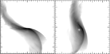
Figure 10: Broad-band $0.5-2.5$ keV intensity images from model cwb3. The left panel shows the emission at $i=0^{\circ}$. The right panel displays the emission at $i=30^{\circ}$ and $\phi=45^{\circ}$ (phase 0.875). The maximum intensity is $10^{7}\,{\rm erg\,cm^{-2}\,s^{-1}\,keV^{-1}\,ster^{-1}}$, and the major ticks on each axis mark out 0.5 mas. $\phi=0^{\circ}$ corresponds to the O8V star in front.

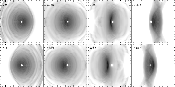
Figure 11: Broad-band $0.5-2.5$ keV intensity images from model cwb3 at $i=90^{\circ}$. From top to bottom and left to right the orbital phase is 0.0 ($\phi=0^{\circ}$, conjunction, O8V star in front), 0.125, 0.25 ($\phi=270^{\circ}$, quadrature), 0.375, 0.5 ($\phi=180^{\circ}$, conjunction, O6V star in front), 0.625, 0.75 ($\phi=90^{\circ}$, quadrature), and 0.875. The maximum intensity is $10^{7}\,{\rm erg\,cm^{-2}\,s^{-1}\,keV^{-1}\,ster^{-1}}$, and the major ticks on each axis mark out 0.5 mas.

3.3 Model cwb3

3.3.1 Images

The stellar winds in model cwb3 are of unequal strength, being blown from hypothetical O6V and O8V stars. The stronger wind from the O6V star pushes the WCR closer towards the O8V star, and, compared to model cwb2 where the winds are of equal strength, bends the arms of the WCR inwards towards the weaker wind. The left panel of Fig. 10 shows broad-band $0.5-2.5$ keV intensity images from model cwb3 for an observer directly above/below the orbital plane. A comparison against the corresponding image in Fig. 7 reveals several differences. Firstly, the brightest part of the image (at the apex of the WCR) is located closer to the O8V star (which is to the south in these images). Secondly, the downstream positions of the arms of the WCR are also in different locations, due to the different ram-pressure balance of the winds. Thirdly, there are differences in the brightness contrast across the contact discontinuity. At the apex of the WCR, ram pressure balance requirements mean that since the O8V wind has a lower pre-shock velocity than the O6V wind, the O8V material must have a higher pre-shock density. This directly translates into a higher post-shock density (and lower post-shock temperature), and thus into greater X-ray emissivity on the O8V side of the contact discontinuity. A similar effect is also seen from the thermal radio emission (see Paper II). This emission contrast is then amplified in the leading arm of the WCR, but reduced in the trailing arm, as a result of the dynamics of the WCR (see Paper I). In comparison, there is initially no contrast in the emission across the contact discontinuity at the apex of the WCR in model cwb2, though such an effect subsequently develops in the downstream arms. Finally, we note that due to velocity shear Kelvin-Helmholtz instabilities occur along the contact discontinuity in model cwb3, and these are also visible in the images. The clearest sign occurs at phases 0.375 and 0.875 in Fig. 11, where an oscillation of the contact discontinuity separating the bright and fainter parts of the WCR can be seen. The right panel in Fig. 7 shows the intensity image for an observer with $i=30^{\circ}$ and $\phi=45^{\circ}$. The O8V star is silhouetted against the WCR. The emission from the shocked O8V wind is clearly brighter, for the reasons already described above.

Fig. 11 shows broad-band $0.5-2.5$ keV intensity images from model cwb3 for an observer in the orbital plane with $\phi=0^{\circ}$ as a function of phase. The O8V star is in front at phase 0.0, while the larger O6V star is in front at phase 0.5. Significant differences to the images from model cwb2 are again apparent (cf. Fig. 8). For instance, at conjunction when the weaker O8V wind is in front (phase 0.0), the limb brightened edge of the leading arm of the WCR (to the right side of the image) shows greater curvature and is projected closer to the centre of the image, while the limb brightened part of the trailing arm is located at the far left side of the image. In addition, the O8V star occults a smaller region of the WCR than the larger O6V star does in model cwb2.

Other differences are also apparent. At phase 0.375, the double-helix-like structure seen from model cwb2 is replaced by a more imbalanced morphology, where the brightest regions trace the limb-brightened edge of the dense, shocked O8V gas on the trailing edge of the leading arm. Interestingly, compared to simulated radio images (see Fig. 12 in Paper II), at phase 0.875 the shocked O6V gas is much more visible on the right side of the image. Obviously the size of the occulted region differs depending on which star is in front, but we note that the position of this relative to the limb-brightened part of the WCR is also different at phase 0.375 and 0.875, reflecting the different amounts of downstream curvature imparted to the leading and trailing arms of the WCR (see Paper I for further details). Finally, we note that the vertical curvature of the WCR is also apparent in the images at quadrature (phase 0.25 and 0.75).

3.3.2 Lightcurves

The right column of Fig. 3 shows the orbital phase variation of the X-ray emission from model cwb3. The O8V star is in front at phase 0.0, with the O6V star in front at phase 0.5. The unequal wind strengths in model cwb3 is manifest in the unequal depths of the two minima around the orbit. The deeper minimum occurs when the O6V star (which has the denser wind) is in front of the WCR apex, as expected. A phase lead to the bottom of the minimum is present in some lightcurves (e.g. the $0.5-2.5$ keV curve), though not in others (e.g. the $2.5-10$ keV curve). The emisison at quadrature (phases 0.25 and 0.75) is brighter than at conjunction, as seen in the other simulations. The luminosity in the softest lightcurve is slightly higher near phase 0.25 than near 0.75. This is because lines of sight to the apex at phases near 0.25 initially pass through the hot, low opacity, gas in the WCR because of orbital aberration.

The X-ray luminosity is somewhat lower in this model compared to model cwb2, reflecting the reduced wind power of the O8V star. The reduction in luminosity is greatest in the harder energy bands (the $2.5-10$ keV luminosity in model cwb3 is only 40 per cent of the luminosity in model cwb2), reflecting the slower speed of the O8V wind and the increased obliquity of the shock in the primary wind with off-axis distance relative to model cwb2. The ISM corrected $0.5-10$ keV luminosity is $1.07\times 10^{33}\,\hbox{${\rm{\rm\thinspace erg}{\rm\thinspace s}^{-1}\,}$}$, $1.14\times 10^{33}\,\hbox{${\rm{\rm\thinspace erg}{\rm\thinspace s}^{-1}\,}$}$, and $1.16\times 10^{33}\,\hbox{${\rm{\rm\thinspace erg}{\rm\thinspace s}^{-1}\,}$}$ at viewing angles of $(i,\phi)=(90^{\circ},0^{\circ})$, $(90^{\circ},90^{\circ})$, and $(0,0)$ (pole-on). The slightly reduced X-ray luminosities compared to model cwb2 are somewhat offset by a corresponding reduction in $L_{\rm bol}$, giving $L_{\rm x}/L_{\rm bol}\approx 10^{-6}$ for all 3 of the viewing angles indicated, again consistent with strong colliding winds emission.

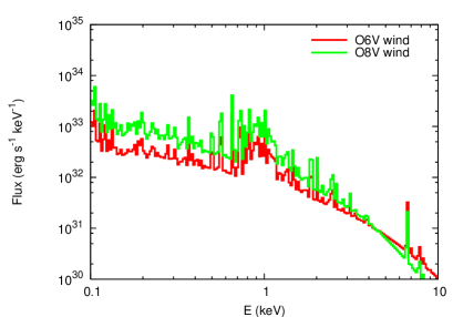
Figure 12: Intrinsic X-ray spectra from each shocked wind in model cwb3.

3.3.3 Spectra

The right column of Fig. 4 shows intrinsic and attenuated spectra from model cwb3. Because of the unequal winds, the emission at phases 0.5 (0.75) is no longer identical to that at phases 0.0 (0.25), so all conjunction and quadrature phases are shown. There is now a clear difference in the strength of the low energy absorption at orbital phases 0.0 and 0.5, reflecting changes to the wind density along sight lines when either the O8V or O6V stars are in front.

In models cwb1 and cwb2, the winds were of equal strength and the intrinsic emission from their shocked plasma was identical, and contributed equally to the total. However, Fig. 12 shows that the intrinsic emission from the postshock wind of the O6V star is harder than the intrinsic emission from the postshock wind of the O8V star. This reflects the higher velocity at which the O6V wind encounters the WCR, due to the greater distance over which it can accelerate and its higher terminal velocity (although this increase in the preshock velocity is somewhat offset by the greater shock obliquity further downstream). But while the shocked O6V wind dominates the hard emission, the shocked O8V wind dominates the overall intrinsic emission, as is clearly apparent in Fig. 12, contributing approximately two-thirds to the total luminosity. This is despite the total wind power of the O8V star being just one third of that of the O6V star. The fact that it dominates the X-ray luminosity is due to a greater fraction of it being processed through the WCR, and it subsequently radiating energy more efficiently (c.f. Pittard & Stevens 2002).

Figs. 5(e) and (f) show the “effective” circumstellar column and optical depth as a function of energy for various viewing angles into model cwb3. We find similar columns at phases 0.0 and 0.5 to those reported previously from models cwb1 and cwb2. The column at phase 0.5 (when the larger O6V star and its denser wind is in front) is slightly higher than at phase 0.0 (when the smaller O8V star is in front) as expected. The slope of the column with energy and its bin-to-bin variation are similar to those from model cwb2 shown in Fig. 5(c). As previously noted, the different wind strengths in model cwb3 break the symmetry that models cwb1 and cwb2 display at quadrature. Fig. 5(e) shows that the columns at phase 0.75 are very low at high energies, whereas they are significantly higher at phase 0.25. In contrast, the columns at $E<0.25$ keV at phase 0.0 and 0.75 are identical, whereas they are lower at phase 0.25.

The effective circumstellar column to an observer at $i=0^{\circ}$ is $1.7\times 10^{19}\;{\rm cm^{-2}}$ at 0.1 keV, rises an order of magnitude to $\approx 3\times 10^{20}\;{\rm cm^{-2}}$ by 1 keV, and then drops below $10^{19}\;{\rm cm^{-2}}$ by 7.5 keV. The $i=0^{\circ}$ circumstellar column and optical depth are greater than those from model cwb2, since the unequal wind strengths bend the WCR around the O8V star, so that only a relatively short segment along the line-of-sight from the apex of the WCR passes through hot plasma, with the rest of it through wind material from the O6V star.

3.3.4 Spectral fits

For model cwb3 we simulate Suzaku spectra with an exposure time of 20 ksec. Two-temperature mekal fits are poor ($\chi^{2}_{\nu}\approx 2.0$), and underestimate the hard X-ray flux. Three-temperature fits are much more acceptable (see Fig. 6(e) and (f), and Table 3). Significantly higher absorption is found to the hot component at phase 0.5 compared to phase 0.0, consistent with expectations given that the denser O6V wind is in front at phase 0.5. The temperature returned to the hottest mekal component is also significantly lower at phase 0.5 compared to phase 0.0. This reflects the much weaker Fe K line emission at phase 0.5, due to greater occultation (by a larger star) of the hottest part of the WCR at phase 0.5 (the surface brightness of the high energy emission falls off very rapidly from the apex of the WCR, and thus the observed flux of high energy X-rays is highly susceptible to the amount of occultation). No extra absorbing column (above the ISM value) is required to the separate mekal components in many of the fits. This is roughly consistent with Fig. 5(c) where it can be seen that the effective circumstellar column is typically low, due to the relatively small mass-loss rates and wide stellar separations in the model.

Having said this, significant additional absorption above the ISM value is returned from the fit made to the phase 0.5 spectrum. The degree of extra absorption increases with the temperature of the mekal component (no extra absorption is required to the lowest temperature mekal component in the fit). The additional absorption to the 0.85 keV component ($4^{+10}_{-4}\times 10^{20}\,{\rm cm^{-2}}$) is a bit lower than the effective circumstellar column at this energy in Fig. 5(e) (though within the 90 per cent confidence range the fitted value is reasonable). In contrast, the additional absorption to the 1.66 keV component ($3.6^{+1.2}_{-1.5}\times 10^{21}\,{\rm cm^{-2}}$) is both in better agreement with Fig. 5(e) and is more tightly constrained.

Interestingly, if the exposure time is reduced to 10 ksec, the fit to the $i=90^{\circ}$ phase 0.0 spectrum returns $kT_{3}=1.68^{+0.57}_{-0.16}$ keV. Although formally this is still consistent with the value returned from the fit to the 20 ksec exposure spectrum ($kT_{3}=2.09^{+0.12}_{-0.40}$ keV), it highlights that a lack of counts at high energies due to relatively short exposures can bias the resulting fits towards lower temperatures.

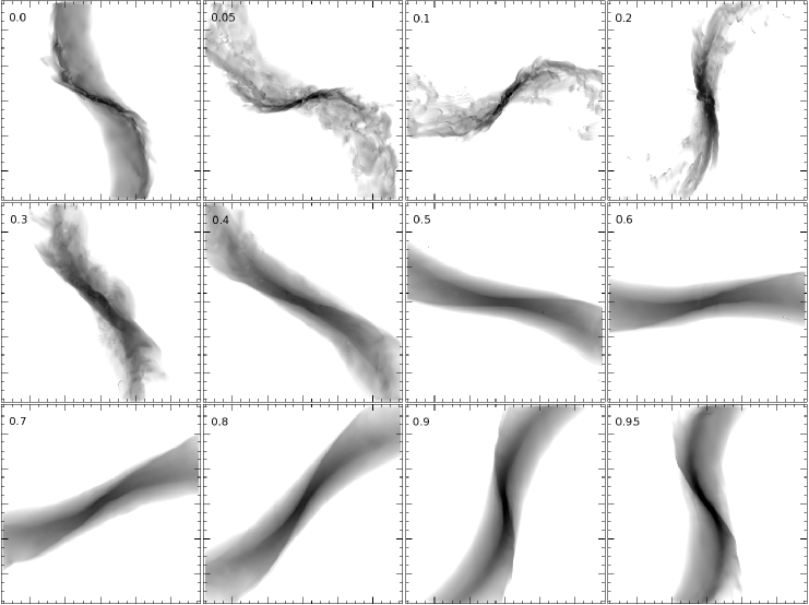
Figure 13: Broad-band ($0.5-2.5$ keV) intensity images from model cwb4 for an observer with $i=0^{\circ}$. The orbital phase is noted on each panel. The maximum intensity (black in the images) is $10^{8}\,{\rm erg\,cm^{-2}\,s^{-1}\,keV^{-1}\,ster^{-1}}$. The major ticks on each axis mark out 0.2 mas.

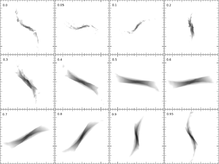
Figure 14: As Fig. 13 but showing broad-band ($2.5-10$ keV) intensity images. The grey scale and tick marks are the same as in Fig. 13.

3.4 Model cwb4

3.4.1 Images

In contrast to the previous models which all had circular orbits, model cwb4 simulates a CWB with an eccentric orbit ($e=0.36$). This introduces a time-dependence to the intrinsic emission, which now varies with phase, whereas it was constant in the circular orbit models cwb1$-$cwb3. Fig. 13 shows intensity images of the $0.5-2.5$ keV broad-band emission from model cwb4 for an observer directly above the orbital plane. The images show striking variations in their brightness and morphology as a function of orbital phase, reflecting the dramatic changes in the WCR during the orbit (see Paper I for full details of the hydrodynamics). Dramatic changes were also seen in the thermal radio-to-sub-mm emission (see Paper II for further details).

There is a smooth morphology to the emission from the WCR at phase 0.5 (apastron), when the WCR is adiabatic and instabilities are rare. As the stars progress in phase the WCR rotates in the images. The WCR becomes brighter and shows increasing curvature as the snapshots move towards the time of periastron passage (the maximum surface brightness of $1.9\times 10^{8}\,{\rm erg\,cm^{-2}\,s^{-1}\,keV^{-1}\,ster^{-1}}$ occurs at phase 0.95. At periastron there is a distinct change in the morphology of the images, with instabilities now clearly visible. This reflects the sudden cooling and formation of dense clumps within the WCR (see Paper I for further details). This morphology persists until phase 0.2, at which point the ratio of the cooling time to the flow time of the shocked gas near the apex of the WCR becomes significant again. Dense cold clumps which formed during the periastron passage are still present in the WCR, but there is now also a substantial volume of hot gas. These cold clumps are gradually destroyed or cleared out of the system, so that by phase 0.7 there is no longer any cold, post-shock, gas on the hydrodynamical grid (note, however, that even at phase 0.5 this process is far from complete). Careful examination reveals that individual clumps and their ablated tails are visible in these images, although the level of detail is not great enough for this to be apparent in Fig. 13. Since the WCR rotates to follow the motion of the stars, while the dense clumps flow out on almost ballistic trajectories, the clumps are often seen exiting the WCR through its trailing shock. They are then exposed to the full “fury” of whichever high-speed wind they find themselves in, and are enveloped by a bowshock and high temperature plasma. In Paper I it was speculated that this additional contribution to the overall amount of hot plasma in the system may be significant in terms of the resulting X-ray luminosity. However, it is now clear from Fig. 13 that such regions have a negligible effect in this regard (although careful inspection reveals that there are in fact noticeable features in the intensity images).

Fig. 14 shows intensity images of the $2.5-10$ keV emission. The emission is clearly less extended and is more concentrated towards the central part of the WCR. Otherwise the morphology and brightness of the emission behaves in a rather similar way to that in the $0.5-2.5$ keV images. The highest surface brightness of $3.5\times 10^{7}\,{\rm erg\,cm^{-2}\,s^{-1}\,keV^{-1}\,ster^{-1}}$ occurs at phase 0.9.

3.4.2 Lightcurves and spectra

Fig. 15 displays the lightcurves which are obtained from model cwb4. The top panels show lightcurves of the intrinsic emission (red curves), while the bottom panels show attenuated lightcurves. The intrinsic X-ray emission is no longer constant with phase, but, at low energies, reaches a maximum at or near periastron as the stars reach their point of closest approach (Fig. 15a). In contrast the $2.5-10$ keV intrinsic emission (Fig. 15e) peaks at phase 0.9, and then undergoes a precipitous drop so that it is actually close to its minimum value at periastron.

The phase-dependence of the intrinsic emission is complicated, and depends on a combination of factors, including the current separation of the stars, their separation in the recent past, and the variation of the pre-shock wind densities and speeds and the post-shock cooling efficiency over this interval. The intrinsic emission from systems where the WCR is largely adiabatic should scale as $1/d_{\rm sep}$ (Stevens et al. 1992). This relationship breaks if cooling within the WCR becomes important (cf. Fig. 9 in Pittard & Stevens 1997), and/or if the pre-shock speeds of the winds change. Both of these events occur in model cwb4, so therefore it is not surprising that the intrinsic luminosity does not follow this scaling. In fact the intrinsic luminosity varies by factors of approximately 20, 4 and 20 in the $0.1-0.5$, $0.5-2.5$ and $2.5-10$ keV lightcurves, respectively, whereas for comparison a $1/d_{\rm sep}$ response predicts only a factor of 2 variation. For an observer with viewing angles of $i=90^{\circ}$ and $\phi=0^{\circ}$, the ISM corrected $0.5-10$ keV luminosity varies between $1.22\times 10^{33}\,\hbox{${\rm{\rm\thinspace erg}{\rm\thinspace s}^{-1}\,}$}$ at phase 0.1, and $4.53\times 10^{33}\,\hbox{${\rm{\rm\thinspace erg}{\rm\thinspace s}^{-1}\,}$}$ at phase 0.95, representing a change in $L_{\rm x}/L_{\rm bol}$ from $8.56\times 10^{-7}$ to $3.18\times 10^{-6}$, respectively. For an observer located pole-on ($i,\phi=0^{\circ},0^{\circ}$), $L_{\rm x}/L_{\rm bol}$ varies between $7.01\times 10^{-7}$ at phase 0.1 to $5.88\times 10^{-6}$ at phase 0.95. The peak values of $L_{\rm x}/L_{\rm bol}$ are the highest obtained from any of the models in this work, and indicate not only the strength of the colliding winds emission in this system, but also the relative ease with which the X-ray photons escape the system at favourable orientations because of the nature of the WCR.

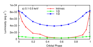
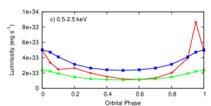
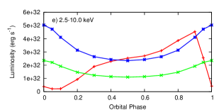
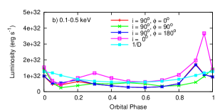
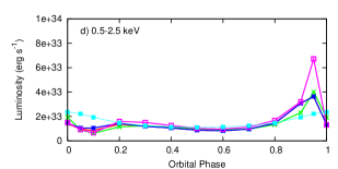
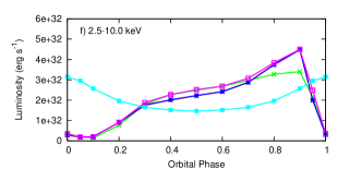
Figure 15: X-ray lightcurves for model cwb4. The lightcurves were calculated over the energy bands $0.1-0.5\;$keV (left), $0.5-2.5\;$keV (middle), and $2.5-10\;$keV (right). The top panels show the intrinsic luminosity (red curves), while the bottom panels show the attenuated (observed) luminosity for viewing angles in the orbital plane ($i=90^{\circ}$) with $\phi=0^{\circ}$, $90^{\circ}$, and $180^{\circ}$ (red, green and blue curves, respectively), and directly above/below the orbital plane ($i=0^{\circ}$, pink curves). In all panels curves displaying a $1/d_{\rm sep}$ variation (with arbitrary normalization) are over-plotted.

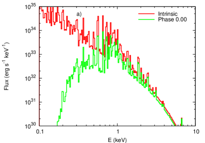
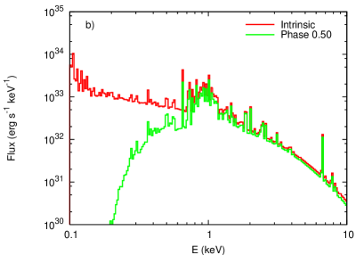
Figure 16: Intrinsic and attenuated X-ray spectra from model cwb4 for viewing angles $i=90^{\circ}$ and $\phi=0^{\circ}$ at a) periastron, and b) apastron.

To understand the behaviour of the intrinsic lightcurves of model cwb4, one needs to examine the intrinsic spectra, which display strong phase-locked variation. Fig. 16 shows that the spectral hardness of the intrinsic X-ray emission changes by a huge amount between periastron and apastron. At periastron the emission is very soft, reflecting the low pre-shock wind speeds at this phase ($710\hbox{${\rm{\rm\thinspace km}{\rm\thinspace s}^{-1}\,}$}$ along the line of centres), whereas the emission is much harder at apastron, since the increase in the stellar separation allows the winds to accelerate to higher speeds before their collision ($1665\hbox{${\rm{\rm\thinspace km}{\rm\thinspace s}^{-1}\,}$}$ along the line of centres), and reduces the effects of radiative inhibition (see Paper I).

Interestingly, the intrinsic X-ray spectrum is at its hardest at phase 0.6, rather than at apastron. Thereafter, the intrinsic emission begins to soften as the stars move closer together, the preshock wind speeds decline, and the WCR becomes increasingly radiative (see Fig. 17b). The softening is initially manifest as an increase in the soft emission, while the harder emission (e.g. $E>4\;$keV) remains at a relatively constant flux until phase 0.9. Up to this point the flux at high energies appears to be finely balanced between the intrinsic softening of the spectrum and the increasing luminosity as the stars approach each other. However, this balancing act is over by phase 0.9, after which the spectral softening rapidly accelerates. Between phase 0.9 and 1.0 (periastron) there is a precipitous collapse in the hard X-ray emission, as the stars move deep within the acceleration zone of the other’s wind. The intrinsic emission is of comparable softness at phase 1.0 and 1.1 (but brighter at phase 1.0 due to the reduced stellar separation), and is markedly harder by phase 0.2 (see Fig. 17a). These variations in the intrinsic spectra explain the intrinsic lightcurves shown in the top panels of Fig. 15.

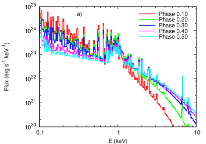
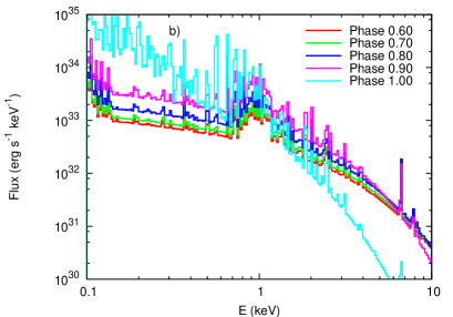
Figure 17: Intrinsic X-ray spectra from model cwb4 as a function of orbital phase. a) Phase $0.1-0.5$. b) Phase $0.6-1.0$.

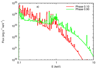
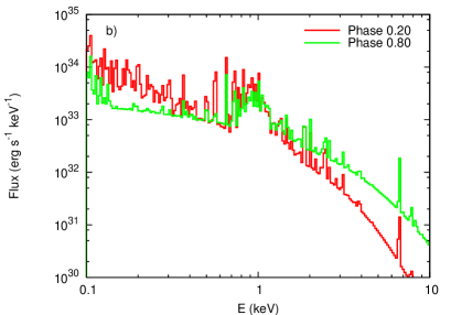
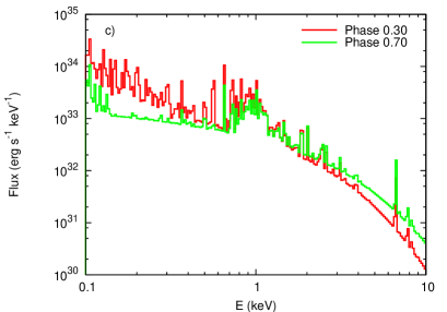
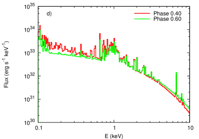
Figure 18: Intrinsic X-ray spectra from model cwb4 as a function of orbital phase. In each panel the stars are at identical separations, and either receding (phase $<0.5$) or approaching (phase $>0.5$). The hysteresis of the spectra is clearly evident.

Fig. 18 reveals that there is a strong hysteresis to the intrinsic emission, with large differences in the spectrum at identical stellar separations depending on whether the stars are approaching or receding from each other. The emission is much harder as the stars move together compared to when they separate: this is a natural consequence of the higher pre-shock wind speeds that are attained prior to reductions in the stellar separation. As the stars approach each other the conditions in the WCR reflect, to some extent, the hot and rarefied plasma created at earlier orbital phases. Similarly, as the stars recede the downstream conditions in the WCR reflect still the lower preshock velocities at earlier orbital phases, and in extremum the cold, dense plasma created during periastron passage. The hysteresis is largest nearest periastron, when changes in the pre-shock conditions are at their most rapid, and smallest near apastron when the rate of change in the stellar separation is most sedate. The observed hysteresis is also partly due to variations in the relative wind speeds towards each star - when the stellar separation is decreasing, the stars (and thus also their winds) have a component of their orbital velocity directed towards each other, which augments the wind speeds in the centre of mass frame. The opposite effect occurs when the stars recede from each other. This mechanism enhances the post-shock temperature in the WCR after apastron, and reduces it at comparable orbital phases prior to apastron. Hysteresis of the thermal radio and sub-mm emission also occurs (see Paper II).

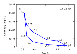
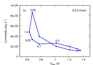
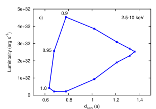
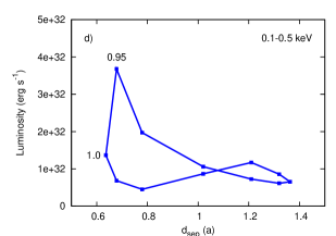
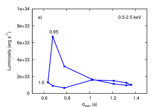
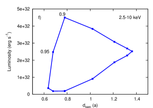
Figure 19: Intrinsic (top row) and attenuated (bottom row) X-ray luminosities from model cwb4 as a function of orbital separation. The energy bands $0.1-0.5$ keV (left), $0.5-2.5$ keV (middle), and $2.5-10$ keV (right), are shown. The attenuated lightcurves are for an observer located directly above the orbital plane ($i=0^{\circ}$). Some orbital phases are marked on the plots.

The hysteresis of the intrinsic emission is also clear when the luminosities are plotted against stellar separation, as shown in Fig. 19(a)-(c). Interestingly, the intrinsic emission in the $2.5-10$ keV band is stronger as the stars approach periastron, whereas the emission in the $0.1-0.5$ keV band is stronger as the stars recede. The hard emission requires high temperature plasma, which the WCR is full of in the second half of the orbit, but which is comparatively lacking in the first half of the orbit. In contrast, emission in the soft band does not require such high temperatures. Instead it is strongest when the postshock densities are high, such as during the formation of cold clumps within the WCR. Some of this emission will be from intermediate temperature interface regions where hot plasma surrounds cooler clumps. In comparison the intrinsic emission in the $0.5-2.5$ keV band displays a transitional state: the emission is brighter in some parts of the orbit when the stars are receding, and fainter in other parts.

Armed with an understanding of how the intrinsic X-ray emission varies with orbital phase, we now examine the attenuated emission. The attenuated lightcurves shown in the bottom panels of Fig. 15 display behaviour which depends on the viewing angle of the observer. The lightcurves for observers at $i=90^{\circ}$ and $\phi=0$ or $180^{\circ}$ are almost identical, particularly in the hard $2.5-10$ keV band. Such symmetry is expected, given the identical stellar parameters. The $2.5-10$ keV attenuated lightcurves show the closest behaviour to their intrinsic counterpart, highlighting the ability of hard X-rays to stream through the circumstellar environment relatively unaffected by absorption. For this same reason the $2.5-10$ keV attenuated lightcurves also show very little change with the viewing angle of the observer, with the largest difference occuring at phases $0.8-0.9$ when there is more attenuation for an observer at $i=90^{\circ}$ and $\phi=90^{\circ}$ than for other orientations, because the stars are eclipsing the apex of the WCR at this time (see Paper I).

The attenuated $0.5-2.5$ keV lightcurves all peak at phase 0.95, irrespective of the orientation of the observer, in agreement with the timing of the peak in the intrinsic lightcurve. However, the height and shape of the maximum in the attenuated lightcurves is dependent on the orientation. The greatest luminosity in the attenuated $0.5-2.5$ keV lightcurves occurs for an observer viewing the system face on ($i=0^{\circ}$). In contrast, the timing of the maximum in the attenuated $0.1-0.5$ keV lightcurves is strongly dependent on the viewer’s orientation, ranging from phase 0.9 for observers in the orbital plane at viewing angles of $\phi=0^{\circ}$ and $180^{\circ}$, to phase 0.0 (periastron) for a viewing angle of $\phi=90^{\circ}$. For an observer viewing the system face on the maximum occurs at phase 0.95 - incidentally, this is also the highest maximum seen in the $0.1-0.5$ keV lightcurves. These differences in the timing of the maxima reflect the propensity for soft X-rays to be attenuated by the circumstellar environment, and the dependence of the strength of this attenuation on the orientation of the observer. The strong circumstellar absorption near periastron arises from the enhanced wind densities around the WCR due to the reduced stellar separation and pre-shock wind speeds.

Broad minima which are roughly centered on apastron occur in most of the attenuated $0.1-0.5$ keV and $0.5-2.5$ keV lightcurves, though there is a slight maximum at apastron in the $0.1-0.5$ keV lightcurve for an observer with $i=90^{\circ}$ and $\phi=90^{\circ}$ (since lines-of-sight from the apex of the WCR initially pass through the low opacity WCR). The minima following periastron are generally deepest at phase 0.1. The shape of the minimum is also generally quite smooth, though the $0.1-0.5$ keV lightcurves for $i=90^{\circ}$ and $\phi=0^{\circ}$ and $180^{\circ}$ are noticeable for showing more structure (Fig. 15(b) shows the luminosity levelling out between phases $0.95-1.0$, before falling more steeply between phases $0.0-0.05$).

Panels (d)-(f) of Fig. 19 show the attenuated luminosities in the three energy bands for an observer at $i=90^{\circ}$ as a function of orbital separation. The $2.5-10$ keV emission is most similar to its intrinsic counterpart (Fig. 19c), again illustrating the relative ease at which the hard X-rays travel through the circumstellar environment. In contrast, the emission in the $0.1-0.5$ keV band suffers severe attenuation, and this has a large impact on the shape of its hysteresis curve (compare Figs. 19a and d). As we have already seen, the attenuation is particularly severe after periastron, when there is not much hot, low opacity, plasma in the WCR.

The eccentric orbit means that the emission from model cwb4 at various times resembles that from models cwb1 and cwb2. Careful examination reveals that the periastron spectrum (Fig. 16a) is slightly harder than the phase 0.0 spectrum from model cwb1 (cf. Fig. 4a), with the Fe K emission visible in the former plot. This reflects the fact that the downstream flow in model cwb4 contains hotter plasma (which was shocked when the winds previously collided at a higher speed) than in model cwb1. That they are otherwise so similar reflects the fact that emission at the apex of the WCR (which responds much quicker to changing pre-shock conditions than emission from far downstream) dominates the total emission in this model as the post-shock gas at the apex of the WCR rapidly becomes extremely radiative.

Likewise, there is a high degree of similarity between the apastron spectrum (Fig. 16b) and the phase 0.5 spectrum from model cwb2 (cf. Fig. 4c), the former being slightly softer. This is again consistent with the recent history of the WCR. Their likeness reflects the fact that in model cwb4, the rate of change in the stellar separation is at its most sedate at apastron. The dynamical timescale for flow out of the system is then short compared to the timescale for significant orbital change. At phase 0.5, $t_{\rm flow}\sim\frac{d_{\rm sep}}{v_{\infty}/2}\approx 0.5\;$d, while the time for the orbital separation to change 10 per cent from its apastron value is $0.19\;P_{\rm orb}=1.2\;$d.

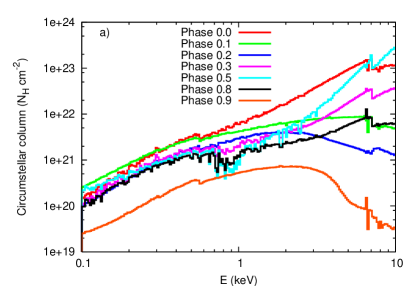
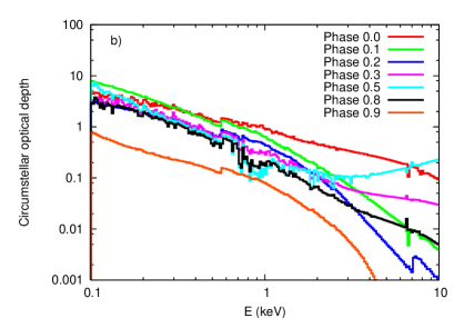
Figure 20: a) “Effective” circumstellar column (a) and optical depth (b) from model cwb4 for an observer in the orbital plane ($i=90^{\circ}$) as a function of energy and orbital phase. Note that occultation can severely affect the value of the “effective” column. It is therefore not always an accurate reflection of the column that the observed X-rays pass through (see Sec. 3.1.3 for further details).

Fig. 20 shows the effective circumstellar column and optical depth as a function of energy and orbital phase for an observer with $i=90^{\circ}$ and $\phi=0^{\circ}$. The columns at phase 0.0 and 0.5 bear some similarity to those obtained from models cwb1 and cwb2, in the same way that the attenuated spectra do. Thus, to first order there is rough agreement between the emission and absorption characteristics of an eccentric system at periastron and apastron and circular systems of identical stellar separation, at least for the region of parameter space covered in these models.

Fig. 20(a) also shows that there are extremely large phase-dependent variations in the energy-dependent column. The variation of the column to the high energy (e.g. 5 keV) emission is largely due to changes in the degree of occultation to this emission, with high occultation at conjunction (phase 0.0 and 0.5), and lesser occultation near quadrature (phase 0.14 and 0.86). There is a severe decline in the column to the high energy emission (due largely to changes in the degree of occultation) between periastron and phase 0.1. At phase 0.2 the observer views the WCR apex through hot plasma further downstream (see Fig. 10 in Paper I), and the circumstellar column declines at all energies. By phase 0.3 one of the stars is already positioning itself in front of parts of the apex of the WCR, and the column to the high energy emission increases from its value at phase 0.2. The high energy column further increases to a maximum near phase 0.5. The column to the high energy emission eases again by phase 0.8, while at phase 0.9 the observer again views the WCR apex through hot plasma further downstream, which results in the lowest effective column and optical depth at all energies and phases.

In contrast to the 4 orders of magnitude variation in the column at 10 keV, the column to the low energy emission is surprisingly steady during the majority of the orbit, which reflects the large volume from which this emission arises. However, there is again a significant reduction in the low energy circumstellar column at phase 0.9 due to the reasons previously given.

The phase dependent variation in the optical depth shown in Fig. 20(b) to a large part reflects the changes in the circumstellar columns commented on above. The variation in the optical depth as a function of phase spans the range $0.8-7$ at 0.1 keV, $0.1-1$ at 1 keV, and $<10^{-3}-0.2$ at 10 keV.

3.4.3 Spectral fits

Table 5 and Fig. 21 show the results of spectral fits to “fake” Suzaku spectra with a nominal exposure time of 20 ksec generated from model cwb4. The spectra in Fig. 21 were specifically chosen to highlight the large spectral variations which occur over the course of the stellar orbit. The spectrum at phase 0.0 is almost as soft as the emission gets in this model (the spectrum at phase 0.05 is marginally softer), reflecting the strong cooling of the plasma in the WCR at this phase. By phase 0.2 (not shown) the spectrum is noticeably harder (and more luminous). The spectrum at phase 0.6 is about as hard as the emission gets, and shows a prominent Fe K line. At phase 0.95 the spectrum is at its most luminous, and is again softer, reflecting the lower pre-shock wind speeds at this phase. There are now not enough counts at high energies to detect the Fe K line in the binned spectra, though it is of course seen in our theoretical spectra.

The spectral variability shown in Fig. 21 is reflected in changes in the values of the fit parameters (see Table 5), which are plotted in Fig. 22. The temperature of the hottest mekal component shows significant variation, changing from $0.66^{+0.11}_{-0.03}$ keV at phase 0.05, to $2.53^{+0.25}_{-0.17}$ keV at phase 0.7. In addition, significant enhancements in the normalization of the components occur as periastron is approached. Between apastron and phase 0.95 the normalization of the hot component increases by a factor of 4.6, far above the corresponding $1/d_{\rm sep}$ value. Panel d) shows the combined luminosity of the three mekal components. A comparison with Fig. 15 reveals that the fits do a good job of recovering the phase variation of the observed and also the intrinsic luminosity. It is clear that the fits infer the presence of significant circumstellar absorption between phases $0.95-1.05$, which is responsible for the large difference in the intrinsic and ISM corrected luminosities.

It is also noteable that the normalization of the hot component dominates those of the cooler components from phase 0.4 to 0.95, while the normalization to the warm (i.e. the second) component dominates at phase 0.0 and 0.05. There is no need for additional circumstellar absorption to the mekal components at phase 0.9, which is consistent with the low value of the effective circumstellar column at this phase (see Fig. 20a). While the fits do require substantial additional column to the warm component at phase 0.0 ($1.13^{+0.23}_{-0.21}\times 10^{22}\,{\rm cm^{-2}}$), this extra absorption is about 3 times higher than the effective circumstellar column at 0.49 keV, as shown in Fig. 20a). It is also puzzling why the spectral fitting did not require extra absorption (above the ISM value) to the cold and hot mekal components at this phase, despite these making significant contributions to the overall observed emission (see the top left panel in Fig. 21).

Figure 21: Three-temperature fits to “fake” Suzaku spectra from model cwb4 for an observer in the orbital plane viewing the system at conjunction ($\phi=0^{\circ}$). a) Phase 0.0, b) phase 0.6, c) phase 0.95. The dramatic variation of the spectra with orbital phase is clearly shown. The assumed exposure time is 20 ksec in each case.

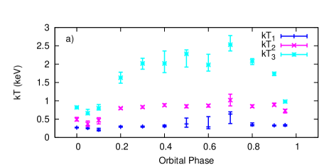
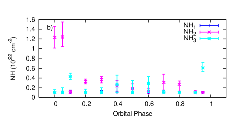
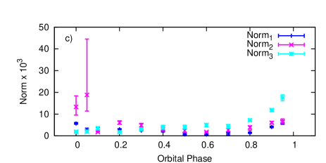
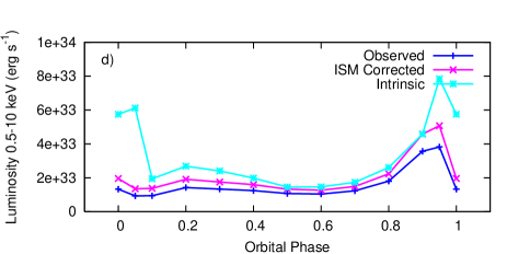
Figure 22: Orbital phase variability of the fit parameters to the “fake” Suzaku spectra from model cwb4 for an observer with $i=90^{\circ}$ and $\phi=0^{\circ}$. Panel a) shows the temperature variation, panel b) the variation in the absorbing column (the displayed values include the assumed ISM column of $N_{\rm H}=10^{21}\,{\rm cm^{-2}}$), and panel c) the variation of the normalization, of each fit component. Panel d) shows the observed, ISM corrected and intrinsic luminosity of each component combined.

Table 3: Spectral fitting results to simulated spectra from models cwb1, cwb2, and cwb3. The normalization of the mekal components (norm) is defined as $[10^{-14}/(4\pi D^{2})]\int n_{\rm e}\,n_{\rm H}\,dV$, where $D$ is the distance to the source (in cm), and $n_{\rm e}$ and $n_{\rm H}$ are the electron and hydrogen number densities (in ${\rm cm^{-3}}$), respectively. The indicated range in each fit parameter is the 90 per cent confidence interval for one interesting parameter. The last three columns give the observed flux, the flux corrected for ISM absorption, and the intrinsic flux, between 0.5 and 10 keV. All fits are to “fake” observations of 10 ksec duration, except the Suzaku observations of models cwb2 and cwb3, where the assumed exposure times are 40 ksec and 20 ksec, respectively.

Model	Phase	Model fit	$kT$	$N_{\rm H}$	Norm	$\chi^{2}_{\nu}$ (d.o.f.)	Observed flux	ISM corrected flux	Intrinsic flux
			(keV)	($10^{22}\,{\rm cm^{-2}}$)	($10^{-3}$)		(${\rm 10^{-12}erg\,cm^{-2}\,s^{-1}}$)
Chandra fits
cwb1	0.0	2T	$0.28^{0.31}_{0.25}$	$0.1^{0.18}_{0.1}$	$2.02^{3.45}_{1.90}$	1.27 (93)	$2.27$	$3.70$	$37.0$
			$0.65^{0.80}_{0.61}$	$0.59^{0.67}_{0.52}$	$4.07^{4.58}_{2.86}$		$2.21$	$2.74$	$10.4$
cwb1	0.25	2T	$0.25^{0.27}_{0.24}$	$0.1^{0.13}_{0.1}$	$4.19^{5.27}_{3.98}$	1.71 (110)	$4.21$	$71.3$	$71.3$
			$0.67^{0.70}_{0.64}$	$0.39^{0.42}_{0.35}$	$6.09^{6.32}_{5.62}$		$5.31$	$6.81$	$15.5$
cwb2	0.0	3T	$0.33^{0.36}_{0.31}$	$0.1^{0.15}_{0.1}$	$2.69^{3.66}_{2.26}$	1.13 (165)	$3.51$	$5.46$	$5.46$
			$1.01^{1.05}_{0.94}$	$0.25^{0.34}_{0.1}$	$3.45^{4.55}_{2.15}$		$4.01$	$4.90$	$6.99$
			$2.47^{3.25}_{2.03}$	$0.31^{0.56}_{0.1}$	$3.58^{4.81}_{2.55}$		$3.68$	$4.00$	$5.14$
cwb2	0.25	3T	$0.32^{0.34}_{0.26}$	$0.10^{0.32}_{0.1}$	$2.18^{5.67}_{1.92}$	1.04 (171)	$2.75$	$4.31$	$4.34$
			$0.84^{0.93}_{0.78}$	$0.1^{0.24}_{0.1}$	$1.63^{2.45}_{1.44}$		$2.86$	$3.75$	$3.75$
			$2.02^{2.12}_{1.92}$	$0.1^{0.15}_{0.1}$	$5.55^{5.84}_{5.09}$		$6.65$	$7.76$	$7.76$
Suzaku fits
cwb1	0.0	3T	$0.11^{0.14}_{0.0}$	$0.17^{0.36}_{0.1}$	$4.21^{69.6}_{0.84}$	1.50 (324)	$0.30$	$0.64$	$1.08$
			$0.31^{0.33}_{0.29}$	$0.15^{0.23}_{0.1}$	$2.17^{3.63}_{1.57}$		$2.19$	$3.40$	$4.24$
			$0.69^{0.74}_{0.66}$	$0.57^{0.62}_{0.53}$	$3.34^{3.65}_{2.78}$		$1.99$	$2.45$	$8.46$
cwb1	0.25	3T	$0.12^{0.14}_{0.14}$	$0.102^{0.21}_{0.1}$	$3.17^{7.11}_{0.0}$	2.28 (401)	$0.58$	$1.26$	$1.28$
			$0.31^{0.31}_{0.30}$	$0.14^{0.14}_{0.1}$	$4.64^{5.47}_{3.80}$		$4.85$	$7.57$	$9.03$
			$0.74^{0.74}_{0.73}$	$0.41^{0.43}_{0.40}$	$4.60^{4.80}_{4.38}$		$3.91$	$4.89$	$11.4$
cwb2	0.0	3T	$0.33^{0.35}_{0.31}$	$0.1^{0.14}_{0.1}$	$1.89^{2.43}_{1.59}$	1.18 (295)	$2.46$	$3.82$	$3.82$
			$0.88^{0.94}_{0.85}$	$0.17^{0.28}_{0.1}$	$2.23^{3.04}_{1.74}$		$3.26$	$4.16$	$4.96$
			$2.38^{2.55}_{2.10}$	$0.1^{0.27}_{0.1}$	$4.10^{4.86}_{3.69}$		$5.08$	$5.84$	$5.84$
cwb2	0.25	3T	$0.31^{0.33}_{0.29}$	$0.1^{0.13}_{0.1}$	$2.17^{2.81}_{1.91}$	1.17 (319)	$2.70$	$4.26$	$4.26$
			$0.83^{0.87}_{0.79}$	$0.13^{0.31}_{0.1}$	$1.91^{3.15}_{1.63}$		$3.15$	$4.10$	$4.41$
			$2.14^{2.26}_{2.02}$	$0.1^{0.17}_{0.1}$	$5.16^{5.56}_{4.60}$		$6.24$	$7.25$	$7.25$
cwb3	0.0	3T	$0.30^{0.31}_{0.29}$	$0.1^{0.12}_{0.1}$	$1.82^{2.05}_{1.61}$	1.21 (339)	$2.20$	$3.50$	$3.50$
			$0.84^{0.87}_{0.82}$	$0.15^{0.24}_{0.1}$	$1.71^{2.21}_{1.43}$		$2.65$	$3.43$	$3.93$
			$2.09^{2.21}_{1.69}$	$0.1^{0.41}_{0.1}$	$2.12^{2.86}_{1.90}$		$2.55$	$2.97$	$2.97$
cwb3	0.25	3T	$0.30^{0.31}_{0.28}$	$0.1^{0.11}_{0.1}$	$1.69^{1.87}_{1.54}$	1.35 (353)	$2.02$	$3.23$	$3.23$
			$0.85^{0.88}_{0.81}$	$0.10^{0.18}_{0.1}$	$1.50^{1.85}_{1.37}$		$2.62$	$3.43$	$3.23$
			$1.79^{1.89}_{1.71}$	$0.1^{0.12}_{0.1}$	$2.60^{2.77}_{2.47}$		$3.08$	$3.63$	$3.63$
cwb3	0.5	3T	$0.29^{0.31}_{0.28}$	$0.1^{0.12}_{0.1}$	$1.75^{1.97}_{1.57}$	1.14 (324)	$2.05$	$3.30$	$3.30$
			$0.85^{0.88}_{0.83}$	$0.14^{0.24}_{0.1}$	$1.57^{2.09}_{1.32}$		$2.48$	$3.21$	$3.60$
			$1.66^{1.86}_{1.54}$	$0.46^{0.58}_{0.31}$	$2.67^{3.07}_{2.16}$		$2.14$	$2.35$	$3.84$
cwb3	0.75	3T	$0.30^{0.31}_{0.29}$	$0.1^{0.12}_{0.1}$	$1.75^{2.01}_{1.63}$	0.94 (356)	$2.12$	$3.38$	$3.38$
			$0.85^{0.88}_{0.83}$	$0.1^{0.14}_{0.1}$	$1.66^{1.83}_{1.55}$		$2.89$	$3.78$	$3.78$
			$1.99^{2.08}_{1.90}$	$0.1^{0.12}_{0.1}$	$2.51^{2.66}_{2.40}$		$3.02$	$3.52$	$3.52$

Table 4: Comparison of the intrinsic $0.5-10$ keV luminosity of the theoretical spectra with that obtained from the spectral fits. All values are in units of $10^{33}\hbox{${\rm{\rm\thinspace erg}{\rm\thinspace s}^{-1}\,}$}$. The percentage ratio of the inferred to the actual intrinsic luminosity is shown in brackets for each case.

	Model cwb1	Model cwb2
Intrinsic luminosity	$3.11$	$1.81$
Chandra phase 0.0	$1.69$ (54%)	$2.10$ (116%)
Chandra phase 0.25	$2.71$ (87%)	$1.90$ (105%)
Suzaku phase 0.0	$1.65$ (53%)	$1.75$ (97%)
Suzaku phase 0.25	$2.59$ (83%)	$1.90$ (105%)

Table 5: As Table 3 but for model cwb4. All the fits are of 3-temperature mekal models to simulated Suzaku spectra of 20 ksec duration, for an assumed inclination $i=90^{\circ}$.

Phase	$kT$	$N_{\rm H}$	Norm	$\chi^{2}_{\nu}$ (d.o.f.)	Observed flux	ISM corrected flux	Intrinsic flux
	(keV)	($10^{22}\,{\rm cm^{-2}}$)	($10^{-3}$)		(${\rm 10^{-12}erg\,cm^{-2}\,s^{-1}}$)
0.00	$0.27^{0.28}_{0.26}$	$0.1^{0.11}_{0.1}$	$5.65^{6.13}_{5.35}$	1.51 (253)	$6.04$	$10.0$	$10.0$
	$0.49^{0.55}_{0.45}$	$1.23^{1.46}_{1.01}$	$13.3^{18.4}_{9.52}$		$1.72$	$1.99$	$33.7$
	$0.82^{0.85}_{0.79}$	$0.1^{0.16}_{0.1}$	$1.88^{2.25}_{1.62}$		$3.33$	$4.38$	$4.38$
0.05	$0.26^{0.31}_{0.24}$	$0.1^{0.13}_{0.1}$	$2.81^{3.53}_{2.49}$	1.41 (218)	$2.94$	$4.91$	$4.91$
	$0.37^{0.45}_{0.30}$	$1.24^{1.55}_{1.04}$	$18.8^{44.5}_{11.4}$		$1.39$	$1.64$	$41.5$
	$0.66^{0.77}_{0.63}$	$0.1^{0.20}_{0.1}$	$1.86^{2.59}_{1.59}$		$3.48$	$4.76$	$4.76$
0.10	$0.21^{0.25}_{0.18}$	$0.1^{0.15}_{0.1}$	$2.35^{3.75}_{2.02}$	1.32 (209)	$1.91$	$3.48$	$3.48$
	$0.47^{0.54}_{0.37}$	$0.1^{0.14}_{0.1}$	$1.78^{2.17}_{1.36}$		$3.07$	$4.44$	$4.44$
	$0.80^{0.90}_{0.75}$	$0.43^{0.50}_{0.37}$	$3.50^{4.17}_{2.68}$		$2.90$	$3.57$	$8.30$
0.20	$0.29^{0.28}_{0.31}$	$0.1^{0.11}_{0.1}$	$2.97^{3.29}_{2.75}$	1.35 (290)	$3.51$	$5.62$	$5.62$
	$0.80^{0.82}_{0.77}$	$0.33^{0.38}_{0.28}$	$6.03^{6.92}_{5.33}$		$6.23$	$7.83$	$14.3$
	$1.63^{1.78}_{1.48}$	$0.1^{0.17}_{0.1}$	$1.75^{2.11}_{1.41}$		$2.13$	$2.53$	$2.53$
0.30	$0.30^{0.31}_{0.28}$	$0.1^{0.14}_{0.1}$	$2.45^{2.91}_{2.23}$	1.12 (298)	$2.94$	$4.69$	$4.69$
	$0.83^{0.86}_{0.80}$	$0.37^{0.43}_{0.30}$	$4.84^{5.75}_{4.02}$		$4.59$	$5.68$	$11.2$
	$2.02^{2.16}_{1.86}$	$0.1^{0.20}_{0.1}$	$3.03^{3.49}_{2.86}$		$3.64$	$4.24$	$4.24$
0.40	$0.31^{0.34}_{0.29}$	$0.1^{0.13}_{0.1}$	$2.10^{2.54}_{1.75}$	1.05 (287)	$2.61$	$4.12$	$4.12$
	$0.88^{0.92}_{0.85}$	$0.24^{0.35}_{0.11}$	$3.11^{4.12}_{2.24}$		$3.91$	$4.92$	$6.96$
	$2.02^{2.36}_{1.77}$	$0.27^{0.46}_{0.1}$	$3.92^{4.86}_{3.04}$		$3.86$	$4.28$	$5.49$
0.50	$0.37^{0.53}_{0.28}$	$0.1^{0.19}_{0.1}$	$0.65^{1.11}_{0.42}$	1.02 (267)	$0.94$	$1.42$	$1.42$
	$0.85^{0.89}_{0.81}$	$0.18^{0.28}_{0.1}$	$2.33^{3.06}_{1.75}$		$3.33$	$4.27$	$5.32$
	$2.28^{2.39}_{1.92}$	$0.1^{0.35}_{0.1}$	$3.82^{4.90}_{3.52}$		$4.68$	$5.40$	$5.40$
0.60	$0.29^{0.57}_{0.24}$	$0.1^{0.15}_{0.1}$	$0.62^{0.93}_{0.23}$	1.02 (267)	$0.73$	$1.17$	$1.17$
	$0.87^{0.90}_{0.83}$	$0.1^{0.19}_{0.1}$	$1.79^{2.04}_{1.63}$		$3.09$	$4.03$	$4.03$
	$1.98^{2.27}_{1.81}$	$0.29^{0.43}_{0.1}$	$5.04^{5.59}_{4.10}$		$4.87$	$5.40$	$7.04$
0.70	$0.64^{0.70}_{0.38}$	$0.1^{0.15}_{0.1}$	$1.17^{1.64}_{0.49}$	1.00 (303)	$2.19$	$3.01$	$3.01$
	$1.02^{1.18}_{0.86}$	$0.31^{0.48}_{0.11}$	$2.68^{3.40}_{1.91}$		$2.77$	$3.33$	$5.34$
	$2.53^{2.78}_{2.36}$	$0.1^{0.14}_{0.1}$	$4.23^{5.25}_{3.51}$		$5.35$	$6.12$	$6.12$
0.80	$0.35^{0.40}_{0.32}$	$0.1^{0.13}_{0.1}$	$1.43^{1.73}_{1.10}$	1.14 (378)	$1.99$	$3.04$	$3.04$
	$0.85^{0.89}_{0.82}$	$0.27^{0.34}_{0.13}$	$3.85^{4.64}_{2.53}$		$4.47$	$5.60$	$8.77$
	$2.08^{2.15}_{1.99}$	$0.1^{0.12}_{0.1}$	$7.16^{7.79}_{6.83}$		$8.63$	$10.0$	$10.0$
0.90	$0.33^{0.34}_{0.31}$	$0.1^{0.11}_{0.1}$	$4.04^{4.47}_{3.72}$	1.24 (490)	$5.30$	$8.23$	$8.23$
	$0.89^{0.94}_{0.86}$	$0.1^{0.14}_{0.1}$	$5.99^{6.66}_{5.64}$		$10.3$	$13.3$	$13.3$
	$1.74^{1.78}_{1.69}$	$0.1^{0.11}_{0.1}$	$11.9^{12.3}_{11.0}$		$14.2$	$16.8$	$16.8$
0.95	$0.34^{0.35}_{0.31}$	$0.1^{0.12}_{0.1}$	$6.14^{6.94}_{5.34}$	1.47 (427)	$8.24$	$12.7$	$12.7$
	$0.73^{0.77}_{0.67}$	$0.1^{0.12}_{0.1}$	$6.58^{7.81}_{5.68}$		$12.2$	$16.4$	$16.4$
	$0.98^{1.00}_{0.95}$	$0.61^{0.72}_{0.54}$	$17.6^{18.9}_{16.1}$		$11.5$	$13.3$	$36.5$

4 Comparison to other numerical models

The X-ray emission from O+O-star CWBs has been investigated using fully hydrodynamical models (Pittard & Stevens 1997; Pittard et al. 2000) and “hydrid” models (Antokhin et al. 2004; Parkin & Pittard 2008). The analysis in the current work is a major improvement from that in Pittard & Stevens (1997), where the X-ray calculations were based on 2D axisymmetric hydrodynamical models in which the winds instantaneously accelerated to their terminal speeds. As such, the plasma temperatures returned from model cwb1 are much lower than those from model A in Pittard & Stevens (1997). The hydrodynamical model underlying the analysis in Pittard et al. (2000) did consider the radiatively-driven acceleration of the winds, but remained 2D (Pittard 1998). This has subsequently been shown to introduce an incorrect phase dependence to the volume of hot gas in the WCR (Lemaster et al. 2007).

In order to spatially resolve the post-shock cooling in highly radiative WCRs, Antokhin et al. (2004) introduced a model for the X-ray emission in which the local post-shock cooling was decoupled from a global solution of the ram-pressure balance. This work has the advantage of a low computational cost, allowing the rapid exploration of parameter space. However, its drawbacks include the neglect of orbital motion and the use of simple “beta” velocity-laws to mimic the winds’ acceleration. The X-ray lightcurve of an equal winds system (model A) shows two minima per orbit, with dual symmetry about both conjunction and quadrature (this symmetry is broken in our models due to the aberration of the WCR). Strong absorption occurs when the observer’s line-of-sight is down one of the arms of the WCR. This signature is also seen from our model cwb1, though is greatly reduced in strength, because of the downstream curvature of the WCR.

Three-dimensional colliding winds simulations of longer-period O+O systems (with orbital periods of 1 month and 1 year), and eccentricity of 0.3, have recently been presented by Parkin & Pittard (2008). This work solved the equations of ram-pressure balance assuming that the winds collide at their terminal velocities, and adopted an analytical expression for the abberation angle, to construct a 3D surface of the head of the WCR. Further downstream, the gas in the WCR was assumed to behave ballistically, which with the orbital motion of the stars results in a downstream curvature of the WCR. Again this approach benefits from its computational speed. The X-ray emission from this model was then calculated by mapping onto the surface of the WCR the emission calculated from a 2D hydrodynamical model. In all cases the WCR was assumed to be adiabatic. Radiative transfer through the computational volume with the inclusion of opacity then allowed the generation of synthetic spectra and lightcurves. It was found that the X-ray flux generally followed a $1/d_{\rm sep}$ scaling, but could also display absorption related variations. While in principle the inclination and orientation of the system can be constrained from the shape of the X-ray lightcurve, in practice the lack of significant circumstellar absorption in O+O star systems with periods of order 1 yr will make this very difficult. The situation of course improves in shorter period systems, and in systems with reasonably disparate wind densities (e.g. WR+O, LBV+O, and LBV+WR systems).

5 Comparison to observations

In this section the results from our models are compared to recent X-ray observations of short period O+O-star systems. We focus first on systems where the WCR is expected to be highly radiative, then on systems where the WCR is expected to be more adiabatic, and then on systems with eccentric orbits and unequal winds. We finish by discussing the observational evidence for non-thermal X-ray emission.

5.1 Highly radiative systems

Model cwb1 is similar to HD 215835 (DH Cep), HD 165052, and HD 159176. The X-ray emission from each of these systems is discussed below.

5.1.1 HD 165052

HD 165052 is a double-lined binary which has recently been classified as O6.5V + O7.5V (Arias et al. 2002). The orbit is slightly eccentric (e=0.09), with an inclination thought to be around $i=20^{\circ}$. This system was first considered as a CWB by Luo et al. (1990). The nature of the WCR remains unclear. An analysis of the wind ram pressures reveals that there may be no balance at periastron, though this might be possible at apastron. The shocked winds are likely to both be radiative ($\chi\sim 1$).

A ROSAT lightcurve of HD 165052 presented by Corcoran (1996) was rephased to the correct 2.95 d orbital period by Arias et al. (2002). The lightcurve shows two minima per orbit, roughly centered on phases 0.0 and 0.5 (conjunction), in good agreement with the lightcurves presented in Fig. 3 from model cwb1. However, the amplitude of variation of the X-ray flux is a factor of 2 or so, which is slightly greater than the variation in the $i=30^{\circ}$ lightcurves of model cwb1 in Fig. 3. This difference may be caused by the slight orbital eccentricity, and/or may reflect the absence of a wind-wind balance or the unequal wind strengths.

Unfortunately, HD 165052 lies just outside the field-of-view of recent X-ray observations: a serendipitous XMM-Newton observation of the Lagoon Nebula (M8) and the very young open cluster NGC 6530 (Rauw et al. 2002c) centered on the non-thermal radio emitting O-star 9 Sgr (Rauw et al. 2002b), and Chandra observations of NGC 6530 (Damiani 2004) and 9 Sgr (PI Gagne, not published). Dedicated observations of HD 165052 are clearly necessary.

5.1.2 HD 159176

A single observation of the O7V+O7V system HD 159176 was made with XMM-Newton in March 2001 (De Becker et al. 2004b). HD 159176 has an orbital period of 3.367 d, and a suspected inclination angle $i\sim 50^{\circ}$. Since the stars (and winds) are identical the winds should collide at the system centre of mass, half-way between the stars. The collision should be radiative, even if the mass-loss rates are an order of magnitude lower than the values quoted in Pachoulakis (1996). The XMM-Newton observation was taken just after quadrature, corresponding to phases $0.28-0.41$ (or, alternatively, phase $0.78-0.91$) in our models (note that the phase reported in De Becker et al. is $0.53-0.66$, but in their paper phase 0.0 corresponds to the maximum radial velocity of the primary component). The observed luminosity in the $0.4-10$ keV band is $1.5\times 10^{33}\;\hbox{${\rm{\rm\thinspace erg}{\rm\thinspace s}^{-1}\,}$}$. Fig. 3 shows that the attenuated luminosity near quadrature in model cwb1 is, in fact, very similar to that observed from HD 159176. This is important, because theoretical models presented by De Becker et al. (2004b) which decoupled the local postshock cooling from the global dynamics of the WCR overpredicted the luminosity by at least a factor of 4.

A two-temperature mekal fit to the combined EPIC and RGS data yielded $kT_{1}=0.21\pm 0.02$ keV and $kT_{2}=0.96\pm 0.01$ keV, with a circumstellar column $N_{\rm H}=0.40\pm 0.01\times 10^{22}\;{\rm cm^{-2}}$. The latter is in good agreement with the energy dependent column at quadrature from model cwb1 as shown in Fig. 5(a). We further find that for an inclination angle $i=90^{\circ}$, at phase 0.25 the characteristic mekal temperatures from spectral fits to model cwb1 are $0.25^{+0.02}_{-0.01}$ keV and $0.67\pm 0.03$ keV, and the circumstellar column to the hot component is $0.29^{+0.03}_{-0.04}\times 10^{22}\;{\rm cm^{-2}}$. Therefore, the agreement is quite good. The slightly higher temperature of the hot component in the fit to the real data may indicate slightly higher pre-shock wind speeds than obtained in our model.

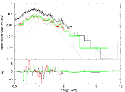
Figure 23: Two-temperature mekal fit to combined XMM-Newton PN and MOS1+2 spectra of DH Cep. An interstellar column of $N_{\rm H}=0.667\times 10^{22}\,{\rm cm^{-2}}$ has been assumed.

5.1.3 HD 215835 (DH Cep)

HD 215835 (DH Cep), located in the young open cluster NGC 7380, is an extremely tight O6V + O7V binary with a circular orbit of just 2.1109 d period (Penny, Gies & Bagnuolo 1997). The stars are tidally distorted, but at present are fully detached. The inclination remains slightly uncertain ($35^{\circ}<i<51^{\circ}$). The significant optical polarization is consistent with scattering within a WCR, while its short-term variability may be related to instabilities in the WCR (Corcoran 1991). An analysis of the wind ram pressures reveals that there is unlikely to be any balance, and the primary wind should directly impact the secondary star. However, once again a detailed simulation of this system will be necessary to place this hypothesis on a firmer footing.

DH Cep was observed by XMM-Newton on $19^{\rm th}$ December, 2003, for $\approx 30$ ksec with the MOS1 and MOS2 cameras, and $\approx 28$ ksec with the PN camera. It was reduced using standard scripts and version 9.0.0 of SAS, and the spectrum was rebinned to obtain a minimum of 25 counts per bin. Fig. 23 shows a two-temperature mekal fit, with an assumed ISM column of $0.667\times 10^{22}\,{\rm cm^{-2}}$, the weighted average returned by the NH tool at the HEASARC website. The fit is good ($\chi^{2}_{\nu}=1.18$), and has the following parameters: $kT_{1}=0.24^{+0.02}_{-0.01}$ keV, $kT_{2}=0.76^{+0.09}_{-0.06}$ keV, $N_{\rm H_{1}}=0.67^{+0.04}_{-0.00}\times 10^{22}\,{\rm cm^{-2}}$, $N_{\rm H_{2}}=1.05^{+0.17}_{-0.14}\times 10^{22}\,{\rm cm^{-2}}$, ${\rm norm_{1}}=2.07^{+0.73}_{-0.24}\times 10^{-3}$, and ${\rm norm_{2}}=4.29^{+0.80}_{-0.74}\times 10^{-4}$. The returned temperatures are similar to those from model cwb1. The fit needed no extra circumstellar absorption to the soft component (as also found for model cwb1), but favoured a circumstellar column of about $0.4\times 10^{22}\,{\rm cm^{-2}}$ to the hard component (again in good agreement with model cwb1). Assuming a distance of 3.73 kpc (Massey, Johnson & Degioia-Eastwood 1995), the ISM corrected $0.5-10$ keV luminosity is $6.3\times 10^{33}\,\hbox{${\rm{\rm\thinspace erg}{\rm\thinspace s}^{-1}\,}$}$. With ${\rm log}\,L_{\rm bol}=5.85$ (Penny et al. 1997), we obtain $L_{\rm x}/L_{\rm bol}=2.3\times 10^{-6}$. The X-ray luminosity and $L_{\rm x}/L_{\rm bol}$ values are slightly higher than obtained from model cwb1. It is entirely plausible that such a high X-ray luminosity could be obtained even if the primary wind crushes that of its companion, because in such a scenario the secondary star would nonetheless intercept a large fraction of the primary’s wind due to its proximity.

The slightly hotter temperature of the 2nd mekal component compared to model cwb1 may indicate that the primary wind indeed collides directly with the surface of the companion star, since it then has more room to accelerate before its collision, and thus the ability (ignoring potential braking and inhibition effects - see Gayley, Owocki & Cranmer (1997) and Stevens & Pollock (1994), respectively) to reach higher pre-shock speeds.

5.2 Intermediate and adiabatic systems

Systems with slightly longer orbital periods and wider stellar separations, some of which bear similarities to model cwb2, are now considered. Specifically, observations of HD 93161A and HD 47129 (Plaskett’s star) are discussed.

5.2.1 HD 93161A

HD 93161A is an O8V + O9V system with an orbital period of 8.566 d. The mimimum masses from the orbital solution are quite large, which suggests that the inclination of the orbit is high, most probably $>75^{\circ}$ (Nazé et al. 2005). The winds achieve a ram pressure balance, and both shocked winds are largely adiabatic (the primary’s more so: we estimate that $\chi_{1}\approx 30$ and $\chi_{2}\approx 5$).

The system was observed five times with XMM-Newton during 2000 and 2001, but no significant variations at energies above 0.5 keV were detected. This is nicely consistent with the theoretical lightcurves from model cwb2 shown in Fig. 3, which display little orbital variation in energy bands above 0.5 keV due to: i) the low attenuation through the circumstellar winds caused by the relatively low mass-loss rates and the relatively wide stellar separation, and ii) low occultation due to the large size of the WCR relative to the stars.

The observed luminosity in the $0.4-10$ keV band is $1.2\times 10^{32}\;\hbox{${\rm{\rm\thinspace erg}{\rm\thinspace s}^{-1}\,}$}$, which is an order of magnitude fainter than model cwb2. At first glance this would appear to be a big problem, but there are two important factors which can reconcile this issue. Firstly, the interstellar column to this system ($N_{\rm H}=4.5\times 10^{21}\;{\rm cm^{-2}}$) is significantly higher than assumed for our models. Secondly, the winds in this system are likely to be much more feeble compared to the O6V winds assumed in our model. Since the X-ray luminosity $L_{\rm x}\propto\hbox{${\dot{M}}$}^{2}$ in adiabatic systems, a reduction of a factor of 3 or so in the mass-loss rates would bring the observed and theoretical luminosities into better agreement. Such a reduction is consistent with the expected change in the mass-loss rate between an O6 and an O8/9 main-sequence star.

Nazé et al. (2005) find that two-temperature mekal fits to the X-ray spectra of HD 93161A yield average values of $kT_{1}=0.28\pm 0.02$ keV and $kT_{2}=0.76\pm 0.17$ keV. The derived circumstellar column varies between $0.45\times 10^{22}\;{\rm cm^{-2}}$ (at phases $0.18-0.53$) and $0.86\times 10^{22}\;{\rm cm^{-2}}$ (at phase 0.75). More recently, Antokhin et al. (2008) performed a 2-temperature fit to the combined data, finding temperatures of $0.27^{+0.02}_{-0.03}$ keV and $1.16^{+0.39}_{-0.24}$ keV. The hotter temperature from this fit is greater than the temperature of the hot component in any of the 5 individual spectra analyzed by Nazé et al. (2005). This highlights some of the non-uniqueness issues of spectral fits to medium-resolution spectra which is well documented in the literature.

In comparison, two-temperature mekal fits to model cwb2 are generally pretty poor (typically $\chi^{2}_{\nu}>2$), with three-temperatures needed to provide satisfactory fits. With this in mind, typical temperatures obtained from two-component fits are 0.25 keV and 1.4 keV, with the analysis of simulated Chandra spectra returning higher temperatures for the hotter component ($1.64$ keV and $1.68$ keV, at phase 0.0 and 0.25, respectively) than the corresponding analysis of a “fake” Suzaku dataset ($1.07$ keV and $1.35$ keV, at phase 0.0 and 0.25, respectively). Excluding one of the Suzaku analyzes, the values of $kT_{2}$ considerably exceed those reported from HD 93161A, even the higher value found by Antokhin et al. (2008). However, this is not too surprising given that the wind speeds of the O8V and O9V stars in HD 93161A are likely to be considerably lower than those assumed from the O6V stars in model cwb2.

5.2.2 HD 47129 (Plaskett’s star)

X-ray observations of systems containing evolved O-stars have also been presented in the recent literature. One notable analysis concerns Plaskett’s star (HD 47129), an O8III/I + O7.5III system with a circular orbit of period 14.4 d (Linder et al. 2008). The stars are very massive ($54\,\hbox{${\rm\thinspace M_{\odot}}$}$ and $56\,\hbox{${\rm\thinspace M_{\odot}}$}$ for the primary and secondary star respectively, assuming an orbital inclination of $71^{\circ}$). Linder et al. (2008) note that the secondary star is deformed due to its large rotational velocity, which results in a non-uniform temperature distribution, and speculate that the wind is confined near the equatorial plane. In this way the apex of the WCR can occur closer to the primary star (even if its wind has the overall greater mass-loss rate), as suggested from the analysis of optical emission lines (Wiggs & Gies 1992; Linder et al. 2008).

XMM-Newton observations of Plaskett’s star were presented by Linder et al. (2006). While there appears to be a minimum in the observed count rate when the primary star is in front, the amplitude of variability remains uncertain, as it is quite small between two XMM-Newton observations, but larger in archival ROSAT HRI observations. There is a pressing need for additional data to resolve this issue, and to examine whether there is an additional minimum during each orbit. The interstellar absorbing column is $1.5\times 10^{21}\;{\rm cm^{-2}}$ (Diplas & Savage 1994), similar to the value assumed for our models. The observed $0.5-10$ keV luminosity from the XMM-Newton observations ($6.9\times 10^{32}\;\hbox{${\rm{\rm\thinspace erg}{\rm\thinspace s}^{-1}\,}$}$) is also similar to the luminosities obtained in models cwb2 and cwb3, while a minimum in the luminosity near phase 0.0 is again consistent with the models.

There is some evidence (e.g. a very faint Fe K line) that the hot X-ray emitting plasma may not be in thermal equilibrium, or that there is a power-law tail to the hard emission. While the latter may indicate that non-thermal processes, such as particle acceleration, are occuring, it could also be an artifact of the fitting method: additional fits using a bremsstrahlung model to fit the continuum plus individual delta functions to fit the lines did not require a power-law component. The temperature returned for the bremsstrahlung component is $2.22\pm 0.1$ keV. Three-component mekal fits return temperatures of $0.31^{+0.02}_{-0.01}$ keV, $0.74^{+0.03}_{-0.02}$ keV and $2.42^{+0.39}_{-0.16}$ keV. No extra column was needed to the softest component, but circumstellar columns of $4.7^{+0.6}_{-0.7}\times 10^{21}\;{\rm cm^{-2}}$ and $3.0^{+1.3}_{-1.5}\times 10^{21}\;{\rm cm^{-2}}$ were needed for the intermediate and hard components, respectively.

The temperatures reported above are comparable to those obtained by three-temperature mekal fits to the synthetic spectra generated from models cwb2 and cwb3, and noted in Table 3. In addition, a lower column to the harder than to the intermediate component is consistent with the phase 0.25 results in Fig. 5(e). However, a specific model of this system is needed to determine whether all the observational data can be accurately reproduced.

5.3 Eccentric/unequal wind systems

We now discuss systems with eccentric orbits and/or unequal winds, bearing some similarities to models cwb3 and cwb4.

5.3.1 HD 93403

Four XMM-Newton observations of HD 93403, an O5.5I +O7V binary with a 15.093 d orbit of eccentricity $e=0.234$, reveal flux variations of 20 per cent amplitude in the $0.5-2.5$ keV band, with a minimum centered on apastron and a peak at periastron (Rauw et al. 2002a). In the softer $0.5-1.0$ keV band the minimum occurs at phase 0.75, when the denser wind of the O5.5I primary is in front. Variations in the harder $2.5-10$ keV band are less significant. Rauw et al. (2002a) found that HD 93403 appears less overluminous in X-rays than previously thought, and suggested that a significant fraction of the total X-ray emission may arise in line-instability shocks intrinsic to the winds. The orbital inclination is thought to be $\sim 30^{\circ}$.

The spectrum obtained nearest to periastron is not markedly softer than the spectra obtained at other phases. A two-temperature mekal fit yields temperatures of $\approx 0.23$ keV and 1.06 keV, with the harder component showing more variability. The observed luminosity (assuming a distance of 3.2 kpc) in the $0.5-10$ keV band is $\approx 1.6\times 10^{33}\,{\rm erg\;s^{-1}}$. The circumstellar column was found to be $\approx 8\times 10^{20}\,{\rm cm^{-2}}$ and $\approx 4.6\times 10^{21}\,{\rm cm^{-2}}$ to the soft and hard mekal components, respectively.

This system combines features of both models cwb3 and cwb4 (unequal winds and an eccentric orbit). However, unlike model cwb4, analysis of the wind ram pressures suggests that the winds may not be able to sustain a stable balance at periastron, with the result that the more powerful wind from the O5.5I star overwhelms that of its companion, and crashes directly onto its surface. Having said this, a full examination of the potential effects of radiative inhibition and braking is necessary to strengthen this hypothesis. Assuming that the primary wind does impact the companion star at periastron, it will be shocked to high temperatures, and should radiate reasonably efficiently ($\chi\sim 1$). A stable wind balance should be possible at apastron, but whether the O7V star can reestablish its wind towards its larger companion also remains to be seen. If a wind balance occurs, we estimate that both the shocked primary and secondary winds should be marginally adiabatic ($\chi_{1}\approx 2.5,\chi_{2}\approx 5$).

Bearing in mind that the nature of the WCR in this system could be quite different to that in models cwb3 and cwb4, we compare in the following the X-ray properties of this system with those from our models. We first note that the observed luminosity is approximately a factor of 2 greater than the luminosity from model cwb3, but is comparable to the luminosity from model cwb4 over most of the orbit, though the interstellar absorption column to HD 93403 at $3.67\times 10^{21}\,{\rm cm^{-2}}$ is higher than that assumed in our models. The circumstellar columns to the mekal components are comparable to the energy-dependent columns shown in Fig. 5(e). We can also make a direct comparison to the results of a two-temperature mekal fit to a simulated 10 ksec Suzaku observation of model cwb3 at $i=90^{\circ}$ and phase 0.0. Though such a fit is poor ($\chi^{2}_{\nu}=1.81$, with 224 d.o.f.), we find that the fit temperatures ($kT_{1}=0.26\pm 0.02$ keV, $kT_{2}=1.21\pm 0.05$ keV) are nevertheless roughly comparable to the values obtained from analysis of the observations of HD 93403. The circumstellar column to the cooler component is not in very good agreement ($N_{\rm H_{1}}=0.23^{+0.08}_{-0.07}\times 10^{22}\,{\rm cm^{-2}}$), though the column to the hotter component is a better match ($N_{\rm H_{2}}=0.31\pm 0.08\times 10^{22}\,{\rm cm^{-2}}$).

5.3.2 Cyg OB2#8A

Cyg OB2#8A is a longer period (21.9 d) O6If + 05.5III(f) binary with an orbital eccentricity $e=0.24$ (De Becker, Rauw & Manfroid 2004). It has long been known as a very bright X-ray source. XMM-Newton observations, together with archive ROSAT and ASCA data, reveal that the observed emission reaches a maximum near phase 0.75, with a minimum likely to occur shortly after periastron passage (De Becker et al. 2006). The intrinsic X-ray luminosity varies between $1.0-1.9\times 10^{34}\;\hbox{${\rm{\rm\thinspace erg}{\rm\thinspace s}^{-1}\,}$}$, giving an excess of $\sim 20$ compared to the canonical relationship for single stars. Clearly, this is caused by the collision of two very powerful winds. The orbital modulation of the emission matches roughly the $1/d_{\rm sep}$ variation expected if the winds are adiabatic. The emission is best fit by a 3-temperature mekal model with plasma temperatures of approximately $0.24\,$keV, $0.80\,$keV, and $1.76\,$keV, though the hottest component shows a significant decline in temperature (by about 15 per cent) between apastron and periastron.

While De Becker et al. (2006) estimated that the postshock winds would be radiative around the entire orbit, the assumed mass-loss rates may have been too high, and the terminal velocities too low. With mass-loss rates and terminal velocities more typical of recent determinations for the stellar types (e.g. Repolust, Puls & Herrero 2004; Martins et al. 2005a), we estimate that the primary wind possibly becomes radiative at periastron though is marginally adiabatic at apastron, while the secondary wind should remain adiabatic throughout the orbit.

Since the nature of the WCR in Cyg OB2#8A is clearly different to that in any of the models calculated in Paper I, it is unsurprising that the behaviour and characteristics of its X-ray emission do not closely match those from any of our models. Nevertheless, it is interesting to compare this system to our model cwb4 which also displays variations in its fit parameters (see Table 5 and Fig. 22). In model cwb4 the hot component from 3-temperature fits declines by 65 per cent, a much larger fall than seen from the actual observations of Cyg OB2#8A. That the variability is much lower in Cyg OB2#8A is likely due to smaller changes in the pre-shock wind speeds around the orbit (see Table 11 in De Becker et al. 2006) compared to model cwb4. In addition, the minimum temperature of the hot component in the fits to model cwb4 actually occurs after periastron (phase 0.05), this “time delay” being due to the history of the plasma temperature within the WCR. It would be interesting to obtain further X-ray observations of Cyg OB2#8A, with better phase coverage, to search for a similar effect, although the reduced eccentricity and longer orbital period may shorten or prevent a similar time delay from being seen. A specific hydrodynamical model of this system, which would allow further comparison of its emission in both the X-ray and radio domains (Cyg OB2#8A is also a strongly variable non-thermal radio source), would clearly be of interest.

5.3.3 HD 37043 ($\iota$ Ori)

$\iota$ Ori is a highly eccentric ($e=0.764$), O9III +B1III binary with a 29.134 d orbital period (Marchenko et al. 2000), which may have formed via an exchange of binary components in a binary-binary collision (Bagnuolo et al. 2001). It was observed twice by ASCA during 1997, with the observations timed to coincide with periastron and apastron (Pittard et al. 2000). The X-ray emission is bright because of its relative proximity ($D\sim 450$ pc). The observed $0.5-10$ keV luminosities are $\approx 1.0\times 10^{32}\,\hbox{${\rm{\rm\thinspace erg}{\rm\thinspace s}^{-1}\,}$}$ in both pointings. Since the wind attenuation is negligible, and the interstellar column is low ($N_{\rm H}=2\times 10^{20}\,{\rm cm^{-2}}$), the intrinsic X-ray luminosity of this system is also relatively low, consistent with the relatively feeble winds in this system. Surprisingly, there is no significant variation in the luminosity, spectral shape, or absorption between the periastron and apastron observations. Possible explanations for this lack of variability are that the WCR stays pinned to the surface of the secondary star throughout the entire orbit, or that intrinsic shocks within the winds generated by the radiatively driven line deshadowing instability dominate the emission (Pittard 1998).

5.4 Non-thermal X-ray emission

Since accelerated particles exist in many CWBs, the possibility of inverse Compton X-ray emission has previously been raised by a number of authors (e.g. Pollock 1987). Others have argued that non-thermal X-rays can be produced in the intrinsic wind shocks formed through the line-deshadowing instability (Chen & White 1991). A recent review of non-thermal emission processes in massive binaries can be found in De Becker (2007). However non-thermal X-rays might be produced, their detection requires that their flux become significant relative to the thermal X-ray flux. Unfortunately, a campaign focused on O-stars with known non-thermal radio emission failed to unambiguously detect any non-thermal X-ray’s at energies below 10 keV (Rauw et al. 2002b, 2005; De Becker et al. 2004c, 2005, 2006). Only from HD 159176 was possible evidence of a non-thermal component found (De Becker et al. 2004b). As noted in Sec. 5.1.2, this system has a very short period. The stellar winds likely collide at relatively low speeds, which limits the hardness of the thermal X-ray emission, allowing easier detection of a possible non-thermal component.

The chance of unambiguously detecting non-thermal X-ray’s increases with energy, as the emission from the thermal component falls off. It is partly for this reason that non-thermal X-ray emission has been reported from a Suzaku observation of $\eta$ Car (Sekiguchi et al. 2009). However, it appears that, at least in the soft ($E\mathrel{\hbox to0.0pt{\lower 3.0pt\hbox{$\sim$}\hss}\raise 2.0pt\hbox{$<$}}10\,$keV) domain, non-thermal X-rays are at best a relatively insignificant component

6 Summary and conclusions

This work investigates the X-ray emission from short-period O+O-star binaries where orbital effects and the acceleration of the winds are important. The structure and dynamics of the stellar winds and the wind-wind collision region for four distinct systems were previously calculated using a 3D hydrodynamical code (Paper I). We explore the emission arising from these models, under conditions where the WCR is radiative (model cwb1) or adiabatic (model cwb2), where the winds have unequal strengths (model cwb3), and where the orbit is eccentric (model cwb4).

We find that model cwb1 shows the greatest X-ray variability of the three models with circular orbits (models cwb1, cwb2 and cwb3), due to the closer stellar separation and the higher densities surrounding the WCR. The lightcurves from each of these models are asymmetrical because of orbit induced aberration and curvature of the WCR. The asymmetry is greatest for model cwb1, which has the highest ratio of orbital to wind speeds, $v_{\rm orb}/v_{\rm w}$, of the 3 simulations. The lightcurve asymmetry is always greatest for an observer located in the orbital plane ($i=90^{\circ}$), and generally decreases with decreasing $i$ (as does the level of variability). Model cwb4 shows that the X-ray emission from systems with eccentric orbits can be spectacularly variable, and can display a strong hysteresis around the orbit. In general, the emission is softer while the stars are separating after periastron passage, and harder when the stars are approaching. The degree of hysteresis, and its duration, likely depends on the amplitude of changes to the ratio of the orbital period to the flow time of the shocked plasma out of the system. As expected, the increase in the luminosity as periastron is approached does not follow the $1/d_{\rm sep}$ scaling of an adiabatic, terminal wind speeds, WCR. The observed change also depends on the energy band and the observer’s orientation. The ratio of the ISM corrected $0.5-10$ keV X-ray luminosity to the system bolometric luminosity, $L_{\rm x}/L_{\rm bol}$, reaches values as high as $5.9\times 10^{-6}$ under favourable viewing angles, consistent with a very strong colliding winds signature. All-in-all, the diversity and richness of the simulated X-ray lightcurves matches well their observational counterparts.

We use the difference between the intrinsic and attenuated spectra from the models to calculate “effective” circumstellar absorbing columns which we demonstrate can be extremely energy dependent. Therefore, simple spectral fits which assume energy independent columns are over-simplified in the same way that modelling the spectrum with only a handful of different plasma temperatures is, and risk compromising the subsequent interpretation. We also fold our theoretical spectra through the response files of the Chandra and Suzaku observatories, add poisson noise, and then analyze using the same method used for the analysis of real data. In many cases the fits return circumstellar columns in good agreement with the energy-dependent “effective” columns calculated directly from the theoretical spectra. However, there are also many instances where the returned columns have values which are not so close, and/or do not properly capture the trend of the effective circumstellar column with energy. We also find that despite our theoretical spectra being calculated with solar abundances, exclusively sub-solar values are returned by the spectral fitting package to our simulated spectra when the global abundance is allowed to fit freely. The global abundances become closer to the true (solar) value as the complexity of the spectral model increases. These issues highlight some of the problems associated with fitting overly simplified models to spectra, including non-uniqueness of the returned values, and of course are of wider significance than just CWBs. Moreover, the intrinsic luminosities inferred from very short period systems are often underestimated (by up to a factor of two), since the spectral models as used are unable to account for occultation losses. Despite these failings, in many cases the resulting fit parameters are, at least to first order, similar to those obtained from the analysis of real observations. More stringent comparisons between theory and observations will require the modelling of specific systems, such as work currently being conducted on $\eta$ Car.

In this paper we have examined the emission from main-sequence O+O-star systems, in which circumstellar absorption is relatively minor. Circumstellar absorption becomes more important as the stellar mass-loss rates increase, so that CWBs which contain a Wolf-Rayet (WR) star should display more significant orbital modulation of their lightcurves and spectra than seen in this work. For this reason, future work will explore the dynamics and emission from WR+O systems, where dynamical effects like radiative braking (Gayley et al. 1997) will also be important. It will also be interesting to explore other parts of the CWB parameter space. This could include: i) systems where a weaker wind is completely overwhelmed by a stronger wind (relevant to HD 93205, amongst others), ii) systems with an eccentric orbit where all (or one side) of the shocked plasma in the WCR is radiative throughout the entire orbit (relevant to systems like HD 155248, an O7.5(f)III + O7(f)III binary with a 5.816 d orbit of eccentricity 0.127 (Mayer et al. 2001), which shows strong phase-locked X-ray emission with an asymmetric modulation (Sana et al. 2004)), iii) systems with more than two stars (relevant to HD 167971 and QZ Car, amongst others).

This work has also been limited to simulating medium resolution X-ray spectra. Future work will examine X-ray line profiles, which can directly probe the dynamics deep in the WCR (Henley, Stevens & Pittard 2003, 2005, 2008), and interesting physics such as non-equilibrium ionization (e.g. Pollock et al. 2005) and non-equilibrium electron and ion temperatures (Zhekov & Skinner 2000). Further papers will examine the high energy non-thermal emission at X-ray and $\gamma$-ray energies up to the TeV range.

Despite this long to-do list, the present work has provided further essential groundwork, highlighting the factors which affect various aspects of the X-ray emission from short period O+O star binaries. It lays the foundations for a better understanding of some of the key physics of such systems (e.g. radiatively driven winds, high Mach number shocks), which will be studied with future models of particular systems.

References

- Anders & Grevesse (1989) Anders E., Grevesee N., 1989, GeCoA, 53, 197
- Antokhin et al. (2004) Antokhin I. I., Owocki S. P., Brown J. C., 2004, ApJ, 611, 434
- Antokhin et al. (2008) Antokhin I. I., Rauw G., Vreux J.-M., van der Hucht K. A., Brown J. C., 2008, A&A, 477, 593
- Arias et al. (2002) Arias J. I., Morrell N. I., Barbá R. H., Bosch G. L., Grosso M., Corcoran M., 2002, A&A, 333, 202
- Bagnuolo et al. (2001) Bagnuolo W. G. Jr., Riddle R. L., Gies D. R., Barry D. J., 2001, ApJ, 554, 362
- Blomme et al. (2007) Blomme R., De Becker M., Runacres M. C., Van Loo S., Setia Gunawan D. Y. A., 2007, A&A, 464, 701
- Blomme et al. (2005) Blomme R., Van Loo S., De Becker M., Rauw G., Runacres M. C., Setia Gunawan D. Y. A., Chapman J. M., 2005, A&A, 436, 1033
- Bouret et al. (2005) Bouret J.-C., Lanz T., Hillier D. J., 2005, A&A, 438, 301
- Castor, Abbott & Klein (1975) Castor J. I, Abbott D. C., & Klein R. I., 1975, ApJ, 195, 157 (CAK)
- Chen & White (1991) Chen W., White R. L., 1991, ApJ, 366, 512
- Corcoran (1991) Corcoran M. F., 1991, ApJ, 366, 308
- Corcoran (1996) Corcoran M. F., 1996, RevMexAA, 5, 54
- Damiani (2004) Damiani F., Flaccomio E., Micela G., Sciortino S., Harnden F. R. Jr., Murray S. S., 2004, ApJ, 608, 781
- De Becker (2007) De Becker M., 2007, A&ARv, 14, 171
- De Becker et al. (2005) De Becker M., Rauw G., Blomme R., Pittard J. M., Stevens I. R., Runacres M. C., 2005, A&A, 437, 1029
- De Becker, Rauw & Manfroid (2004) De Becker M., Rauw G., Manfroid J., 2004, A&A, 424, L39
- De Becker et al. (2004b) De Becker M., Rauw G., Pittard J. M., Antokhin I. I., Stevens I. R., Gosset E., Owocki S. P., 2004b, A&A, 416, 221
- De Becker et al. (2004c) De Becker M., et al., 2004c, A&A. 420, 1061
- De Becker et al. (2006) De Becker M., et al., 2006, MNRAS, 371, 1280
- Diplas & Savage (1994) Diplas A., Savage B. D., 1994, ApJS, 93, 211
- Dougherty et al. (2005) Dougherty S. M., Beasley A. J., Claussen M. J., Zauderer B. A., Bolingbroke N. J., 2005, ApJ, 623, 477
- Dougherty et al. (2003) Dougherty S. M., Pittard J. M., Kasian L., Coker R. F., Williams P. M., Lloyd H. M., 2003, A&A, 409, 217
- Dougherty, Williams & Pollacco (2000b) Dougherty S. M., Williams P. M., Pollacco D. L., 2000, MNRAS, 316, 143
- Ferland (2000) Ferland G., 2000, Rev. Mex. AA, 9, 153
- Fullerton et al. (2006) Fullerton A. W., Massa D. L., Prinja R. K., 2006, ApJ, 637, 1025
- Gayley et al. (1997) Gayley K. G., Owocki S. P., Cranmer S. R., 1997, ApJ, 475, 786
- Hamaguchi et al. (2007) Hamaguchi K., et al., 2007, ApJ, 663, 522
- Henley et al. (2008) Henley D. B., Corcoran M. F., Pittard J. M., Stevens I. R., Hamaguchi K., Gull T. R., 2008, ApJ, 680, 705
- Henley et al. (2003) Henley D. B., Stevens I. R., Pittard J. M., 2003, MNRAS, 346, 773
- Henley et al. (2005) Henley D. B., Stevens I. R., Pittard J. M., 2005, MNRAS, 356, 1308
- Lemaster et al. (2007) Lemaster M. N., Stone J. M., Gardiner T. A., 2007, ApJ, 662, 582
- Leyder et al. (2008) Leyder J.-C., Walter R., Rauw G., 2008, A&A, 477, L29
- Linder et al. (2006) Linder N., Rauw G., Pollock A. M. T., Stevens I. R., 2006, MNRAS, 370, 1623
- Linder et al. (2007) Linder N., Rauw G., Sana H., De Becker M., Gosset E., 2007, A&A, 474, 193
- Linder et al. (2008) Linder N., Rauw G., Martins F., Sana H., De Becker M., Gosset E., 2008, A&A, 489, 713
- Linder et al. (2009) Linder N., Rauw G., Manfroid J., Damerdji Y., De Becker M., Eenens P., Royer P., Vreux J.-M., 2009, A&A, submitted
- Luo et al. (1990) Luo D., McCray R., Mac Low M.-M., 1990, ApJ, 362, 267
- Marchenko et al. (2000) Marchenko S. V., et al., 2000, MNRAS, 317, 333
- Martins et al. (2005a) Martins F., Schaerer D., Hillier D. J., 2005a, A&A, 436, 1049
- Martins et al. (2005b) Martins F., Schaerer D., Hillier D. J., Meynadier F., Heydari-Malayeri M., Walborn N. R., 2005b, A&A, 441, 735
- Massey et al. (1995) Massey P., Johnson K. E., Degioia-Eastwood K., 1995, ApJ, 454, 151
- Mayer et al. (2001) Mayer P., Harmanec P., Lorenz R., Drechsel H., Eenens P., Corral L. J., Morrell N., 2001, in Vanbeveren D., ed., Astrophysics and Space Science Library (ASSL) 264, The Influence of Binaries on Stellar Population Studies. Kluwer, Dordrecht, p. 567
- Mayer et al. (2001b) Mayer P., Lorenz R., Drechsel H., Abseim A., 2001, A&A, 366, 558
- Mewe et al. (1995) Mewe R., Kaastra J. S., Liedahl D. A., 1995, Legacy, 6, 16
- Morrell et al. (2001) Morrell N. I., et al., 2001, MNRAS, 326, 85
- Myasnikov & Zhekov (1993) Myasnikov A. V., Zhekov S. A., 1993, MNRAS, 260, 221
- Nazé et al. (2005) Nazé Y., Antokhin I. I., Sana H., Gosset E., Rauw G., 2005, MNRAS, 359, 688
- Nazé et al. (2007) Nazé Y., Corcoran M. F., Koenigsberger G., Moffat A. F. J., 2007, ApJ, 658, L25
- Pachoulakis (1996) Pachoulakis I., 1996, MNRAS, 280, 153
- Parkin & Pittard (2008) Parkin E. R., Pittard J. M., 2008, MNRAS, 388, 1047
- Parkin et al. (2009) Parkin E. R., Pittard J. M., Corcoran M. F., Hamaguchi K., Stevens I. R., 2009, MNRAS, 394, 1758
- Pauldrach et al. (1986) Pauldrach A., Puls J., Kudritzki R. P., 1986, A&A, 154, 86
- Penny et al. (1997) Penny L. R., Gies D. R., Bagnuolo W. G. Jr., 1997, ApJ, 483, 439
- Pittard (1998) Pittard J. M., 1998, MNRAS, 300, 479
- Pittard (2007) Pittard J. M., 2007, ApJ, 660, L141
- Pittard (2009a) Pittard J. M., 2009a, MNRAS, 396, 1743 (Paper I)
- Pittard (2009b) Pittard J. M., 2009b, MNRAS, accepted (Paper II)
- Pittard (2009c) Pittard J. M., 2009c, in J. Martí, P. L. Luque-Escamilla, J. A. Combi, eds., ASPCS, High Energy Phenomena in Massive Stars
- Pittard & Corcoran (2002) Pittard J. M., Corcoran M. F., 2002, A&A, 383, 636
- Pittard & Dougherty (2006) Pittard J. M., Dougherty S. M., 2006, MNRAS, 372, 801
- Pittard et al. (2006) Pittard J. M., Dougherty S. M., Coker R. F., O’Connor E., Bolingbroke N. J., 2006, A&A, 446, 1001
- Pittard & Stevens (1997) Pittard J. M., Stevens I. R., 1997, MNRAS, 292, 298
- Pittard & Stevens (2002) Pittard J. M., Stevens I. R., 2002, A&A, 388, L20
- Pittard et al. (2000) Pittard J. M., Stevens I. R., Corcoran M. F., Gayley K. G., Marchenko S. V., Rauw G., 2000, MNRAS, 319, 137
- Pittard et al. (1998) Pittard J. M., Stevens I. R., Corcoran M. F., Ishibashi K., 1998, MNRAS, 299, L5
- Pittard et al. (2002c) Pittard J. M., Stevens I. R., Williams P. M., Pollock A. M. T., Skinner S. L., Corcoran M. F., Moffat A. F. J., 2002c, A&A, 388, 335
- Pollock (1987) Pollock A. M. T., 1987, A&A, 171, 135
- Pollock et al. (2005) Pollock A. M. T., Corcoran M. F., Stevens I. R., Williams P. M., 2005, ApJ, 629, 482
- Pollock & Corcoran (2006) Pollock A. M. T., Corcoran M. F.,2006, A&A, 445, 1093
- Puls et al. (2008) Puls J., Vink J. S., Najarro F., 2008, A&ARv, 16, 209
- Rauw et al. (2002a) Rauw G., Vreux J.-M., Stevens I. R., Gosset E., Sana H., Jamar C., Mason K. O., 2002a, A&A, 388, 552
- Rauw et al. (2002b) Rauw G., et al., 2002b, A&A, 394, 993
- Rauw et al. (2002c) Rauw G., Nazé Y., Gosset E., Stevens I. R., Blomme R., Corcoran M. F., Pittard J. M., Runacres M. C., 2002c, A&A, 388, 552
- Rauw et al. (2005) Rauw G., De Becker M., Linder N., 2005, in G. Rauw, Y. Nazé, R. Blomme, E. Gosset, eds., Proceedings of JENAM 2005, Massive Stars and High-Energy Emission in OB Associations, p. 103
- Repolust, Puls & Herrero (2004) Repolust T., Puls J., Herrero A., 2004, A&A, 415, 349
- Sana et al. (2004) Sana H., Stevens I. R., Gosset E., Rauw G., Vreux J.-M., 2004, MNRAS, 350, 809
- Sana et al. (2008) Sana H., Naze Y., O’Donnell B., Rauw G., Gosset E., 2008, New Ast., 13, 202
- Schild et al. (2004) Schild H., et al., 2004, A&A, 422, 177
- Sekiguchi et al. (2009) Sekiguchi A., Tsujimoto M., Kitamoto S., Ishida M., Hamaguchi K., Mori H., Tsuboi Y., 2009, PASJ, 61, 629
- Stevens et al. (1992) Stevens I. R., Blondin J. M., Pollock A. M. T., 1992, ApJ, 386, 265
- Stevens et al. (1996) Stevens I. R., Corcoran M. F., Willis A. J., Skinner S. L., Pollock A. M. T., Nagase F., Koyama K., 1996, MNRAS, 283, 589
- Stevens & Pollock (1994) Stevens I. R., Pollock A. M. T., 1994, MNRAS, 269, 226
- Strickland & Stevens (1998) Strickland D. K., Stevens I. R., 1998, MNRAS, 297, 747
- Van Loo et al. (2008) Van Loo S., Blomme R., Dougherty S. M., Runacres M. C., 2008, A&A, 483, 585
- Walder (1998) Walder R., 1998, Ap&SS, 260, 243
- White & Becker (1995) White R. L., Becker R. H., 1995, ApJ, 451, 352
- Wiggs & Gies (1992) Wiggs M. S., Gies D. R., 1992, ApJ, 396, 238
- Williams et al. (1997) Williams P. M., Dougherty S. M., Davis R. J., van der Hucht K. A., Bode M. F., Setia Gunawan D. Y. A., 1997, MNRAS, 289, 10
- Williams et al. (1992) Williams P. M., van der Hucht K. A., Bouchet P., Spoelstra T. A. Th., Eenens P. R. J., Geballe T. R., Kidger M. R., Churchwell E., 1992, MNRAS, 258, 461
- Zhekov & Skinner (2000) Zhekov S. A., Skinner S. L., 2000, ApJ, 538, 808