INSTABILITIES INDUCED BY PHASE FRONTS COALESCENCE DURING THE PHASE TRANSITIONS IN A THIN SMA LAYER: MECHANISM AND ANALYTICAL DESCRIPTIONS

Abstract

Systematic experiments on stress-induced phase transitions in thin SMA structures in literature have revealed two interesting instability phenomena: the coalescence of two martensite-austenite fronts leads to a sudden stress drop and that of two austenite-martensite fronts leads to a sudden stress jump. In order to get an insight into these two phenomena, in this work we carry out an analytical study on the stress-induced phase transitions in a thin SMA layer (a simple structure in which the two coalescence processes can happen). We derive a quasi-2D model with a non-convex effective strain energy function while taking into account the rate-independent dissipation effect. By using a coupled series-asymptotic expansion method, we manage to express the total energy dissipation in terms of the leading-order term of the axial strain. The equilibrium equations are obtained by maximizing the total energy dissipation, which are then solved analytically under suitable boundary conditions. The analytical results reveal that the mechanism for such instabilities is the presence of ”limited points”, which cause the switch of nontrivial solution modes to trivial solution modes. Descriptions for the whole coalescence processes of two fronts are also provided based on the analytical solutions, which also capture the morphology varies of the specimen. It is also revealed the key role played by the thickness-length ratio on these instabilities: the zero limit of which can lead to the smooth switch of nontrivial modes to trivial modes with no stress drop or stress jump.

1 Introduction

Systematic experiments on stress-induced phase transitions in thin SMA structures, such as wires, strips and tubes, have been carried out (Lexcellent $\&$ Tobushi 1995; Shaw $\&$ Kyriakides 1995, 1997; Sun et al 2000; Favier et al 2001; Li $\&$ Sun 2002; Feng $\&$ Sun 2006). In general, the whole experimental process can be divided into three stages. In the first stage, the deformation of the specimen is the elastic deformation of initial phase. In the second stage, the product phase first nucleates at some special site, and then propagates gradually along the specimen. Finally, the phase fronts coalescence and the whole length of the specimen has transformed to the product phase. In the third stage, the deformation of the specimen is the elastic deformation of the product phase. It was also found that the measured engineering stress-strain curves have some key features, e.g., the nucleation stress peak (for the loading case) and stress valley (for the unloading case), the stress plateaus, the rate-independent hysteresis loop and so on.

In this paper, we shall focus on the instability phenomena induced by the coalescence of two phase fronts. During the experiments, these instability phenomena can be easily identified from both the stress-strain curves and the surface morphology of the specimens (Shaw $\&$ Kyriakides 1997; Feng $\&$ Sun 2006). Systematic experimental results have obviously shown that the coalescence process is inevitably accompanied the varies of the stress value and the surface morphology of the specimen. In general, the coalescence process has the following procedure as described in Feng $\&$ Sun (2006). In the loading (unloading) case, as the total elongation increases (decreases), two martensite-austenite (austenite-martensite) phase fronts move towards each other. The austenite (martensite) region sandwiched between the phase fronts becomes more and more narrow. Eventually these two fronts start getting touch each other and the coalescence process takes place. It is clear the coalescence process is a dynamic process and seemingly uncontrollable in the sense that it occurs very rapidly (this may indicate that an instability occurs). During the coalescence process, the local configuration of the specimen transforms from an inhomogeneous mode to a homogeneous mode and the corresponding stress value has a rapid drop for the loading case and a rapid jump for the unloading case.

In order to get an insight into the phase fronts coalescence phenomena, in this work we carry out an analytical study on the stress-induced phase transitions in a thin SMA layer (a simple structure in which the two coalescence processes can happen). We shall derive a quasi-2D continuum model with a non-convex effective strain energy function while taking into account the rate-independent dissipation effect. The starting point of our model is the formulation of Rajagopal $\&$ Srinivasa (1999, 2004) (also see the formulation of Sun $\&$ Hwang 1993a, b). In fact, we have already proposed a quasi-3D continuum model earlier to study the phase transitions induced by extension in a slender SMA cylinder (see Wang $\&$ Dai 2009), which has almost the same formulation with this current model. Thus, we shall only give a brief introduction to the derivation procedure in this paper and the detailed derivation procedure can be found in Wang $\&$ Dai (2009).

In the experiments, typically the thickness-length (or width-length or radius-length) ratio of the specimen is of order $O(10^{-2})$. As a result, one might think that the deformation along the lateral direction can be neglected and the layer can be treated as a one-dimensional object. However, sometimes a purely one-dimensional model appears to be not sophisticated enough to capture some key features observed in experiments. Some explanations have already been given in Dai $\&$ Cai (2006). In this paper, the total elastic potential energy of the layer will be considered based on a two-dimensional setting. Starting from the two-dimensional governing system and by using the coupled series-asymptotic expansion method (Dai $\&$ Cai 2006; Cai $\&$ Dai 2006), we manage to express the total elastic potential energy of the layer in terms of the leading order term of the axial strain (cf. (3.41)). Although the final expression of the total elastic potential energy is one-dimensional, it takes into account the lateral deformation and has the higher-dimensional effects built in.

To describe the hysteretic behavior during the phase transition process, one also needs to consider the inevitable mechanical dissipation effect. In this paper, the mechanical dissipation effect will be considered in a purely one-dimensional setting, i.e., we neglect the influence of the radial deformation on the mechanical dissipation. A specific constitutive form of the rate of dissipation function is adopted in our model (cf. (2.6)). Based on the phase transition criteria and the criterion of maximum rate of dissipation, we propose the evolution laws of the phase state variable for the purely loading and purely unloading processes. After doing some further analysis, we derive the one-dimensional expressions for the mechanical dissipation functions in terms of the axial strain (cf. (4.5)-(4.8)).

With the expressions of the total elastic potential energy and the mechanical dissipation functions, the equilibrium configurations of the layer for the purely loading and purely unloading processes can be determined by using the principle of maximizing the total energy dissipation. By using the variational method, we derive the equilibrium equations, which are then solved analytically under suitable boundary conditions. It will be seen that the solutions obtained show qualitatively agreements with the experimental results.

Based on the analytical solutions obtained and by using the limit-point instability criterion, we further consider the phase fronts coalescence process. It is revealed that during the coalescence process, the configurations of the layer switched from the nontrivial solution modes to the trivial solution modes, which is caused by the presence of the “limit points”. The morphology varies of the layer and the accompanying stress drop/jump during the coalescence process can be described. The influence of the thickness-length ratio of the specimen on the coalescence process is also studied. It will be shown that the zero limit of the thickness-length ratio can lead to the smooth switch of nontrivial solutions to trivial solutions with no stress drop or stress jump.

This paper is arranged as follows. In section 2, we give a simple introduction to the formulation of Rajagopal $\&$ Srinivasa (1999, 2004) and propose the evolution laws of the phase state variable for the purely loading and purely unloading processes. In section 3, we formulate the field equations by treating the thin layer as a two-dimensional object. By using the coupled series-asymptotic expansion method, we express the total elastic potential energy of the layer in terms of the asymptotic axial strain. In section 4, we study the mechanical dissipation effect. After some analysis, we express the mechanical dissipation functions in terms of the axial strain. In section 5, we derive the equilibrium equation by using the principle of maximizing the total energy dissipation. Then, we construct the analytical solutions for an illustrative example. In section 6, we further study the instability phenomena induced by phase fronts coalescence. We try to give some descriptions and explanations for the origin of the instability during the coalescence process, the accompanying stress drop/jump and the morphology varies of the specimen. We also consider the size-effect of the specimens on the coalescence process. Finally, some conclusions are drawn.

2 Preliminaries

In this section, we shall give a simple introduction to the formulation of Rajagopal $\&$ Srinivasa (1999, 2004), which is the starting point of our present model.

First, based on the balance laws and the local form of the entropy production equation, one can obtain the reduced energy-rate of dissipation relation as

$$-(\dot{\hat{\Psi}}+\dot{T}\eta)+\textrm{tr}(\mathbf{\Sigma}\dot{\mathbf{F}})=\zeta.\ \ \$$

In equation (2.1), $\hat{\Psi}$ is the Helmholtz free energy per unit referential volume, $T$ is the absolute temperature, $\eta$ is the entropy per unit volume in the reference configuration and $\zeta$ is the rate of mechanical dissipation, $\mathbf{F}$ is the deformation gradient tensor and $\mathbf{\Sigma}$ is the nominal stress tensor. The superposed dot indicates the material time derivative.

To describe the phase transition process, one also needs to adopt the phase state variable $\alpha$, which represents the volume fraction of the martensite phase in the reference configuration. It is assumed that $\hat{\Psi}$, $\mathbf{\Sigma}$ and $\eta$ depend on the variables $\{\mathbf{F},\alpha,T\}$, while the rate of mechanical dissipation $\zeta$ depends on $\{T,\alpha,\dot{\alpha}\}$. With these constitutive assumptions, the reduced energy-rate of dissipation relation (2.1) can be rewritten as

$$\textrm{tr}((\mathbf{\Sigma}-\frac{\partial\hat{\Psi}}{\partial\mathbf{F}})\dot{\mathbf{F}})-(\frac{\partial\hat{\Psi}}{\partial T}+\eta)\dot{T}-\frac{\partial\hat{\Psi}}{\partial\alpha}\dot{\alpha}=\zeta,$$

Equation (2.2) must hold for all $\dot{\mathbf{F}}$ and $\dot{T}$, thus one can arrive at the following constitutive equations:

$$\mathbf{\Sigma}=\frac{\partial\hat{\Psi}(\mathbf{F},\alpha,T)}{\partial\mathbf{F}},\ \$$

$$\eta=-\frac{\partial\hat{\Psi}(\mathbf{F},\alpha,T)}{\partial T},\ \$$

and

$$-\frac{\partial\hat{\Psi}(\mathbf{F},\alpha,T)}{\partial\alpha}\dot{\alpha}=\zeta.\ \$$

Once the specific forms of the functions $\hat{\Psi}$ and $\zeta$ are given, the nominal stress tensor $\mathbf{\Sigma}$ and entropy $\eta$ can be calculated from (2.3) and (2.4). Equation (2.5) provides the equation for the evolution of phase state variable $\alpha$. As we just consider the isothermal responses of SMA materials in this paper, the temperature $T$ will be considered as a given constant in the sequel.

In the paper of Rajagopal $\&$ Srinivasa (1999), the following constitutive form of the mechanical dissipation rate $\zeta$ was proposed

$$\zeta=\left\{\begin{aligned} &A^{+}(\alpha)|\dot{\alpha}|,\ \ \ \ \ \ &\textrm{if}\ \ \dot{\alpha}>0,\\ &0,\ \ \ \ \ \ \ \ \ \ \ \ \ \ \ \ &\textrm{if}\ \ \dot{\alpha}=0,\\ &A^{-}(\alpha)|\dot{\alpha}|,\ \ \ \ \ \ &\textrm{if}\ \ \dot{\alpha}<0,\end{aligned}\right.$$

where $A^{+}(\alpha)\geq 0$ and $A^{-}(\alpha)\geq 0$ referred to as the forward and backward dissipative resistances, respectively. An important consequence of (2.6) is that the response of the material is rate-independent, i.e., the stress-strain curve is the same irrespective of the speed with which the test is conducted.

Substituting (2.6) into (2.5) and using the fact that the resulting equation must be valid for all admissible processes, one can arrive at the following phase transition criteria

$$-A^{-}(\alpha)<-\frac{\partial\hat{\Psi}}{\partial\alpha}<A^{+}(\alpha)\Rightarrow\dot{\alpha}=0,\ \$$

$$\dot{\alpha}\neq 0\Rightarrow-\frac{\partial\hat{\Psi}}{\partial\alpha}=\left\{\begin{aligned} &A^{+}(\alpha),\ \ \ &\textrm{if}\ \ \dot{\alpha}>0,\\ &-A^{-}(\alpha),\ \ \ &\textrm{if}\ \ \dot{\alpha}<0.\end{aligned}\right.$$

Condition (2.7) represents the fact that as long as $-\partial\hat{\Psi}/\partial\alpha$ lies between $-A^{-}$ and $A^{+}$, no phase transition can take place. On the other hand, whenever $\dot{\alpha}\neq 0$, $-\partial\hat{\Psi}/\partial\alpha$ must equal to one of the dissipative resistances. At the two critical points $-\partial\hat{\Psi}/\partial\alpha=A^{+}$ or $-\partial\hat{\Psi}/\partial\alpha=-A^{-}$, the response of material may not be unique (Rajagopal $\&$ Srinivasa 1999, 2004). To fully determine the commencement and cessation of the phase transitions, one need to use the criterion of maximum rate of dissipation (Rajagopal $\&$ Srinivasa 1998, 1999). Intuitively speaking, the maximum rate of dissipation criterion states that if the material is capable of responding in many different modes with different rates of dissipations (including a mode that is non-dissipative), then the actual mode will be the one with the maximum rate of dissipation.

In general, there does not exist a one-to-one mapping between $\mathbf{F}$ and $\alpha$. Based on the phase transition criteria and the criterion of maximum rate of dissipation, we find that for a given deformation gradient $\mathbf{F}$, there may exist two phase state values $\alpha^{+}_{\mathbf{F}}$ and $\alpha^{-}_{\mathbf{F}}$ such that $-\partial\hat{\Psi}(\mathbf{F},\alpha^{+}_{\mathbf{F}})/\partial\alpha=A^{+}(\alpha^{+}_{\mathbf{F}})$ and $-\partial\hat{\Psi}(\mathbf{F},\alpha^{-}_{\mathbf{F}})/\partial\alpha=-A^{-}(\alpha^{-}_{\mathbf{F}})$, then the actual phase state $\alpha$ should satisfy $\alpha^{+}_{\mathbf{F}}\leq\alpha\leq\alpha^{-}_{\mathbf{F}}$.

In this paper, we shall only consider two kinds of loading patterns: the purely loading process with the initial state of the cylinder composed of austenite phase and the purely unloading process with the initial state of the cylinder composed of martensite phase. In the figure of the stress-strain response, the curves corresponding to these two kinds of loading patterns form the entire ‘outer loop’.

From the experiments, it was found that the deformation process at any material point can be divided into the elastic deformation process of the austenite phase, the elastic deformation process of the martensite phase and the phase transition process. The experimental results also reveal that the profile of the phase transition (localization) region has a stable form during the phase transition process. Thus, it is reasonable to impose the following assumption:

Assumption 1. In a quasi-static purely loading or purely unloading process, for the material points located in the phase transition region, it is satisfied that $\dot{\alpha}>0$ (for the loading process) or $\dot{\alpha}<0$ (for the unloading process).

With this assumption, we can propose the following relationship between $\alpha$ and $\mathbf{F}$ for the purely loading and unloading processes, respectively:

$$\alpha^{+}(\mathbf{F})=\left\{\begin{aligned} &0,\ \ \ \ \ \ \ \ \ \ \ \ \ \textrm{if}\ \ \ -\frac{\partial\hat{\Psi}(\mathbf{F},\alpha)}{\partial\alpha}|_{\alpha=0}\leq A^{+}(0),\\ &1,\ \ \ \ \ \ \ \ \ \ \ \ \ \textrm{if}\ \ \ -\frac{\partial\hat{\Psi}(\mathbf{F},\alpha)}{\partial\alpha}|_{\alpha=1}\geq A^{+}(1),\\ &\alpha^{+}_{\mathbf{F}},\ \ \ \ \ \ \ \ \ \ \ \textrm{if}\ \ \exists\ \alpha^{+}_{\mathbf{F}}\in(0,1),\ \ \textrm{s.t.},\ \ -\frac{\partial\hat{\Psi}(\mathbf{F},\alpha)}{\partial\alpha}|_{\alpha=\alpha^{+}_{\mathbf{F}}}=A^{+}(\alpha^{+}_{\mathbf{F}}).\end{aligned}\right.$$

$$\alpha^{-}(\mathbf{F})=\left\{\begin{aligned} &0,\ \ \ \ \ \ \ \ \ \ \ \ \ \textrm{if}\ \ \ -\frac{\partial\hat{\Psi}(\mathbf{F},\alpha)}{\partial\alpha}|_{\alpha=0}\leq-A^{-}(0),\\ &1,\ \ \ \ \ \ \ \ \ \ \ \ \ \textrm{if}\ \ \ -\frac{\partial\hat{\Psi}(\mathbf{F},\alpha)}{\partial\alpha}|_{\alpha=1}\geq-A^{-}(1),\\ &\alpha^{-}_{\mathbf{F}},\ \ \ \ \ \ \ \ \ \ \ \textrm{if}\ \ \exists\ \alpha^{-}_{\mathbf{F}}\in(0,1),\ \ \textrm{s.t.},\ \ -\frac{\partial\hat{\Psi}(\mathbf{F},\alpha)}{\partial\alpha}|_{\alpha=\alpha^{-}_{\mathbf{F}}}=-A^{-}(\alpha^{-}_{\mathbf{F}}).\end{aligned}\right.$$

3 The total elastic potential energy

In this section, we shall derive an “effective” one-dimensional expression for the total elastic potential energy of the layer, which takes into account the higher-dimensional effects.

We consider the symmetric deformation of a thin SMA layer subject to a static axial force at two ends. This layer can be considered as a cross-section cutting along the axial direction of a thin SMA strip or tube. Although here we just consider a very simple model as we treat this layer as a two-dimensional object, it will be seen that this simple model can capture some important experimental features.

Assume that in the stress-free configuration, the layer has thickness $2a$ and length $l$, where $a/l=\delta\ll 1$. We denote $(X,Y)$ and $(x,y)$ the coordinates of a material point of the layer in the reference and current configurations, respectively. The finite displacements can be written as

$$U(X,Y)=x(X,Y)-X,\ \ \ W(X,Y)=y(X,Y)-Y.\ \$$

As here we only consider the symmetric deformation of this layer, thus $U$ and $V$ have the following properties

$$U(X,-Y)=U(X,Y),\ \ \ W(X,-Y)=-W(X,Y).$$

Then the deformation gradient tensor $\mathbf{F}$ is given by

$$\mathbf{F}=(1+U_{X})\mathbf{e}_{1}\otimes\mathbf{E}_{1}+U_{Y}\mathbf{e}_{1}\otimes\mathbf{E}_{2}+W_{X}\mathbf{e}_{2}\otimes\mathbf{E}_{1}+(1+W_{Y})\mathbf{e}_{2}\otimes\mathbf{E}_{2},\ \$$

where $\{\mathbf{E}_{i}\}_{i=1,2}$ and $\{\mathbf{e}_{j}\}_{j=1,2}$ are the orthonormal base vectors in the reference and current configurations.

Based on (2.3), (2.9) and (2.10), we obtain that the nominal stress tensor $\mathbf{\Sigma}$ for the purely loading or purely unloading process should be given by

$$\mathbf{\Sigma}^{\pm}=\frac{\partial\hat{\Psi}(\textbf{F},\alpha)}{\partial\textbf{F}}|_{\alpha=\alpha^{\pm}(\textbf{F})}=:\textbf{G}^{\pm}(\textbf{F}),\ \$$

where $\mathbf{G}^{\pm}$ are tensor-valued functions. It will be assumed that there exist some “effective” strain energy functions $\Psi^{\pm}(\mathbf{F})$ such that

$$\mathbf{\Sigma}^{\pm}=\mathbf{G}^{\pm}(\mathbf{F})=\frac{\partial\Psi^{\pm}(\mathbf{F})}{\partial\mathbf{F}}.\ \ \$$

In this section, the purpose is to derive an “effective” one-dimensional expression for the elastic potential energy of the layer. Thus, we only consider the nondissipative case in this section, i.e., we assume $A^{\pm}(\alpha)=0$. From (2.9) and (2.10), it is easy to see that in the nondissipative case, the phase state functions satisfy $\alpha^{+}(\mathbf{F})=\alpha^{-}(\mathbf{F})=:\alpha(\mathbf{F})$. Further by using (2.9), (2.10) and (3.3), we have

$$\mathbf{\Sigma}(\mathbf{F}) =\frac{\partial\hat{\Psi}}{\partial\mathbf{F}}(\mathbf{F},\alpha)|_{\alpha=\alpha(\mathbf{F})}$$

$$=\frac{\partial\hat{\Psi}}{\partial\mathbf{F}}(\mathbf{F},\alpha(\mathbf{F}))-\frac{\partial\hat{\Psi}}{\partial\alpha}(\mathbf{F},\alpha)|_{\alpha=\alpha(\mathbf{F})}\cdot\frac{\partial\alpha(\mathbf{F})}{\partial\mathbf{F}}$$

$$=\frac{\partial\hat{\Psi}(\mathbf{F},\alpha(\mathbf{F}))}{\partial\mathbf{F}}.$$

The final equation in (3.5) is due to the fact that if $\mathbf{F}$ takes value in the phase transition domain, we have $-\frac{\partial\hat{\Psi}}{\partial\alpha}(\mathbf{F},\alpha)|_{\alpha=\alpha(\mathbf{F})}=0$, otherwise $\alpha(\mathbf{F})$ should be a constant function of $\mathbf{F}$.

From (3.5), we can see that the “effective” strain energy function in the nondissipative case should be given by

$$\Psi(\mathbf{F})=\hat{\Psi}(\mathbf{F},\alpha(\mathbf{F})).$$

In the sequel, we refer $\Psi(\mathbf{F})$ as the elastic potential energy function. To go further, we propose another important assumption:

Assumption 2. In the nondissipative case, SMA material can be considered as some kind of isotropic hyperelastic material. In this case, the elastic potential energy $\Psi(\mathbf{F})$ only depends on the two principle stretches $\lambda_{1}$, $\lambda_{2}$ of $\mathbf{F}$; that is $\Psi=\Psi(\lambda_{1},\lambda_{2})$.

If the components of $\mathbf{F}-\mathbf{I}$ are relatively small, it is possible to expand the nominal stress components in term of the strains up to any order. The formula containing terms up to the third order material nonlinearity is (cf. Fu $\&$ Ogden 1999)

$$\Sigma_{ji}=a_{jilk}^{1}\kappa_{kl}+\frac{1}{2}a^{2}_{jilknm}\kappa_{kl}\kappa_{mn}+\frac{1}{6}a^{3}_{jilknmqp}\kappa_{kl}\kappa_{mn}\kappa_{pq}+O(|\kappa_{st}|^{4}),\ \$$

where $\kappa_{ij}$ is the components of the tensor $\mathbf{F}-\mathbf{I}$ and

$$a_{jilk}^{1}=\frac{\partial^{2}{\Psi}}{\partial F_{ij}\partial F_{kl}}|_{\mathbf{F}=\mathbf{I}},\ \ \ \ a_{jilknm}^{2}=\frac{\partial^{3}{\Psi}}{\partial F_{ij}\partial F_{kl}\partial F_{mn}}|_{\mathbf{F}=\mathbf{I}},$$

$$a^{3}_{jilknmqp}=\frac{\partial^{4}{\Psi}}{\partial F_{ij}\partial F_{kl}\partial F_{mn}\partial F_{pq}}|_{\mathbf{F}=\mathbf{I}}$$

are incremental elastic moduli, which can be calculated once a specific form of elastic potential energy is given. From the formula (3.7), we can obtain the nominal stress components $\Sigma_{ji}$. For example,

$$\Sigma_{11}= \tau_{2}W_{Y}+\tau_{1}U_{X}$$

$$+\frac{1}{2}(\eta_{3}U_{Y}^{2}+\eta_{2}W_{Y}^{2}+2\eta_{2}W_{Y}U_{X}+\eta_{1}U_{X}^{2}+2\eta_{4}U_{Y}W_{X}+\eta_{3}W_{X}^{2})$$

$$+\frac{1}{6}(3\theta_{3}U_{Y}^{2}W_{Y}+\theta_{2}W_{Y}^{3}+3\theta_{3}U_{Y}^{2}U_{X}+3\theta_{5}W_{Y}^{2}U_{X}+3\theta_{2}W_{Y}U_{X}^{2}$$

$$+\theta_{1}U_{X}^{3}+6\theta_{7}U_{Y}W_{Y}U_{X}+6\theta_{4}U_{Y}U_{X}W_{X}+3\theta_{6}W_{Y}W_{X}^{2}+3\theta_{3}U_{X}W_{X}^{2}),$$

where $\tau_{i}$, $\eta_{j}$ and $\theta_{k}$ are some elastic moduli, whose formulas are given in appendix A. Owing to the complexity of calculations, we shall only work up to the third-order material nonlinearity. In the experiments, the maximum strain is less than $10\%$, and such an approximation is accurate enough, certainly not worse than the trilinear approximation adopted in many works.

For a static equilibrium configuration, the nominal stress tensor $\mathbf{\Sigma}$ satisfies the field equations

$$\textrm{Div}(\mathbf{\Sigma})=0,$$

which yields the following two equations

$$\frac{\partial\Sigma_{11}}{\partial X}+\frac{\partial\Sigma_{21}}{\partial Y}=0,\ \$$

$$\frac{\partial\Sigma_{12}}{\partial X}+\frac{\partial\Sigma_{22}}{\partial Y}=0.\ \$$

We consider the traction-free boundary conditions at $Y=\pm a$, i.e.,

$$\Sigma_{21}|_{Y=\pm a}=0,\ \ \ \ \Sigma_{22}|_{Y=\pm a}=0.\ \$$

Equations (3.9) and (3.10) together with (3.11) provide the governing equations for two unknowns $U$ and $W$.

We can also expand the elastic potential energy $\Psi$ in terms of the strains up to any order. The formula containing terms up to the fourth-order nonlinearity is given by

$$\Psi= \frac{1}{2}(\tau_{3}U_{Y}^{2}+\tau_{1}W_{Y}^{2}+2\tau_{2}W_{Y}U_{X}+\tau_{1}U_{X}^{2}+2\tau_{3}U_{Y}W_{X}+\tau_{3}W_{X}^{2})$$

$$+\frac{1}{6}(3\eta_{3}U_{Y}^{2}W_{Y}+\eta_{1}W_{Y}^{3}+3\eta_{3}U_{Y}^{2}U_{X}+3\eta_{2}W_{Y}^{2}U_{X}+3\eta_{2}W_{Y}U_{X}^{2}$$

$$+\eta_{1}U_{X}^{3}+6\eta_{4}U_{Y}W_{Y}W_{X}+6\eta_{4}U_{Y}U_{X}W_{X}+3\eta_{3}W_{Y}W_{X}^{2}+3\eta_{3}U_{X}W_{X}^{2})$$

$$+\frac{1}{24}(\theta_{8}U_{Y}^{4}+6\theta_{3}U_{Y}^{2}W_{Y}^{2}+\theta_{1}W_{Y}^{4}+12\theta_{6}U_{Y}^{2}W_{Y}U_{X}+4\theta_{2}W_{Y}^{3}U_{X}$$

$$+6\theta_{3}U_{Y}^{2}U_{X}^{2}+6\theta_{5}W_{Y}^{2}U_{X}^{2}+4\theta_{2}W_{Y}U_{X}^{3}+\theta_{1}U_{X}^{4}+4\theta_{9}U_{Y}^{3}W_{X}$$

$$+12\theta_{4}U_{Y}W_{Y}^{2}W_{X}+24\theta_{7}U_{Y}W_{Y}U_{X}W_{X}+12\theta_{4}U_{Y}U_{X}^{2}W_{X}+6\theta_{10}U_{Y}^{2}W_{X}^{2}$$

$$+6\theta_{3}W_{Y}^{2}W_{X}^{2}+12\theta_{6}W_{Y}U_{X}W_{X}^{2}+6\theta_{3}U_{X}^{2}W_{X}^{2}+4\theta_{9}U_{Y}W_{X}^{3}+\theta_{8}W_{X}^{4}).$$

It can be seen that (3.12) has a very complex form. To obtain the total elastic potential energy, one need to calculate the integration of (3.12) over the whole layer, which will become more complex.

Here, we shall adopt a novel approach involving coupled series-asymptotic expansions to obtain an asymptotic expression of the total elastic potential energy of the layer. A similar methodology has been developed to study nonlinear waves and phase transitions in incompressible materials (see Dai $\&$ Huo 2002, Dai $\&$ Fan 2004, Dai $\&$ Cai 2006, Cai $\&$ Dai 2006).

Based on the symmetry of the problem (see the equation below (3.1)), we first introduce the important transformation

$$W(X,Y)=Yw(X,Y),\ \ \ s=Y^{2}.\$$

From the properties of $U$ and $W$, it is easy to see that $U$ and $w$ can be considered as functions of the variable $s$. Then we adopt the scalings:

$$s=l^{2}\tilde{s},\ \ \ X=l\tilde{x},\ \ \ U=h\tilde{u},\ \ \ w=\frac{h}{l}\tilde{w},\ \ \ \epsilon=\frac{h}{l},\ \ \nu=\frac{a^{2}}{l^{2}},\ \ \$$

where $h$ is a characteristic axial displacement, and $\epsilon$ (equivalent to a small engineering strain) and $\nu$ (square of the half thickness-length ratio) are regarded to be two small parameters.

Substituting $(3.13)$ and $(3.14)$ into (3.9) and (3.10), we obtain

$${2{\tau_{3}}u_{s}+({\tau_{2}}+{\tau_{3}})w_{x}+{\tau_{1}}u_{xx}}+s(4{\tau_{3}}u_{ss}+(2{\tau_{2}}+2{\tau_{3}})w_{xs})+\cdots=0,$$

$$6\tau_{1}w_{s}+(2\tau_{2}+2\tau_{3})u_{xs}+\tau_{3}w_{xx}+s4\tau_{1}w_{ss}+\cdots=0.$$

Here and hereafter, we have dropped the tilde for convenience. The full forms of (3.15) and (3.16) are very lengthy and can be found in appendix B. Here we just present the first free terms. Substituting $(3.13)$ and $(3.14)$ into the traction-free boundary conditions (3.11), we obtain

$$2\tau_{3}u_{s}+\tau_{3}w_{x}+\epsilon[2\eta_{3}wu_{s}+2\eta_{3}u_{s}u_{x}+\eta_{4}ww_{x}+\eta_{4}u_{x}w_{x}$$

$$+s(4\eta_{3}u_{s}w_{s}+2\eta_{4}w_{s}w_{x})]+\epsilon^{2}[\theta_{3}w^{2}u_{s}+2\theta_{6}wu_{s}u_{x}+\theta_{3}u_{s}u_{x}^{2}$$

$$+\frac{1}{2}\theta_{4}w^{2}w_{x}+\theta_{7}wu_{x}w_{x}+\frac{1}{2}\theta_{4}u_{x}^{2}w_{x}+s^{2}(4\theta_{3}u_{s}w_{s}^{2}+2\theta_{4}w_{s}^{2}w_{x})$$

$$+s(\frac{4}{3}\theta_{8}u_{s}^{3}+4\theta_{3}wu_{s}w_{s}+4\theta_{6}u_{s}w_{s}u_{x}+2\theta_{9}u_{s}^{2}w_{x}+2\theta_{4}ww_{s}w_{x}$$

$$+2\theta_{7}w_{s}u_{x}w_{x}+\theta_{10}u_{s}w_{x}^{2}+\frac{1}{6}\theta_{9}w_{x}^{3})]|_{s=\nu}=0,$$

$$\tau_{1}w+\tau_{2}u_{x}+s2\tau_{1}w_{s}+\epsilon[\frac{1}{2}\eta_{1}w^{2}+s^{2}2\eta_{1}w_{s}^{2}+\eta_{2}wu_{x}+\frac{1}{2}\eta_{2}u_{x}^{2}$$

$$+s(2\eta_{3}u_{s}^{2}+2\eta_{1}ww_{s}+2\eta_{2}w_{s}u_{x}+2\eta_{4}u_{s}w_{x}+\frac{1}{2}\eta_{3}w_{x}^{2})]$$

$$+\epsilon^{2}[\frac{1}{6}\theta_{1}w^{3}+s^{3}\frac{4}{3}\theta_{1}w_{s}^{3}+\frac{1}{2}\theta_{2}w^{2}u_{x}+\frac{1}{2}\theta_{5}wu_{x}^{2}+\frac{1}{6}\theta_{2}u_{x}^{3}$$

$$+s^{2}(4\theta_{3}u_{s}^{2}w_{s}+2\theta_{1}ww_{s}^{2}+2\theta_{2}w_{s}^{2}+4\theta_{4}u_{s}w_{s}w_{x}+\theta_{3}w_{s}w_{x}^{2})$$

$$+s(2\theta_{3}wu_{s}^{2}+\theta_{1}w^{2}w_{s}+2\theta_{6}u_{s}^{2}u_{x}+2\theta_{2}ww_{s}u_{x}+\theta_{5}w_{s}u_{x}^{2}+$$

$$2\theta_{4}wu_{s}w_{x}+2\theta_{7}u_{s}u_{x}w_{x}+\frac{1}{2}\theta_{3}ww_{x}^{2}+\frac{1}{2}\theta_{6}u_{x}w_{x}^{2})]|_{s=\nu}=0.$$

In the nonlinear PDE system (3.15)-(3.18), the two unknowns $u$ and $w$ depend on the variable $x$, the small variable $s$ and the small parameters $\epsilon$ and $\nu$. As long as we assume that $u$ and $w$ are smooth enough in $s$, we can expand them in terms of the small variable $s$:

$$u(x,s;\epsilon,\nu)=U_{0}(x;\epsilon,\nu)+sU_{1}(x;\epsilon,\nu)+s^{2}U_{2}(x;\epsilon,\nu)+\cdots,\ \$$

$$w(x,s;\epsilon,\nu)=W_{0}(x;\epsilon,\nu)+sW_{1}(x;\epsilon,\nu)+s^{2}W_{2}(x;\epsilon,\nu)+\cdots.\ \$$

Substituting (3.19) and (3.20) into the traction-free boundary conditions (3.17) and (3.18), then by neglecting the terms higher than $O(\epsilon\nu,\epsilon^{2})$, we obtain

$$2\tau_{3}U_{1}+\tau_{3}W_{0x}+\epsilon(2\eta_{3}U_{1}W_{0}+2\eta_{3}U_{1}U_{0x}+\eta_{4}W_{0}W_{0x}+\eta_{4}U_{0x}W_{0x})$$

$$+\nu(4\tau_{3}U_{2}+\tau_{3}W_{1x})+\epsilon^{2}(\theta_{3}U_{1}W_{0}^{2}+2\theta_{6}U_{1}W_{0}U_{0x}+\theta_{3}U_{1}U_{0x}^{2}$$

$$+\frac{1}{2}\theta_{4}W_{0}^{2}W_{0x}+\theta_{7}W_{0}U_{0x}W_{0x}+\frac{1}{2}\theta_{4}U_{0x}^{2}W_{0x})+\epsilon\nu(4\eta_{3}U_{2}W_{0}$$

$$+6\eta_{3}U_{1}W_{1}+4\eta_{3}U_{2}U_{0x}+2\eta_{3}U_{1}U_{1x}+3\eta_{4}W_{1}W_{0x}+\eta_{4}U_{1x}W_{0x}$$

$$+\eta_{4}W_{0}W_{1x}+\eta_{4}U_{0x}W_{1x})=0,$$

$$\tau_{1}W_{0}+\tau_{2}U_{0x}+\epsilon(\frac{1}{2}\eta_{1}W_{0}^{2}+\eta_{2}W_{0}U_{0x}+\frac{1}{2}\eta_{2}U_{0x}^{2})+\nu(3\tau_{1}W_{1}$$

$$+\tau_{2}U_{1x})+\epsilon^{2}(\frac{1}{6}\theta_{1}W_{0}^{3}+\frac{1}{2}\theta_{2}W_{0}^{2}U_{0x}+\frac{1}{2}\theta_{5}W_{0}U_{0x}^{2}+\frac{1}{6}\theta_{2}U_{0x}^{3})$$

$$+\epsilon\nu(2\eta_{3}U_{1}^{2}+3\eta_{1}W_{0}W_{1}+3\eta_{2}W_{1}U_{0x}+\eta_{2}W_{0}U_{1x}+\eta_{2}U_{0x}U_{1x}$$

$$+2\eta_{4}U_{1}W_{0x}+\frac{1}{2}\eta_{3}W_{0x}^{2})=0.$$

It can be seen that (3.21) and (3.22) involve the five unknowns: $U_{0}$, $W_{0}$, $U_{1}$, $W_{1}$ and $U_{2}$. Thus, to form a closed-system, we need to find another three equations which contain and only contain these five unknowns.

Substituting (3.19) and (3.20) into (3.15), the left hand side becomes a series in $s$ and all the coefficients of $s^{n}$ ($n$=$0$, $1$, $2$, $\cdots$) should vanish. Equating the coefficients of $s^{0}$ and $s^{1}$ to be zero yield that

$$2\tau_{3}U_{1}+(\tau_{2}+\tau_{3})W_{0x}+\tau_{1}U_{0xx}+\epsilon(2\eta_{3}U_{1}W_{0}+2\eta_{3}U_{1}U_{0x}$$

$$+(\eta_{2}+\eta_{4})W_{0}W_{0x}+(\eta_{2}+\eta_{4})U_{0z}W_{0z}+\eta_{2}W_{0}U_{0xx}+\eta_{1}U_{0x}U_{0xx})$$

$$+\epsilon^{2}(\theta_{3}U_{1}W_{0}^{2}+2\theta_{6}U_{1}W_{0}U_{0x}+\theta_{3}U_{1}U_{0x}^{2}+(\frac{\theta_{2}}{2}+\frac{\theta_{4}}{2})W_{0}^{2}W_{0x}$$

$$+(\theta_{5}+\theta_{7})W_{0}U_{0x}W_{0x}+(\frac{\theta_{2}}{2}+\frac{\theta_{4}}{2})U_{0x}^{2}W_{0x}+\frac{1}{2}\theta_{5}W_{0}^{2}U_{0xx}$$

$$+\theta_{2}W_{0}U_{0x}U_{0xx}+\frac{1}{2}\theta_{1}U_{0x}^{2}U_{0xx})=0,$$

$$12{\tau_{3}}U_{2}+(3{\tau_{2}}+3{\tau_{3}})W_{1x}+{\tau_{1}}U_{1xx}+\epsilon(12{\eta_{3}}U_{2}W_{0}+18{\eta_{3}}U_{1}W_{1}$$

$$+12{\eta_{3}}U_{2}U_{0x}+10{\eta_{3}}U_{1}U_{1x}+(3{\eta_{2}}+9{\eta_{4}})W_{1}W_{0x}+({\eta 2}+5{\eta_{4}})U_{1x}W_{0x}$$

$$+(3{\eta_{2}}+3{\eta_{4}})W_{0}W_{1x}+(3{\eta_{2}}+3{\eta_{4}})U_{0x}W_{1x}+3{\eta_{2}}W_{1}U_{0xx}+{\eta_{1}}U_{1x}U_{0xx}$$

$$+{\eta_{2}}W_{0}U_{1xx}+{\eta_{1}}U_{0x}U_{1xx}+2{\eta_{4}}U_{1}W_{0xx}+{\eta_{3}}W_{0x}W_{0xx})+{{\epsilon}^{2}}(4{\theta_{8}}{{U_{1}}^{3}}$$

$$+6{\theta_{3}}U_{2}{{W_{0}}^{2}}+18{\theta_{3}}U_{1}W_{0}W_{1}+12{\theta_{6}}U_{2}W_{0}U_{0x}+18{\theta_{6}}U_{1}W_{1}U_{0x}$$

$$+6{\theta_{3}}U_{2}{{U_{0x}}^{2}}+10{\theta_{6}}U_{1}W_{0}U_{1x}+10{\theta_{3}}U_{1}U_{0x}U_{1x}+(2{\theta_{6}}+6{\theta 9}){{U_{1}}^{2}}W_{0x}$$

$$+(3{\theta_{2}}+9{\theta 4})W_{0}W_{1}W_{0x}+(3{\theta_{5}}+9{\theta 7})W_{1}U_{0x}W_{0x}+({\theta_{5}}+5{\theta_{7}})W_{0}U_{1x}W_{0x}$$

$$+({\theta_{2}}+5{\theta_{4}})U_{0x}U_{1x}W_{0x}+(3{\theta_{10}}+2{\theta_{7}})U_{1}{{W_{0x}}^{2}}+(\frac{{\theta_{6}}}{2}+\frac{{\theta_{9}}}{2}){W_{0x}^{3}}$$

$$+(\frac{3{\theta_{2}}}{2}+\frac{3{\theta_{4}}}{2}){{W_{0}}^{2}}W_{1x}+(3{\theta_{5}}+3{\theta_{7}})W_{0}U_{0x}W_{1x}+(\frac{3{\theta_{2}}}{2}+\frac{3{\theta_{4}}}{2}){{U_{0x}}^{2}}W_{1x}$$

$$+2{\theta_{3}}{{U_{1}}^{2}}U_{0xx}+3{\theta_{5}}W_{0}W_{1}U_{0xx}+3{\theta_{2}}W_{1}U_{0x}U_{0xx}+{\theta_{2}}W_{0}U_{1x}U_{0xx}$$

$$+{\theta_{1}}U_{0x}U_{1x}U_{0xx}+2{\theta_{4}}U_{1}W_{0x}U_{0xx}+\frac{1}{2}{\theta_{3}}{{W_{0x}}^{2}}U_{0xx}+\frac{1}{2}{\theta_{5}}{{W_{0}}^{2}}U_{1xx}$$

$$+{\theta_{2}}W_{0}U_{0x}U_{1xx}+\frac{1}{2}{\theta_{1}}{{U_{0x}}^{2}}U_{1xx}+2{\theta_{7}}U_{1}W_{0}W_{0xx}+2{\theta_{4}}U_{1}U_{0x}W_{0xx}$$

$$+{\theta_{6}}W_{0}W_{0x}W_{0xx}+{\theta_{3}}U_{0x}W_{0x}W_{0xx})=0.$$

Similarly, substituting (3.19) and (3.20) into (3.16) and equating the coefficient of $s^{0}$ to be zero yields that

$$6{\tau_{1}}{W_{1}}+(2{\tau_{2}}+2{\tau_{3}})U_{1x}+{\tau_{3}}W_{0xx}+{{\epsilon}}(4{\eta_{3}}{{{U_{1}}}^{2}}+6{\eta_{1}}{W_{0}}{W_{1}}$$

$$+(2{\eta_{2}}+2{\eta_{4}}){W_{0}}U_{1x}+(2{\eta_{2}}+2{\eta_{4}})U_{0x}U_{1x}+6{\eta_{4}}{U_{1}}W_{0x}+2{\eta_{3}}W_{0x}^{2}$$

$$+2{\eta_{4}}{U_{1}}U_{0xx}+{\eta_{3}}W_{0x}U_{0xx}+{\eta_{3}}{W_{0}}W_{0xx}+{\eta_{3}}U_{0x}W_{0xx}+6{\eta_{2}}{W_{1}}U_{0x})$$

$$+{{\epsilon}^{2}}(4{\theta_{3}}{{{U_{1}}}^{2}}{W_{0}}+3{\theta_{1}}{{{W_{0}}}^{2}}{W_{1}}+4{\theta_{6}}{{{U_{1}}}^{2}}U_{0x}+6{\theta_{2}}{W_{0}}{W_{1}}U_{0x}+3{\theta_{5}}{W_{1}}U_{0x}^{2}$$

$$+({\theta_{2}}+{\theta_{4}}){{{W_{0}}}^{2}}U_{1x}+(2{\theta_{5}}+2{\theta_{7}}){W_{0}}U_{0x}U_{1x}+({\theta_{2}}+{\theta_{4}}){U_{0x}^{2}}U_{1x}$$

$$+6{\theta_{4}}{U_{1}}{W_{0}}W_{0x}+6{\theta_{7}}{U_{1}}U_{0x}W_{0x}+2{\theta_{3}}{W_{0}}{W_{0x}^{2}}+2{\theta_{6}}U_{0x}{W_{0x}^{2}}$$

$$+2{\theta_{7}}{U_{1}}{W_{0}}U_{0xx}+2{\theta_{4}}{U_{1}}U_{0x}U_{0xx}+{\theta_{6}}{W_{0}}W_{0x}U_{0xx}+{\theta_{3}}U_{0x}W_{0x}U_{0xx}$$

$$+\frac{1}{2}{\theta_{3}}{{{W_{0}}}^{2}}W_{0xx}+{\theta_{6}}{W_{0}}U_{0x}W_{0xx}+\frac{1}{2}{\theta_{3}}{U_{0x}^{2}}W_{0xx})=0.$$

Now the nonlinear PDE system (3.15)-(3.18) has been changed into a one-dimensional system of differential equations (3.21)-(3.25) for the unknowns $U_{0}$, $W_{0}$, $U_{1}$, $W_{1}$ and $U_{2}$. Based on (3.23)-(3.25) and by using a regular perturbation method, we can express $U_{1}$, $W_{1}$ and $U_{2}$ in terms of $U_{0}$ and $W_{0}$. The results are given below:

$$U_{1}= (-\frac{1}{2}-\frac{\tau_{2}}{2\tau_{3}})W_{0x}-\frac{\tau_{1}}{2\tau_{3}}U_{0xx}+\epsilon(a_{1}W_{0}W_{0x}+a_{2}U_{0x}W_{0x}$$

$$+a_{3}W_{0}U_{0xx}+a_{4}U_{0x}U_{0xx})+\epsilon^{2}(a_{5}W_{0}^{2}W_{0x}+a_{6}W_{0}U_{0x}W_{0x}$$

$$+a_{7}U_{0x}^{2}W_{0x}+a_{8}W_{0}^{2}U_{0xx}+a_{9}W_{0}U_{0x}U_{0xx}+a_{10}U_{0x}^{2}U_{0xx}),$$

$$W_{1}= (\frac{\tau_{2}}{3\tau_{1}}+\frac{\tau_{2}^{2}}{6\tau_{1}\tau_{3}})W_{0xx}+(\frac{1}{6}+\frac{\tau_{2}}{6\tau_{3}})U_{0xxx}$$

$$+\epsilon(a_{11}W_{0x}^{2}+a_{12}W_{0x}U_{0xx}+a_{13}U_{0xx}^{2}+a_{14}W_{0}W_{0xx}$$

$$+a_{15}U_{0x}W_{0xx}+a_{16}W_{0}U_{0xxx}+a_{17}U_{0x}U_{0xxx}),$$

$$U_{2}= (-\frac{\tau_{2}}{12\tau_{1}}+\frac{\tau_{1}\tau_{2}}{24\tau_{3}^{2}}-\frac{\tau_{2}^{3}}{24\tau_{1}\tau_{3}^{2}}+\frac{\tau_{1}}{24\tau_{3}}-\frac{\tau_{2}^{2}}{8\tau_{1}\tau_{3}})W_{0xxx}$$

$$+(-\frac{1}{24}+\frac{\tau_{1}^{2}}{24\tau_{3}^{2}}-\frac{\tau_{2}^{2}}{24\tau_{3}^{2}}-\frac{\tau_{2}}{12\tau_{3}})U_{0xxxx}+\epsilon(a_{18}W_{0x}W_{0xx}$$

$$+a_{19}U_{0xx}W_{0xx}+a_{20}W_{0x}U_{0xxx}+a_{21}U_{0xx}U_{0xxx}+a_{22}W_{0}W_{0xxx}$$

$$+a_{23}U_{0x}W_{0xxx}+a_{24}W_{0}U_{0xxxx}+a_{25}U_{0x}U_{0xxxx}),$$

where $a_{i}$ $(i=1,2,\cdots,25)$ are material constants related to the elastic moduli, whose expressions can be found in appendix C. Substituting $U_{1}$, $W_{1}$ and $U_{2}$ into (3.21) and (3.22) and omitting the higher order terms yield the following two equations with only two unknowns $U_{0}$ and $W_{0}$:

$$-\tau_{2}W_{0x}-\tau_{1}U_{0xx}+\epsilon(-\eta_{2}W_{0}W_{0x}-\eta_{2}U_{0x}W_{0x}-\eta_{2}W_{0}U_{0xx}-\eta_{1}U_{0x}U_{0xx})$$

$$+\nu(\frac{\tau_{1}+2\tau_{2}}{6}W_{0xxx}+\frac{2\tau_{1}+\tau_{2}}{6}U_{0xxxx})+\epsilon^{2}(-\frac{1}{2}\theta_{2}W_{0}^{2}W_{0x}-\theta_{5}W_{0}U_{0x}W_{0x}$$

$$-\frac{1}{2}\theta_{2}U_{0x}^{2}W_{0x}-\frac{1}{2}\theta_{5}W_{0}^{2}U_{0xx}-\theta_{2}W_{0}U_{0x}U_{0xx}-\frac{1}{2}\theta_{1}U_{0x}^{2}U_{0xx})$$

$$+\epsilon\nu(b_{1}W_{0x}W_{0xx}-b_{2}U_{0x}W_{0x}-b_{3}W_{0x}U_{0xxx}+b_{4}U_{0xx}U_{0xxx}-b_{5}W_{0}W_{0xxx}$$

$$+b_{6}U_{0x}W_{0xxx}-b_{7}W_{0}U_{0xxxx}-b_{8}U_{0x}U_{0xxxx})=0,$$

$$\tau_{1}W_{0}+\tau_{2}U_{0x}+\epsilon(\frac{1}{2}\eta_{1}W_{0}^{2}+\eta_{2}W_{0}U_{0x}+\frac{1}{2}\eta_{2}U_{0x}^{2})$$

$$+\nu(\frac{1}{2}\tau_{2}W_{0xx}+\frac{1}{2}\tau_{1}U_{0xxx})+\epsilon^{2}(\frac{1}{6}\theta_{1}W_{0}^{3}+\frac{1}{2}\theta_{2}W_{0}^{2}U_{0x}+\frac{1}{2}\theta_{5}W_{0}U_{0x}^{2}$$

$$+\frac{1}{6}\theta_{2}U_{0x}^{3})+\epsilon\nu(-b_{9}W_{0x}^{2}-b_{10}W_{0x}U_{0xx}-b_{11}U_{0xx}^{2}-b_{12}W_{0}W_{0xx}$$

$$-b_{13}U_{0x}W_{0xx}-b_{14}W_{0}U_{0xxx}-b_{15}U_{0x}U_{0xxx})=0.$$

Integrating (3.29) once, we obtain

$$C-\tau_{2}W_{0}-\tau_{1}U_{0x}+\epsilon(-\frac{1}{2}\eta_{2}W_{0}^{2}-\eta_{2}W_{0}U_{0x}-\frac{1}{2}\eta_{1}U_{0x}^{2})+\nu(\frac{\tau_{1}+2\tau_{2}}{6}W_{0xx}$$

$$+\frac{2\tau_{1}+\tau_{2}}{6}U_{0xxx})+\epsilon^{2}(-\frac{1}{6}\theta_{2}W_{0}^{3}-\frac{1}{2}\theta_{5}W_{0}^{2}U_{0x}-\frac{1}{2}\theta_{2}W_{0}U_{0x}^{2}-\frac{1}{6}\theta_{1}U_{0x}^{3})$$

$$+\epsilon\nu(-b_{16}W_{0x}^{2}-b_{17}W_{0x}U_{0xx}-b_{18}U_{0xx}^{2}-b_{19}W_{0}W_{0xx}+b_{20}U_{0x}W_{0xx}$$

$$-b_{21}W_{0}U_{0xxx}-b_{22}U_{0x}U_{0xxx})=0,$$

where $C$ is the integration constant. The coefficients $b_{i}$ $(i=1,2,\cdots,22)$ in (3.29)-(3.31) are also some constants related to the elastic moduli, whose expressions can be found in appendix D.

It is important to find the physical meaning of $C$, since to capture the instability phenomena observed in the experiments, one needs to study the global bifurcation as the physical parameters vary. For that purpose, we consider the resultant force $P$ acting on the material cross-section that is planar and perpendicular to the X-axis in the reference configuration, and the formula is

$$P=\int_{-a}^{a}\Sigma_{11}dY.\ \ \$$

The formula for the nominal stress component $\Sigma_{11}$ has already been given in (3.8). Through the transformations (3.13)-(3.14) and the series expansions (3.19)-(3.20), we can express $\Sigma_{11}$ in terms of $U_{0}$, $W_{0}$, $U_{1}$, $W_{1}$ and $U_{2}$. Further by using (3.26)-(3.28), we get an expression of $\Sigma_{11}$ which only depends on $U_{0}$ and $W_{0}$. Then, carrying out the integration in (3.32), we obtain that

$$P= 2a\epsilon[\tau_{2}W_{0}+\tau_{1}U_{0x}+\epsilon(\frac{1}{2}\eta_{2}W_{0}^{2}+\eta_{2}W_{0}U_{0x}+\frac{1}{2}\eta_{1}U_{0x}^{2})+$$

$$\nu(-\frac{\tau_{1}+2\tau_{2}}{6}W_{0xx}-\frac{2\tau_{1}+\tau_{2}}{6}U_{0xxx})+\epsilon^{2}(\frac{1}{6}\theta_{2}W_{0}^{3}+\frac{1}{2}\theta_{5}W_{0}^{2}U_{0x}$$

$$+\frac{1}{2}\theta_{2}W_{0}U_{0x}^{2}+\frac{1}{6}\theta_{1}U_{0x}^{3})+\epsilon\nu(b_{16}W_{0x}^{2}+b_{17}W_{0x}U_{0xx}+b_{18}U_{0xx}^{2}$$

$$+b_{19}W_{0}W_{0xx}-b_{20}U_{0x}W_{0xx}+b_{21}W_{0}U_{0xxx}+b_{22}U_{0x}U_{0xxx})].$$

Comparing (3.31) and (3.33), we have $C=P/(2a\epsilon)$.

By using the two equations (3.29) and (3.30), we can express $W_{0}$ in terms of $U_{0}$. First, from (3.29), we have

$$W_{0x}=\frac{1}{\tau_{2}}(-\tau_{1}U_{0xx}+\epsilon(-\eta_{2}W_{0}W_{0x}-\eta_{2}U_{0x}W_{0x}-\eta_{2}W_{0}U_{0xx}-\eta_{1}U_{0x}U_{0xx})).$$

Substituting (3.34) into the term $\nu(\frac{1}{2}\tau_{2}W_{0xx}+\frac{1}{2}\tau_{1}U_{0xxx})$ of (3.30), we obtain the following equation

$$\tau_{1}W_{0}+\tau_{2}U_{0x}+\epsilon(\frac{1}{2}\eta_{1}W_{0}^{2}+\eta_{2}W_{0}U_{0x}+\frac{1}{2}\eta_{2}U_{0x}^{2})+\epsilon^{2}(\frac{1}{6}\theta_{1}W_{0}^{3}$$

$$+\frac{1}{2}\theta_{2}W_{0}^{2}U_{0x}+\frac{1}{2}\theta_{5}W_{0}U_{0x}^{2}+\frac{1}{6}\theta_{2}U_{0x}^{3})+\epsilon\nu\frac{\tau_{1}(\tau_{1}+\tau_{2})}{2(\tau_{1}-\tau_{2})}(-W_{0x}^{2}-U_{0xx}^{2}$$

$$-2W_{0x}U_{0xx}-W_{0}W_{0xx}-U_{0x}W_{0xx}-W_{0}U_{0xxx}-U_{0x}U_{0xxx})=0.$$

From (3.35) and by using a regular perturbation method, we obtain

$$W_{0}= -\frac{\tau_{2}}{\tau_{1}}U_{0x}+\epsilon\alpha_{1}U_{0x}^{2}+\epsilon^{2}\alpha_{2}U_{0x}^{3}$$

$$+\epsilon\nu((\frac{1}{2}-\frac{\tau_{2}^{2}}{2\tau_{1}^{2}})U_{0xx}^{2}+(\frac{1}{2}-\frac{\tau_{2}^{2}}{2\tau_{1}^{2}})U_{0x}U_{0xxx}),$$

where

$$\alpha_{1}= -\frac{\tau_{2}^{2}\eta_{1}+\tau_{1}^{2}\eta_{2}-2\tau_{1}\tau_{2}\eta_{2}}{2\tau_{1}^{3}},$$

$$\alpha_{2}= \frac{1}{6\tau_{1}^{5}}(\tau_{2}^{3}(-3\eta_{1}^{2}+\tau_{1}\theta_{1})+\tau_{1}^{3}(3\eta_{2}^{2}-\tau_{1}\theta_{2})-3\tau_{1}\tau_{2}^{2}(-3\eta_{1}\eta_{2}+\tau_{1}\theta_{2})$$

$$+3\tau_{1}^{2}\tau_{2}(-\eta_{1}\eta_{2}-2\eta_{2}^{2}+\tau_{1}\theta_{5})).$$

By using the coupled series-asymptotic expansion method introduced above, we can derive a one-dimensional asymptotic expression for the total elastic potential energy of the layer. The elastic potential energy per unit referential length of the layer is

$$\bar{\Psi}=\int_{-a}^{a}\Psi dY.\ \$$

The formula for the elastic potential energy $\Psi$ has already been given in (3.12). Through the manipulations we just described above, we obtain

$$\bar{\Psi}= 2a\epsilon^{2}[\frac{1}{2}\tau_{1}W_{0}^{2}+\tau_{2}W_{0}U_{0x}+\frac{1}{2}\tau_{1}U_{0x}^{2}+\epsilon(\frac{1}{6}\eta_{1}W_{0}^{3}+\frac{1}{2}\eta_{2}W_{0}^{2}U_{0x}^{2}$$

$$+\frac{1}{2}\eta_{2}W_{0}U_{0x}^{2}+\frac{1}{6}\eta_{1}U_{0x}^{2})+\nu(\frac{\tau_{2}^{2}}{3(\tau_{1}-\tau_{2})}W_{0x}^{2}+\frac{2\tau_{1}\tau_{2}}{3(\tau_{1}-\tau_{2})}W_{0x}U_{0xx}$$

$$+\frac{\tau_{1}^{2}}{3(\tau_{1}-\tau_{2})}U_{0xx}^{2}+\frac{1}{6}\tau_{2}W_{0}W_{0xx}+\frac{1}{6}(-\tau_{1}-2\tau_{2})U_{0x}W_{0xx}$$

$$+\frac{1}{6}\tau_{1}W_{0}U_{0xxx}+\frac{1}{6}(-2\tau_{1}-\tau_{2})U_{0x}U_{0xxx})+\epsilon^{2}(\frac{1}{24}\theta_{1}W_{0}^{4}$$

$$+\frac{1}{6}\theta_{2}W_{0}^{3}U_{0x}+\frac{1}{4}\theta_{5}W_{0}^{2}U_{0x}^{2}+\frac{1}{6}\theta_{2}W_{0}U_{0x}^{3}+\frac{1}{24}\theta_{1}U_{0x}^{4})$$

$$+\epsilon\nu(c_{1}W_{0}W_{0x}^{2}+c_{2}U_{x}W_{0x}^{2}+c_{3}W_{0}W_{0x}U_{0xx}+c_{4}U_{0x}W_{0x}U_{0xx}$$

$$+c_{5}W_{0}U_{0xx}^{2}+c_{6}U_{0x}U_{0xx}^{2}+c_{7}W_{0}^{2}W_{0xx}+c_{8}W_{0}U_{0x}W_{0xx}$$

$$+c_{9}U_{0x}^{2}W_{0xx}+c_{10}W_{0}^{2}U_{0xxx}+c_{11}W_{0}U_{0x}U_{0xxx}+c_{12}U_{0x}^{2}U_{0xxx})]$$

where $c_{i}$ $(i=1,\cdots,12)$ are some constants, whose expressions can be found in appendix E. By further using (3.34) and (3.36), we can reduce the above expression as

$$\bar{\Psi}= 2a\epsilon^{2}E[\frac{1}{2}U_{0x}^{2}+\frac{1}{3}D_{1}\epsilon U_{0x}^{3}+\frac{1}{4}D_{2}\epsilon^{2}U_{0x}^{4}+\nu(F_{1}U_{0xx}^{2}+F_{2}U_{0x}U_{0xxx})$$

$$+\epsilon\nu(F_{3}U_{0x}U_{0xx}^{2}+F_{4}U_{0x}^{2}U_{0xxx})],$$

where $D_{1}$, $D_{2}$, $F_{1}$–$F_{4}$ are some material constants and $E$ is the Young’s modulus. The formulas for these constants are given by

$$D_{1}= \frac{\tau_{1}^{2}\eta_{1}+\tau_{2}^{2}\eta_{1}+\tau_{1}\tau_{2}(\eta_{1}-3\eta_{2})}{2\tau_{1}^{2}(\tau_{1}+\tau_{2})},$$

$$D_{2}= \frac{1}{6\tau_{1}^{4}(\tau_{1}^{2}-\tau_{2}^{2})}[\tau_{2}^{4}(-3\eta_{1}^{2}+\tau_{1}\theta_{1})+\tau_{1}^{4}(-3\eta_{2}^{2}+\tau_{1}\theta_{1})-4\tau_{1}\tau_{2}^{3}(-3\eta_{1}\eta_{2}$$

$$+\tau_{1}\theta_{2})-4\tau_{1}^{3}\tau_{2}(-3\eta_{2}^{2}+\tau_{1}\theta_{2})+6\tau_{1}^{2}\tau_{2}^{2}(-\eta_{1}\eta_{2}-2\eta_{2}^{2}+\tau_{1}\theta_{5})],$$

$$E= \frac{\tau_{1}^{2}-\tau_{2}^{2}}{\tau_{1}},\ \ \ F_{1}=-\frac{\tau_{1}+\tau_{2}}{6\tau_{1}},\ \ \ F_{2}=-\frac{2\tau_{1}+\tau_{2}}{6\tau_{1}},$$

$$F_{3}= \frac{-\tau_{1}(\tau_{2}+\eta_{1}-\eta_{2})+\tau_{2}(-\eta_{1}+\eta_{2})}{6\tau_{1}^{2}},$$

$$F_{4}= \frac{1}{12\tau_{1}^{3}(\tau_{1}+\tau_{2})}[2\tau_{2}^{4}+4\tau_{1}^{3}(\tau_{2}-\eta_{1})-3\tau_{2}^{3}\eta_{1}+\tau_{1}\tau_{2}^{2}(-7\eta_{1}+9\eta_{2})$$

$$+\tau_{1}^{2}\tau_{2}(2\tau_{2}-7\eta_{1}+12\eta_{2})].$$

By retaining the original dimensional variable, we obtain

$$\bar{\Psi}= 2aE\ [\frac{1}{2}V^{2}+\frac{1}{3}D_{1}V^{3}+\frac{1}{4}D_{2}V^{4}+a^{2}(F_{1}V_{X}^{2}+F_{2}VV_{XX})$$

$$+a^{2}(F_{3}VV_{X}^{2}+F_{4}V^{2}V_{XX})],$$

where $V(X)=\epsilon\widetilde{u}_{0x}=U_{0X}$ is the leading order term of the axial strain. Then the total elastic potential energy of the layer should be given by

$$\Phi_{E}=\int_{0}^{l}\bar{\Psi}dX= 2aE\int_{0}^{l}[\frac{1}{2}V^{2}+\frac{1}{3}D_{1}V^{3}+\frac{1}{4}D_{2}V^{4}+a^{2}(F_{1}V_{X}^{2}$$

$$+F_{2}VV_{XX})+a^{2}(F_{3}VV_{X}^{2}+F_{4}V^{2}V_{XX})]dX.$$

Although the expression of $\Phi_{E}$ given in (3.41) is one-dimensional, it is derived from a higher-dimensional setting and has the higher-dimensional effects built in. It should be noted that the expression (3.41) also contains higher-order derivative terms which play the role of regularization. Trunskinovsky (1982, 1985) (see also, Aifantis $\&$ Serrin 1983 and Triantafyllidis $\&$ Aifantis 1986) pioneered the idea of the regularization augmentation for solid-solid phase transitions which involves adding terms (like a strain gradient) into the usual constitutive stress-strain relation. Here the gradient terms in our expression is also derived and its coefficient is explicitly given.

4 The mechanical dissipation functions

One of the most important experimental results is that the measured engineering stress-strain response is rate-independent hysteretic. To model this rate-independent hysteresis phenomenon, one needs to take into account the mechanical dissipation due to phase transitions. In this section, we shall derive the expressions of the mechanical dissipation functions in terms of the axial strain for the purely loading and purely unloading processes, which can be used to determine the total amount of energy dissipated during the phase transitions.

The constitutive form of the mechanical dissipation rate $\zeta$ has already been given in (2.6). From (2.6), it can be seen that the energy dissipation only occurs whenever $\dot{\alpha}\neq 0$ and also depends on the phase state variable $\alpha$. Thus, to determine the energy dissipation rate at certain material point, we first need to determine the value of the phase state variable.

Based on assumption 1 and the phase transition criteria (2.7)-(2.8), we have already proposed the evolution laws of the phase state $\alpha$ for the purely loading and purely unloading processes in (2.9) and (2.10).

For the purpose of simplicity, the mechanical dissipation effect will be considered in a one-dimensional setting in this paper, i.e., we neglect the influence of the radial strain on the mechanical dissipation. In this case, the deformation gradient tensor $\mathbf{F}$ should be replaced by the axial strain $V$. Thus, the evolution laws (2.9) and (2.10) reduce to

$$\alpha^{+}(V)=\left\{\begin{aligned} &0,\ \ \ \ \ \ \ \textrm{if}\ \ \ 0\leq V<V_{0}^{+},\\ &1,\ \ \ \ \ \ \ \textrm{if}\ \ \ V_{1}^{+}<V\leq V^{*},\\ &\alpha^{+}_{V},\ \ \ \ \ \textrm{if}\ \ \ V_{0}^{+}\leq V\leq V_{1}^{+},\end{aligned}\right.$$

and

$$\alpha^{-}(V)=\left\{\begin{aligned} &0,\ \ \ \ \ \ \ \textrm{if}\ \ \ 0\leq V<V_{0}^{-},\\ &1,\ \ \ \ \ \ \ \textrm{if}\ \ \ V_{1}^{-}<V\leq V^{*},\\ &\alpha^{-}_{V},\ \ \ \ \ \textrm{if}\ \ \ V_{0}^{-}\leq V\leq V_{1}^{-},\end{aligned}\right.$$

where the critical strains $V_{0}^{\pm}$ and $V_{1}^{\pm}$ are determined by

$$-\frac{\partial\hat{\Psi}(V_{0}^{+},\alpha)}{\partial\alpha}|_{\alpha=0}=A^{+}(0),\ \ \ -\frac{\partial\hat{\Psi}(V_{1}^{+},\alpha)}{\partial\alpha}|_{\alpha=1}=A^{+}(1),$$

$$-\frac{\partial\hat{\Psi}(V_{0}^{-},\alpha)}{\partial\alpha}|_{\alpha=0}=-A^{-}(0),\ \ \ -\frac{\partial\hat{\Psi}(V_{1}^{-},\alpha)}{\partial\alpha}|_{\alpha=1}=-A^{-}(1)$$

and $\alpha^{\pm}_{V}$ satisfy

$$-\frac{\partial\hat{\Psi}(V,\alpha)}{\partial\alpha}|_{\alpha=\alpha^{+}_{V}}=A^{+}(\alpha^{+}_{V}),\ \ \ -\frac{\partial\hat{\Psi}(V,\alpha)}{\partial\alpha}|_{\alpha=\alpha^{-}_{V}}=-A^{-}(\alpha^{-}_{V}).\ \$$

Here, $V^{*}$ denotes the maximum strain value in the experiments. It is easy to see that $\alpha^{\pm}(V)$ are continuous functions. In principle, once $\hat{\Psi}$, $A^{+}(\alpha)$ and $A^{-}(\alpha)$ are given, we can obtain the explicit expressions of the phase state functions $\alpha^{\pm}_{V}$.

In the paper of Rajagopal $\&$ Srinivasa (1999), some specific constitutive structures were proposed for the Helmholtz free energy $\hat{\Psi}(V,\alpha)$ and the dissipative response functions $A^{+}(\alpha)$ and $A^{-}(\alpha)$. Through some calculations, it was found that $\alpha^{\pm}(V)$ were monotonically increasing functions during the intervals $(V_{0}^{\pm},V_{1}^{\pm})$. Based on the model proposed by Rajagopal $\&$ Srinivasa (1999), we assume that $\alpha^{\pm}(V)$ have the following property:

Assumption 3. $\alpha^{\pm}(V)$ are monotonically increasing functions during the intervals $(V_{0}^{\pm},V_{1}^{\pm})$.

By virtue of the phase state functions $\alpha^{+}(V)$ and $\alpha^{-}(V)$, we can express the total amount of mechanical dissipations during the purely loading and purely unloading processes as functions of the axial strain $V(Z)$. Suppose that the loading process starts (say, at time $t_{0}$) from the homogeneous configuration $V(Z)=0$ ($0\leq Z\leq l$). Then the mechanical dissipation (say, at time $t$) through the loading process should be given by

$$\Phi^{+}_{D} =\int_{0}^{l}\int_{-a}^{a}\int_{t_{0}}^{t}\zeta dtdXdY$$

$$=\int_{0}^{l}\int_{-a}^{a}\int_{t_{0}}^{t}A^{+}(\alpha)\dot{\alpha}dtdXdY$$

$$=\int_{0}^{l}\int_{-a}^{a}\int_{0}^{\alpha^{+}(V(X))}A^{+}(\alpha)d\alpha dYdX$$

$$=2a\int_{0}^{l}\int_{0}^{V(X)}A^{+}(\alpha^{+}(v))\frac{d\alpha^{+}(v)}{dv}dvdX$$

$$=2aE\int_{0}^{l}\phi_{d}^{+}(V(X))dX,$$

where

$$\phi_{d}^{+}(V)=\frac{1}{E}\int_{0}^{V}A^{+}(\alpha^{+}(v))\frac{d\alpha^{+}(v)}{dv}dv.\ \ \$$

Similarly, for the unloading process (suppose that the unloading process starts from the homogeneous configuration $V(X)=V^{*}>V_{1}^{-}$ ($0\leq X\leq l$)), we can deduce

$$\Phi^{-}_{D}=2aE\int_{0}^{l}\phi_{d}^{-}(V(X))dX,$$

where

$$\phi_{d}^{-}(V)=-\frac{1}{E}\int_{V^{*}}^{V}A^{-}(\alpha^{-}(v))\frac{d\alpha^{-}(v)}{dv}dv.\ \ \$$

The two functions $\phi_{d}^{+}(V)$ and $\phi_{d}^{-}(V)$ defined in (4.6) and (4.8) are referred as the dissipation density functions.

In principle, once $\hat{\Psi}$, $A^{+}(\alpha)$ and $A^{-}(\alpha)$ are given, $\phi_{d}^{+}(V)$ and $\phi_{d}^{-}(V)$ can be obtained. We also point out that since the strain is a measurable quantity, it may be easier to determine $\phi_{d}^{+}(V)$ and $\phi_{d}^{-}(V)$ experimentally than $A^{+}(\alpha)$ and $A^{-}(\alpha)$.

5 The equilibrium equation and analytical solutions

With the expressions of the total elastic potential energy and the mechanical dissipation functions, we can determine the equilibrium configurations of the layer during the phase transition process. We shall further consider an illustrative example with some given material constants and some special forms of dissipation functions in this section. Subject to the free end boundary conditions at the two ends of the layer, we construct the analytical solutions, which can capture some important experimental features.

5.1 Equilibrium configurations

In this subsection, we shall determine the equilibrium configurations of the layer during the phase transition process by using the variational method.

In a general case, we can prove that for the purely loading and purely unloading processes, the equilibrium configuration of the SMA body can by determined by using the principle of maximizing total energy dissipation (see Wang $\&$ Dai 2009). The “total energy dissipation” is here referred as the part of work done by the external force that is not converted into the elastic energy or used to overcome the mechanical dissipation due to phase transformation.

In the current case, the total energy dissipations during the purely loading and purely unloading processes should be given by

$$\mathscr{E}^{+}(V)= 2aE\int_{0}^{l}\gamma(V(X)-0)dX-(\Phi_{E}(V)-\Phi_{E}(0))-\Phi^{+}_{D}(V)$$

$$= 2aE\int_{0}^{l}(\gamma V-(\frac{1}{2}V^{2}+\frac{1}{3}D_{1}V^{3}+\frac{1}{4}D_{2}V^{4}$$

$$+a^{2}(F_{1}V_{X}^{2}+F_{2}VV_{XX}+F_{3}VV_{X}^{2}+F_{4}V^{2}V_{XX}))-\phi_{d}^{+}(V))dX.$$

and

$$\mathscr{E}^{-}(V)= 2aE\int_{0}^{l}\gamma(V(X)-V^{*})dX-(\Phi_{E}(V)-\Phi_{E}^{*})-\Phi^{-}_{D}(V)$$

$$= \Phi_{E}^{*}-2aE\int_{0}^{l}\gamma V^{*}dX$$

$$+2aE\int_{0}^{l}(\gamma V-(\frac{1}{2}V^{2}+\frac{1}{3}D_{1}V^{3}+\frac{1}{4}D_{2}V^{4}$$

$$+a^{2}(F_{1}V_{X}^{2}+F_{2}VV_{XX}+F_{3}VV_{X}^{2}+F_{4}V^{2}V_{XX}))-\phi_{d}^{-}(V))dX,$$

where $\gamma=P/(2aE)$ is the dimensionless engineering stress acting on per unit reference area of the cross-section of the layer and $\Phi_{E}^{*}$ represents the total elastic potential energy of the layer corresponding to the initial state of the unloading process.

To determine the equilibrium configurations of the layer during the phase transition process, we need to find $V(X)$ such that $\mathscr{E}^{+}(V)$ and $\mathscr{E}^{-}(V)$ attain the maximum values. From (5.1) and (5.2), by using the variational principle, we obtain that the equilibrium configurations should satisfy the following equation

$$V+D_{1}V^{2}+D_{2}V^{3}+a^{2}(-\frac{1}{3}V_{XX}+D_{3}V_{X}^{2}+2D_{3}VV_{XX})+\frac{\partial\phi_{d}^{\pm}(V)}{\partial V}=\gamma,\ \$$

where $D_{3}=2F_{4}-F_{3}$. We refer (5.3) as the equilibrium equation.

Remark: From another point of view, the equilibrium configurations of the layer during the phase transition process can also be determined by using the principle of minimizing the total “pseudo-potential energy” of the whole mechanical system. The concept of “pseudo-elastic energy” function was first introduced by Oritz $\&$ Repetto (1999) to study the dislocation structures in plastically deformed crystals.

In our case, the pseudo-elastic energy functions ${\cal{W}}^{\pm}(V)$ corresponding to loading and unloading processes should be defined by

$${\cal{W}}^{+}(V)=\Phi_{E}(V)+\Phi_{D}^{+}(V),\ \$$

and

$${\cal{W}}^{-}(V)=\Phi_{E}(V)-\Phi_{E}^{*}+\Phi_{D}^{-}(V).\ \$$

Based on the pseudo-elastic energy functions, the total pseudo-potential energies of the whole mechanical system can be defined by

$$\Omega^{\pm}={\cal{W}}^{\pm}-P\int_{0}^{l}VdX.$$

With the expressions of the total pseudo-potential energy (5.6) and by using the variational method, we can also derive the equilibrium equation (5.3).

In fact, from (5.1), (5.2) and (5.6), it is easy to see that the principle of maximizing the “total energy dissipation” is equivalent to the principle of minimizing the “total pseudo-potential” energy. For the purpose of convenience, we shall only use the principle of minimizing the total pseudo-potential energy in the sequel. Notice that both the principles of maximizing the total energy dissipation and minimizing the total pseudo-potential energy do not reveal anything about the path taken by the layer from its initial configuration to the final equilibrium configuration, i.e., these principles are entirely silent about the process and are only concerned about the initial and final states.

Remark: Mielke et al. (2002) proposed a rate-independent, mesoscopic model for the hysteretic evolution of phase transformations in SMAs. In their model, an extremum principle, called the postulate of realizability (cf. Levitas 1995a, b), was adopted to determine the stable state of the material during the phase transformation process. We can also demonstrate that the extremum principles we used in this section are consistent with the postulate of realizability (cf. Wang $\&$ Dai 2009).

5.2 The analytical solutions

In this subsection, we shall construct the analytical solutions for an illustrative example with some given material constants $D_{1}$, $D_{2}$, $D_{3}$ and some special form of dissipation density functions $\phi_{d}^{\pm}(V)$. It will be seen that the solutions obtained can be used to explain some important experimental results. We also point out that most of the conclusions drawn from this illustrative example also hold in the general case.

First, without loss of generality, we take the length of the layer to be 1. At the two ends of the layer, we impose the free end boundary conditions. By ‘free ends’, we mean that

$$V_{X}=0,\ \ \ \textrm{at}\ X=0,1,\ \ \$$

which is sometimes called natural boundary conditions and has been used by many authors (e.g., Ericksen 1975; Tong et al. 2001).

Next, we shall give some further discussion on the dissipation density functions $\phi_{d}^{\pm}(V)$. Based on (4.6) and (4.8) and by considering the properties of the phase state functions $\alpha^{\pm}(V)$, we get that $\phi_{d}^{\pm}(V)$ have the following general properties:

• $\phi_{d}^{+}(V)$ is a continuous monotonically increasing function; $\phi_{d}^{-}(V)$ is a continuous monotonically decreasing function.

• $\phi_{d}^{+}(V)$ equals $0$ for $0\leq V\leq V_{0}^{+}$ and is a constant for $V_{1}^{+}\leq V\leq V^{*}$; $\phi_{d}^{-}(V)$ equals $0$ for $V_{1}^{-}\leq V\leq V^{*}$ and is a constant for $0\leq V\leq V_{0}^{-}$.

Due to the diversity of materials, the dissipation density functions $\phi_{d}^{\pm}(V)$ could have many different forms. In this section, we choose $\phi_{d}^{\pm}(V)$ to be fourth-order polynomials in the intervals $(V^{\pm}_{0},V_{1}^{\pm})$, which are given by

$$\phi_{d}^{+}(V) =\bar{H}_{1}^{+}(V-V^{+}_{0})+\bar{H}_{2}^{+}(V-V^{+}_{0})^{2}+\bar{H}_{3}^{+}(V-V^{+}_{0})^{3}+\bar{H}_{4}^{+}(V-V^{+}_{0})^{4}$$

$$=\tilde{H}^{+}_{0}+\tilde{H}^{+}_{1}V+\tilde{H}^{+}_{2}V^{2}+\tilde{H}^{+}_{3}V^{3}+\tilde{H}^{+}_{4}V^{4}$$

and

$$\phi_{d}^{-}(V) =\bar{H}_{1}^{-}(V-V^{-}_{1})+\bar{H}_{2}^{-}(V-V^{-}_{1})^{2}+\bar{H}_{3}^{-}(V-V^{-}_{1})^{3}+\bar{H}_{4}^{-}(V-V^{-}_{1})^{4}$$

$$=\tilde{H}^{-}_{0}+\tilde{H}^{-}_{1}V+\tilde{H}^{-}_{2}V^{2}+\tilde{H}^{-}_{3}V^{3}+\tilde{H}^{-}_{4}V^{4}.$$

Remark: Here $\phi_{d}^{\pm}(V)$ are chosen to be fourth-order polynomials for the purpose of simplicity. In the general case, if $\phi_{d}^{\pm}(V)$ are smooth enough, we can also consider the Taylor series expansions of $\phi_{d}^{\pm}(V)$ in the intervals $(V_{0}^{\pm},V_{1}^{\pm})$.

By substituting (5.8) and (5.9) into the equilibrium equation (5.3), we obtain

$$\left\{\begin{aligned} -\gamma+V+D_{1}V^{2}+D_{2}V^{3}-\frac{1}{3}a^{2}V_{XX}+&a^{2}(D_{3}V_{X}^{2}+2D_{3}VV_{XX})=0,\\ &\textrm{if}\ 0\leq V\leq V_{0}^{\pm}\ \ \textrm{or}\ \ V_{1}^{\pm}\leq V<V^{*},\\ -(\gamma-\hat{H}^{\pm}_{0})+\hat{H}^{\pm}_{1}V+\hat{H}^{\pm}_{2}V^{2}+\hat{H}^{\pm}_{3}V^{3}-&\frac{1}{3}a^{2}V_{XX}+a^{2}(D_{3}V_{X}^{2}+2D_{3}VV_{XX})=0,\\ &\textrm{if}\ V_{0}^{\pm}\leq V\leq V_{1}^{\pm},\\ \end{aligned}\right.$$

where

$$\hat{H}^{\pm}_{0}=\tilde{H}^{\pm}_{1},\ \ \ \hat{H}^{\pm}_{1}=1+2\tilde{H}^{\pm}_{2},\ \ \ \hat{H}^{\pm}_{2}=D_{1}+3\tilde{H}^{\pm}_{3},\ \ \ \hat{H}^{\pm}_{3}=D_{2}+4\tilde{H}^{\pm}_{4}.$$

For the purpose of illustration, we choose the following numerical values in this paper

$$D_{1}=-23.81,\ \ D_{2}=158.73,\ \ D_{3}=-20/3,\ \ V^{*}=0.1$$

$$\hat{H}^{+}_{0}=0.0087,\ \ \hat{H}^{+}_{1}=0.3132,\ \ \hat{H}^{+}_{2}=-7.1069,\ \ \hat{H}^{+}_{3}=41.9287,$$

$$\hat{H}^{-}_{0}=0.0097,\ \ \hat{H}^{-}_{1}=0.1497,\ \ \hat{H}^{-}_{2}=-5.4717,\ \ \hat{H}^{-}_{3}=41.9287.$$

With the above chosen material constants and through some calculations, we can get the values of some critical strains and stresses, which are given by

$$V_{0}^{+}=0.03,\ \ \ V_{1}^{+}=0.083,\ \ \ V_{0}^{-}=0.017,\ \ \ V_{1}^{-}=0.07,$$

$$\xi_{1}^{+}=0.00973603,\ \ \ \xi_{2}^{+}=0.01285714,\ \ \ \xi_{m}^{+}=0.01143011,$$

$$\xi_{1}^{-}=0.00777778,\ \ \ \xi_{2}^{-}=0.01089889,\ \ \ \xi_{m}^{-}=0.00920481,$$

where $\xi_{1}^{\pm}$ are the valley stress values corresponding to $V_{1}^{\pm}$, $\xi_{2}^{\pm}$ are the peak stress values corresponding to $V_{0}^{\pm}$ and $\xi_{m}^{\pm}$ are the Maxwell stress values.

Next, we shall solve equation (5.10) under the free end boundary conditions (5.7). Here, we omit the detailed derivation process, which can be found in our previous work (see Wang $\&$ Dai 2009), and just give the expressions for the analytical solutions.

First, we find that there exist constant solutions, which are given by the real roots of the following equations

$$\gamma=\left\{\begin{aligned} &V+D_{1}V^{2}+D_{2}V^{3},\ \ \ \ \ \ 0\leq V<V_{0}^{\pm}\ \ \textrm{or}\ \ V_{1}^{\pm}<V\leq V^{*},\\ &\hat{H}^{\pm}_{0}+\hat{H}^{\pm}_{1}V+\hat{H}^{\pm}_{2}V^{2}+\hat{H}^{\pm}_{3}V^{3},\ \ \ \ \ \ V_{0}^{\pm}\leq V\leq V_{1}^{\pm}.\ \ \ \ \end{aligned}\right.$$

The constant solutions correspond to the homogeneous deformations of the layer. It’s clear that these constant solutions satisfy $V_{X}\equiv 0$ for $X\in[0,1]$, thus the boundary conditions (5.7) are satisfied. It should be noted that as $\gamma$ varies, the number of the constant solutions can also be different. In fact, there is only one constant solution if $0\leq\gamma<\xi_{1}^{\pm}$ or $\gamma>\xi_{2}^{\pm}$; there are two constant solutions if $\gamma=\xi_{1}^{\pm}$ or $\gamma=\xi_{2}^{\pm}$; there are three constant solutions if $\xi_{1}^{\pm}<\gamma<\xi_{2}^{\pm}$.

Besides the constant solutions, there are also non-trivial solutions when $\xi_{1}^{\pm}<\gamma<\xi_{2}^{\pm}$. The expressions for the nontrivial solutions are given by:

$$X =a\int_{g_{1}^{\pm}}^{V}\sqrt{\frac{\frac{1}{6}-D_{3}\tau}{C^{\pm}+f^{\pm}(\tau)}}d\tau,\ \ \ V|_{X=0}=g_{1}^{\pm},$$

$$X =-a\int_{g_{2}^{\pm}}^{V}\sqrt{\frac{\frac{1}{6}-D_{3}\tau}{C^{\pm}+f^{\pm}(\tau)}}d\tau,\ \ \ V|_{X=0}=g_{2}^{\pm},$$

where $C^{\pm}$ is an integration constant and

$$f^{\pm}(V)=\left\{\begin{aligned} f_{1}^{\pm}(V)&=-\gamma V+\frac{1}{2}V^{2}+\frac{1}{3}D_{1}V^{3}+\frac{1}{4}D_{2}V^{4},\ \ 0\leq V<V_{0}^{\pm},\\ f_{2}^{\pm}(V)&=-(\gamma-\hat{H}_{0}^{\pm})V+\frac{1}{2}\hat{H}_{1}^{\pm}V^{2}+\frac{1}{3}\hat{H}_{2}^{\pm}V^{3}+\frac{1}{4}\hat{H}_{3}^{\pm}V^{4}+M_{1}^{\pm},\\ &\hskip 180.00027ptV_{0}^{\pm}\leq V\leq V_{1}^{\pm},\\ f_{3}^{\pm}(V)&=-\gamma V+\frac{1}{2}V^{2}+\frac{1}{3}D_{1}V^{3}+\frac{1}{4}D_{2}V^{4}+M_{2}^{\pm},\ \ V_{1}^{\pm}<V\leq V^{*}.\end{aligned}\right.$$

$g_{1}^{\pm}$ and $g_{2}^{\pm}$ are the two real roots of the equation

$$C^{\pm}+f^{\pm}(V)=0.\ \$$

Notice that for non-trivial solutions to exist, equation (5.17) must have four real roots $\alpha_{1}^{\pm}\leq g_{1}^{\pm}\leq g_{2}^{\pm}\leq\alpha_{2}^{\pm}$. The constants $M_{1}^{\pm}$ and $M_{2}^{\pm}$ given in (5.16) are determined by $M_{1}^{+}=\tilde{H}_{0}^{+}$, $M_{2}^{+}=\tilde{H}_{0}^{+}+\tilde{H}_{1}^{+}V_{1}^{+}+\tilde{H}_{2}^{+}{V_{1}^{+}}^{2}+\tilde{H}_{3}^{+}{V_{1}^{+}}^{3}+\tilde{H}_{4}^{+}{V_{1}^{+}}^{4}$, $M_{1}^{-}=\tilde{H}_{0}^{-}+M_{2}^{-}$ and $M_{2}^{-}=-(\tilde{H}_{0}^{-}+\tilde{H}_{1}^{-}V_{0}^{-}+\tilde{H}_{2}^{-}{V_{0}^{-}}^{2}+\tilde{H}_{3}^{-}{V_{0}^{-}}^{3}+\tilde{H}_{4}^{-}{V_{0}^{-}}^{4})$ such that $f_{1}^{\pm}(V_{0}^{\pm})=f_{2}^{\pm}(V_{0}^{\pm})$ and $f_{2}^{\pm}(V_{1}^{\pm})=f_{3}^{\pm}(V_{1}^{\pm})$, which imply that $V_{X}$ is continuous at $V_{0}^{\pm}$ and $V_{1}^{\pm}$.

The constant $C^{\pm}$ is determined by the following equation

$$\frac{1}{n}=a\int_{g_{1}^{\pm}}^{g_{2}^{\pm}}\sqrt{\frac{\frac{1}{6}-D_{3}\tau}{C^{\pm}+f^{\pm}(\tau)}}d\tau,\ \ \ n=1,2,3,\cdots.$$

Once $C^{\pm}$ is known, from the above relationship and through some calculations, the corresponding non-trivial solution can be obtained from (5.15). In this paper, we only consider the non-trivial solutions $v^{\pm}_{n1}$ and $v^{\pm}_{n2}$ corresponding to $n=1$ and $n=2$ (it can be shown that the non-trivial solutions corresponding to large $n$ cannot be the preferred solutions).

We choose the half thickness-length ratio $a=0.00866$. For the purely loading and purely unloading processes, we plot the stress-strain ($\gamma-\Delta$) curves corresponding to the constant solutions and the first non-trivial solutions in figure 1 and 2, respectively.

Figure 1: The $\gamma-\Delta$ curves for the constant solutions and the first two non-trivial solutions in the loading process.

Figure 2: The $\gamma-\Delta$ curves for the constant solutions and the first two non-trivial solutions in the unloading process.

In figure 1 and 2, the three dashed curves labeled $v_{1}^{\pm}$, $v_{2}^{\pm}$ and $v_{3}^{\pm}$ correspond to the three constant solutions and the two solid curves labeled $v_{n1}^{\pm}$ and $v_{n2}^{\pm}$ correspond to the two non-trivial solutions.

From figure 1 and 2, we can see that when $\Delta_{3}^{\pm}\leq\Delta\leq\Delta_{4}^{\pm}$, there exist multiple solutions. To determine which solution is the preferred one, we compare the total pseudo-potential energies for all the possible solutions. In the displacement-controlled problem, the total pseudo-potential energies for the purely loading and purely unloading processes should be given by

$$\Omega^{+}_{d}(V)= {\cal{W}}^{+}(V)=\Phi_{E}(V)+\Phi_{D}^{+}(V)$$

$$= 2aE\int_{0}^{l}(\frac{1}{2}V^{2}+\frac{1}{3}D_{1}V^{3}+\frac{1}{4}D_{2}V^{4}-\frac{1}{6}a^{2}VV_{XX}$$

$$-a^{2}D_{3}VV_{X}^{2}+\phi_{d}^{+}(V))dX,$$

and

$$\Omega_{d}^{-}= {\cal{W}}^{-}(V)=\Phi_{E}(V)-\Phi_{E}^{*}+\Phi_{D}^{-}(V)$$

$$= 2aE\int_{0}^{l}(\frac{1}{2}V^{2}+\frac{1}{3}D_{1}V^{3}+\frac{1}{4}D_{2}V^{4}-\frac{1}{6}a^{2}VV_{XX}$$

$$-a^{2}D_{3}VV_{X}^{2}+\phi_{d}^{-}(V))dX-\Phi_{E}^{*}.$$

We plot the differences of the pseudo-potential energy $\Delta\Omega^{\pm}_{d}$ between the first two non-trivial solutions and the constant solutions in figure 3 and 4.

Figure 3: Differences of the pseudo-potential energy between the non-trivial solutions and the constant solutions for the loading process.

Figure 4: Differences of the pseudo-potential energy between the non-trivial solutions and the constant solutions for the unloading process.

From figure 3 and 4, we can see that for $\Delta<\Delta_{1}^{\pm}$ or $\Delta>\Delta_{2}^{\pm}$, the constant solution is the preferred solution and for $\Delta_{1}^{\pm}<\Delta<\Delta_{2}^{\pm}$ the first non-trivial solution $v_{n1}^{\pm}$ is the preferred one.

In figure 5, we show the $\gamma-\Delta$ curves corresponding to the preferred solutions, where the curve labeled “$+$” represents the loading part and the curve labeled “$-$” represents the unloading part.

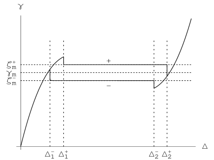
Figure 5: $\gamma-\Delta$ curves for the preferred solutions.

We can see that the curves shown in figure 5 capture some important features of the engineering $\gamma-\Delta$ curves measured in experiments (see Shaw $\&$ Kyriakides 1995, 1997; Sun et al. 2000; Tse $\&$ Sun 2000). For example, the stress peak (for the loading part) and stress valley (for the unloading part), the stress plateaus, the hysteresis loop and so on.

To draw figure 5, we just use the principle of minimizing the total pseudo-potential energy. We suppose that the configuration of the layer can jump from one metastable solution to another metastable/stable solution once the pseudo-potential energy of the latter one becomes smaller than the former one. But in fact, there may exist potential barriers between two metastable solutions. In this case, if we don’t give the layer enough perturbation, the layer will keep in its original metastable solution until this solution become unstable or some other limitation conditions happen. Thus, the curves shown in figure 5 are not necessarily the actual curves measured in the experiments, as metastable solutions may be maintained.

Alternatively, we can use the “limit-point” instability criterion for the onset of the nucleation or coalescence process. For the loading part, we assume that the layer keeps in the first constant solution until the total displacement $\Delta$ reaches $V_{0}$ (a “limit-point”; see figure 1), which corresponds to the peak stress value. As the total displacement goes on increasing, the martensite phase will nucleate even for the homogeneous deformation, thus the configuration of the layer jumps from the constant solution to the first non-trivial solution, i.e., the nucleation process happens. As $\Delta$ further increases, the deformation follows the first non-trivial solution. Once $\Delta$ reaches $\Delta_{4}^{+}$, another “limit-point” is also reached (see figure 1), the deformation of the layer jumps to the third constant solution. Thus, it is at the displacement value $\Delta=\Delta_{4}^{+}$ that coalescence process happens. Similarly, for the unloading part, we assume that the nucleation process happens at $\Delta=V_{1}$ (a “limit-point”) and the coalescence process happens at $\Delta=\Delta_{3}^{-}$ (another “limit-point”; see figure 2). The corresponding $\gamma-\Delta$ curves are shown in figure 6.

Figure 6: $\gamma-\Delta$ curves based on the “limit-point” criterion.

We can see that the curves shown in figure 6 are consistent with the experimental results (see Shaw $\&$ Kyriakides 1995, 1997; Sun et al. 2000; Tse $\&$ Sun 2000).

6 Analysis on the coalescence process

In this section, we shall give some analysis on the coalescence process, which plays a central role in the whole phase transition process. The following analysis of this section are based on the analytical solutions obtained in the section 5. Here we wish to give some descriptions and explanations for the origin of the instability during the coalescence process, the accompanying stress drop/jump and the morphology varies of the specimen. We shall also consider the size-effect of the specimens on the coalescence process.

As mentioned before, the coalescence process of phase fronts observed in quasi-static experiments is a dynamic one, which is an indication that an instability occurs. In subsection 5.2, we have already used the minimum energy principle to model the coalescence process (see figure 5). By comparing the total pseudo-potential energies of the constant solutions and nontrivial solutions, we found that the coalescence process should take place at the point $\Delta=\Delta_{2}^{+}$ for the loading case and $\Delta=\Delta_{1}^{-}$ for the unloading case. Besides the minimum energy principle, another possible reason for the onset of the coalescence process could be the fact that some “limit-points” have been reached. In subsection 5.2, we also used the “limit-points” instability criterion to model the coalescence process (see figure 6). We found that it was at the points $\Delta=\Delta_{4}^{+}$ for the loading case and $\Delta=\Delta_{3}^{-}$ for the unloading case that some “limit-points” had been reached and the coalescence process took place.

Remark: In the sequel, we shall only use the “limit-points” instability criterion to model the coalescence process.

Systematic experimental results have obviously shown that the coalescence process is inevitably accompanied the varies of the stress value and the surface morphology of the specimen. Here we shall use our model to describe these phenomena. For the purpose of clearness, we consider the second nontrivial solution (i.e., we choose $n=2$ in equation (5.18)) and consider the case that the phase fronts coalesce at the middle part of the layer. Thus the transformation scheme can be simply written as $MA+AM\rightarrow M$ for the loading case and $AM+MA\rightarrow A$ for the unloading case. Figure 7(a) shows the engineering stress-strain curve corresponding to the coalescence process during the loading case ($a=0.0043$). Corresponding to the 5 points $A$–$E$ show in figure 7(a), we plot the profiles of the layer in figure 7(b).

(a)

(b)

Figure 7: (a) Engineering stress-strain curve for the coalescence process during the loading case ($a=0.0043$). (b) Profiles of the layer corresponding to the 5 points $A$–$E$.

Here the radial deformation has been enlarged for clearness. From figure 7, we can see that the stress drop and the deformation process of the layer are very similar to the actual experimental procedures. Figure 8 shows the stress jump and the deformation process of the layer corresponding to the coalescence process during the unloading case ($a=0.0043$).

(a)

(b)

Figure 8: (a) Engineering stress-strain curve for the coalescence process during the unloading case ($a=0.0043$). (b) Profiles of the layer corresponding to the 5 points $A$–$E$.

We can see that the coalescence process shown in figure 8 is also consistent with the experimental results.

Next, we consider the influence of the geometric size effect of the layer on the coalescence process. From (5.15) and (5.18), we can see the nontrivial solutions obtained here depend directly on the half thickness-length ratio of the layer, which shows the fact that our model can reflect some important information on the geometric size effect. Here we only consider the loading case, and the similar result can also be derived for the unloading case. Figure 9 shows the $\gamma-\Delta$ curves of the second nontrivial solutions ($n=2$) corresponding to some different half thickness-length ratio.

Figure 9: $\gamma-\Delta$ curves of the second nontrivial solutions corresponding to some different half thickness-length ratio ($a=0.0026$, $0.0035$, $0.0043$).

From figure 9, we can see that as $a$ decreases, the $\gamma-\Delta$ curve of the non-trivial solution moves towards the constant solution. Actually, one can prove that the $\gamma-\Delta$ curve of the non-trivial solution moves toward first constant solution when $\xi_{m}^{+}<\gamma<\xi_{2}^{+}$ and towards the third constant solution when $\xi_{1}^{+}<\gamma<\xi_{m}^{+}$. The following is the proof for the case of the second nontrivial solutions ($n=2$) and $\xi_{1}^{+}<\gamma<\xi_{m}^{+}$ (the case of other nontrivial solutions and $\xi_{m}^{+}<\gamma<\xi_{2}^{+}$ can be proved similarly).

First, for the second nontrivial solution, we have the following equation (cf. (5.18))

$$\frac{1}{2}=a\int_{g_{1}^{+}}^{g_{2}^{+}}\sqrt{\frac{\frac{1}{6}-D_{3}V}{C^{+}+f^{+}(V)}}dV,\ \ \$$

which can be considered as a relationship between the half thickness-length ratio $a$ and the constant $C^{+}$. Through some simple analysis, we find that the equation $C^{+}+f^{+}(V)=0$ has four real roots $\alpha_{1}^{+}\leq g_{1}^{+}\leq g_{2}^{+}\leq\alpha_{2}^{+}$ if and only if

$$C_{2}^{+}\leq C^{+}\leq\textrm{min}(C_{1}^{+},C_{3}^{+}),\ \$$

where

$$C_{i}^{+}=-f_{i}^{+}(v_{i}^{+}),\ \ \ i=1,2,3.$$

In this case, the function $C^{+}+f^{+}(V)$ can be written in the following form

$$C^{+}+f^{+}(V)=f_{C}(V)(V-\alpha_{1}^{+})(V-g_{1}^{+})(V-g_{2}^{+})(V-\alpha_{2}^{+}),\ \$$

where $f_{C}(V)$ is a non-zero and bounded continuous function depending on the constant $C$.

Through some further analysis, we find that when $\xi_{1}^{+}<\gamma<\xi_{m}^{+}$, $C^{+}$ should satisfy $C_{2}^{+}\leq C^{+}\leq C_{3}^{+}$ and

$$\lim_{C^{+}\rightarrow C_{3}^{+}}\alpha_{1}^{+}<v_{1}^{+}<\lim_{C^{+}\rightarrow C_{3}^{+}}g_{1}^{+}<v_{2}^{+}<\lim_{C^{+}\rightarrow C_{3}^{+}}g_{2}^{+}=v_{3}^{+}=\lim_{C^{+}\rightarrow C_{3}^{+}}\alpha_{2}^{+},\ \$$

where $v_{1}^{+}$, $v_{2}^{+}$ and $v_{3}^{+}$ are the three real roots of equation (5.14). From (6.1) and (6.3), we have

$$a=\frac{1}{2\int_{g_{1}^{+}}^{g_{2}^{+}}\sqrt{\frac{1/6-D_{3}V}{f_{C}(V)(V-\alpha_{1}^{+})(V-g_{1}^{+})(V-g_{2}^{+})(V-\alpha_{2}^{+})}}dV}.\ \$$

Thus as $a$ tends to zero, the integration $\int_{g_{1}^{+}}^{g_{2}^{+}}\sqrt{\frac{1/6-D_{3}V}{f_{C}(V)(V-\alpha_{1}^{+})(V-g_{1}^{+})(V-g_{2}^{+})(V-\alpha_{2}^{+})}}dV$ should tends to infinity, and this is equivalent to $C^{+}$ tending to $C_{3}^{+}$. By using (5.15) and (6.5), we can give the following derivation

$$\Delta =\int_{0}^{1}VdZ=2\int_{0}^{\frac{1}{2}}VdZ=2\int_{g_{1}^{+}}^{g_{2}^{+}}V\frac{dZ}{dV}dV$$

$$=2a\int_{g_{1}^{+}}^{g_{2}^{+}}V\sqrt{\frac{1/6-D_{3}V}{f_{C}(V)(V-\alpha_{1}^{+})(V-g_{1}^{+})(V-g_{2}^{+})(V-\alpha_{2}^{+})}}dV$$

$$=\frac{\int_{g_{1}^{+}}^{g_{2}^{+}}V\sqrt{\frac{1/6-D_{3}V}{f_{C}(V)(V-\alpha_{1}^{+})(V-g_{1}^{+})(V-g_{2}^{+})(V-\alpha_{2}^{+})}}dV}{\int_{g_{1}^{+}}^{g_{2}^{+}}\sqrt{\frac{1/6-D_{3}V}{f_{C}(V)(V-\alpha_{1}^{+})(V-g_{1}^{+})(V-g_{2}^{+})(V-\alpha_{2}^{+})}}dV}$$

$$=g_{2}^{+}-\frac{\int_{g_{1}^{+}}^{g_{2}^{+}}(g_{2}^{+}-V)\sqrt{\frac{1/6-D_{3}V}{f_{C}(V)(V-\alpha_{1}^{+})(V-g_{1}^{+})(V-g_{2}^{+})(V-\alpha_{2}^{+})}}dV}{\int_{g_{1}^{+}}^{g_{2}^{+}}\sqrt{\frac{1/6-D_{3}V}{f_{C}(V)(V-\alpha_{1}^{+})(V-g_{1}^{+})(V-g_{2}^{+})(V-\alpha_{2}^{+})}}dV}$$

$$=g_{2}^{+}-\frac{\int_{g_{1}^{+}}^{g_{2}^{+}}\sqrt{\frac{(1/6-D_{3}V)(g_{2}^{+}-V)}{f_{C}(V)(V-\alpha_{1}^{+})(V-g_{1}^{+})(\alpha_{2}^{+}-V)}}dV}{\int_{g_{1}^{+}}^{g_{2}^{+}}\sqrt{\frac{1/6-D_{3}V}{f_{C}(V)(V-\alpha_{1}^{+})(V-g_{1}^{+})(V-g_{2}^{+})(V-\alpha_{2}^{+})}}dV}.$$

By using (6.4), it is easy to prove

$$\lim_{C\rightarrow C_{3}^{+}}\int_{g_{1}^{+}}^{g_{2}^{+}}\sqrt{\frac{(1/6-D_{3}V)(g_{2}^{+}-V)}{f_{C}(V)(V-\alpha_{1}^{+})(V-g_{1}^{+})(\alpha_{2}^{+}-V)}}dV<+\infty$$

and

$$\lim_{C\rightarrow C_{3}^{+}}\int_{g_{1}^{+}}^{g_{2}^{+}}\sqrt{\frac{1/6-D_{3}V}{f_{C}(V)(V-\alpha_{1}^{+})(V-g_{1}^{+})(V-g_{2}^{+})(V-\alpha_{2}^{+})}}dV=+\infty.$$

Thus, as $a$ tends to zero, the total elongation of the layer should satisfy

$$\lim_{a\rightarrow 0}\Delta=\lim_{C\rightarrow C_{3}^{+}}\Delta=\lim_{C\rightarrow C_{3}^{+}}g_{2}^{+}=v_{3}^{+}.\ \ \$$

This means that the $\gamma-\Delta$ curve of the second nontrivial solution tends to that of the third constant solution as $a$ tends to zero when $\xi_{1}^{+}<\gamma<\xi_{m}^{+}$.

Figure 9 shows that the $\gamma-\Delta$ curve of the nontrivial solution has a snap-back structure. But in a purely loading process, the total elongation $\Delta$ cannot decrease. Thus the state of the layer should jump from the nontrivial solution to the constant solution at some special point, which corresponds to the coalescence process. Here we also use the “limit-points” instability criterion to model the coalescence process. The actual $\gamma-\Delta$ curves of the coalescence processes corresponding to some different half thickness-length ratio are shown in figure 10.

Figure 10: Engineering stress-strain curves for the coalescence process during the loading case ($a=0.0026$, $0.0035$, $0.0043$).

From figure 10, we can see that as $a$ decreases, the stress drop during the coalescence process also decreases. Actually, (6.7) implies that the limit point should tend to the third constant solution as $a$ tends to zero. Thus, the stress drop should tend to zero as $a$ tends to zero. Similarly, in the process of AM+MA$\rightarrow$A during the unloading case, the stress jump should tend to zero as $a$ tends to zero. Thus we can say that the geometrical size of the specimen plays an important role in the coalescence process.

7 Conclusions

In this paper, we aim to study the phase fronts coalescence phenomena during the phase transition process in a thin SMA layer. For that purpose, we derived a quasi-2D model with a non-convex effective strain energy function while taking into account the rate-independent dissipation effect.

In a two-dimensional setting, we studied the symmetric deformation of a thin SMA layer. Based on the field equations and the traction-free boundary conditions, by using the coupled series-asymptotic expansion method, we expressed the total elastic potential energy of the layer $\Phi_{E}$ as a function of the leading order term of the axial strain $V(X)$. We further considered the mechanical dissipation effect in a purely one-dimensional setting and expressed the total amount of mechanical dissipations $\Phi_{D}^{+}$ (loading case) and $\Phi_{D}^{-}$ (unloading case) as functions of the axial strain $V(X)$. The equilibrium equation was then determined by using the principle of maximizing the total energy dissipation. We further considered an illustrative example with some given material constants and some special form of dissipation density functions. With the free end boundary conditions, we managed to construct the analytical solutions for both a force-controlled problem and a displacement-controlled problem.

Based on the analytical solutions obtained and by using the limit-point instability criterion, we studied the phase fronts coalescence phenomena. It was revealed that during the coalescence process, the configurations of the layer switched from the nontrivial solution modes to the trivial solution modes, which was caused by the presence of the “limit points”. The morphology varies of the layer and the accompanying stress drop/jump during the coalescence process can be described. The influence of the thickness-length ratio of the specimen on the coalescence process was also studied. It was found that the zero limit of the thickness-length ratio can lead to the smooth switch of nontrivial modes to trivial modes with no stress drop or stress jump.

Appendix A Incremental elastic moduli

For initially isotropic material, in the case that there are no prestresses, the elastic potential energy function $\Psi$ should be a function of the principal stretches $\lambda_{1}$ and $\lambda_{2}$, namely $\Psi$=$\Psi(\lambda_{1},\lambda_{2})$. Denote by $\Psi_{j}=\frac{\partial\Psi}{\partial\lambda_{j}}|_{\lambda_{1}=\lambda_{2}=1}$, then $\Psi_{1}=\Psi_{2}$ should vanish since there are no prestresses.

The non-zero first order incremental elastic moduli can be written as

$$\tau_{1}=a^{1}_{1111}=\Psi_{11},$$

$$\tau_{2}=a^{1}_{1122}=\Psi_{12},$$

$$\tau_{3}=a^{1}_{1212}=\frac{1}{2}(\tau_{1}-\tau_{2}),$$

$$\tau_{4}=a^{1}_{1221}=\tau_{3}.$$

There are only two independent constants among $\tau_{i}$.

The non-zero second order incremental elastic moduli can be written as

$$\eta_{1}=a^{2}_{111111}=\Psi_{111},$$

$$\eta_{2}=a^{2}_{111122}=\Psi_{112},$$

$$\eta_{3}=a^{2}_{111212}=\frac{1}{4}(\tau_{1}+\tau_{2}+\eta_{1}-\eta_{2}),$$

$$\eta_{4}=a^{2}_{111221}=\frac{1}{4}(-\tau_{1}-\tau_{2}+\eta_{1}-\eta_{2}),$$

There are only two additional independent constants among $\eta_{i}$.

The non-zero third order incremental elastic moduli can be written as

$$\theta_{1}=a^{3}_{11111111}=\Psi_{1111},$$

$$\theta_{2}=a^{3}_{11111122}=\Psi_{1112},$$

$$\theta_{3}=a^{3}_{11111212}=\frac{1}{12}(-3\tau_{1}-3\tau_{2}+3\eta_{1}+3\eta_{2}+2\theta_{1}-2\theta_{2}),$$

$$\theta_{4}=a^{3}_{11111221}=\frac{1}{12}(3\tau_{1}+3\tau_{2}-3\eta_{1}-3\eta_{2}+2\theta_{1}-2\theta_{2}),$$

$$\theta_{5}=a^{3}_{11112222}=\Psi_{1122},$$

$$\theta_{6}=a^{3}_{11121222}=\frac{1}{12}(-3\tau_{1}-3\tau_{2}+6\eta_{2}+\theta_{1}+2\theta_{2}-3\theta_{5}),$$

$$\theta_{7}=a^{3}_{11122122}=\frac{1}{12}(3\tau_{1}+3\tau_{2}-6\eta_{2}+\theta_{1}+2\theta_{2}-3\theta_{5}),$$

$$\theta_{8}=a^{3}_{12121212}=\frac{1}{8}(3\tau_{1}+3\tau_{2}+6\eta_{1}-6\eta_{2}+\theta_{1}-4\theta_{2}+3\theta_{5}),$$

$$\theta_{9}=a^{3}_{12121221}=\frac{1}{8}(-3\tau_{1}-3\tau_{2}+\theta_{1}-4\theta_{2}+3\theta_{5}),$$

$$\theta_{10}=a^{3}_{12122121}=\frac{1}{8}(3\tau_{1}+3\tau_{2}-2\eta_{1}+2\eta_{2}+\theta_{1}-4\theta_{2}+3\theta_{5}),$$

There are only three additional independent constants among $\theta_{i}$.

Appendix B Non-dimensional field equations

The full forms of the non-dimensional field equations (3.15) and (3.16) are given by:

$${2{\tau_{3}}u_{s}+({\tau_{2}}+{\tau_{3}})w_{x}+s(4{\tau_{3}}u_{ss}+(2{\tau_{2}}+2{\tau_{3}})w_{xs})+{\tau_{1}}u_{xx}+\epsilon(2{\eta_{3}}wu_{s}+2{\eta_{3}}u_{s}u_{x}}$$

$${+({\eta_{2}}+{\eta_{4}})ww_{x}+({\eta_{2}}+{\eta_{4}})u_{x}w_{x}+s^{2}(8{\eta_{3}}w_{s}u_{ss}+8{\eta_{3}}u_{s}w_{ss}+4{\eta_{4}}w_{ss}w_{x}}$$

$${+(4{\eta_{2}}+4{\eta_{4}})w_{s}w_{xs})+{\eta_{2}}wu_{xx}+{\eta_{1}}u_{x}u_{xx}+s(16{\eta_{3}}u_{s}w_{s}+4{\eta_{3}}wu_{ss}+4{\eta_{3}}u_{ss}u_{x}}$$

$${+(2{\eta_{2}}+8{\eta_{4}})w_{s}w_{x}+8{\eta_{3}}u_{s}u_{xs}+4{\eta_{4}}w_{x}u_{xs}+(2{\eta_{2}}+2{\eta_{4}})ww_{xs}+(2{\eta_{2}}+2{\eta_{4}})u_{x}w_{xs}}$$

$${+2{\eta_{2}}w_{s}u_{xx}+2{\eta_{4}}u_{s}w_{xx}+{\eta_{3}}w_{x}w_{xx}))+\epsilon^{2}(\theta_{3}w^{2}u_{s}+2\theta_{6}wu_{s}u_{x}+\theta_{3}u_{s}u_{x}^{2}}$$

$$+(\frac{\theta_{2}}{2}+\frac{\theta_{4}}{2})w^{2}w_{x}+(\theta_{5}+\theta_{7})wu_{x}w_{x}+(\frac{\theta_{2}}{2}+\frac{\theta_{4}}{2})u_{x}^{2}w_{x}+s^{3}(8\theta_{3}w_{s}^{2}u_{ss}$$

$$+16\theta_{3}u_{s}w_{s}w_{ss}+8\theta_{4}w_{s}w_{ss}w_{x}+(4\theta_{2}+4\theta_{4})w_{s}^{2}w_{xs})+\frac{1}{2}\theta_{5}w^{2}u_{xx}+\theta_{2}wu_{x}u_{xx}$$

$$+\frac{1}{2}\theta_{1}u_{x}^{2}u_{xx}+s^{2}(28\theta_{3}u_{s}w_{s}^{2}+8\theta_{8}u_{s}^{2}u_{ss}+8\theta_{3}ww_{s}u_{ss}+8\theta_{3}wu_{s}w_{ss}+8\theta_{6}w_{s}u_{ss}u_{x}$$

$$+8\theta_{6}u_{s}w_{ss}u_{x}+(2\theta_{2}+14\theta_{4})w_{s}^{2}w_{x}+8\theta_{9}u_{s}u_{ss}w_{x}+4\theta_{4}ww_{ss}w_{x}+4\theta_{7}w_{ss}u_{x}w_{x}$$

$$+2\theta_{10}u_{ss}w_{x}^{2}+16\theta_{6}u_{s}w_{s}u_{xs}+8\theta_{7}w_{s}w_{x}u_{xs}+(4\theta_{6}+4\theta_{9})u_{s}^{2}w_{xs}+(4\theta_{2}+4\theta_{4})ww_{s}w_{xs}$$

$$+(4\theta_{5}+4\theta_{7})w_{s}u_{x}w_{xs}+(4\theta_{10}+4\theta_{7})u_{s}w_{x}w_{xs}+(\theta_{6}+\theta_{9})w_{x}^{2}w_{xs}+2\theta_{5}w_{s}^{2}u_{xx}$$

$$+4\theta_{7}u_{s}w_{s}w_{xx}+2\theta_{6}w_{s}w_{x}w_{xx})+s(4\theta_{8}u_{s}^{3}+16\theta_{3}wu_{s}w_{s}+2\theta_{3}w^{2}u_{ss}+16\theta_{6}u_{s}w_{s}u_{x}$$

$$+4\theta_{6}wu_{ss}u_{x}+2\theta_{3}u_{ss}u_{x}^{2}+(2\theta_{6}+6\theta_{9})u_{s}^{2}w_{x}+(2\theta_{2}+8\theta_{4})ww_{s}w_{x}+(3\theta_{10}+2\theta_{7})u_{s}w_{x}^{2}$$

$$+(2\theta_{5}+8\theta_{7})w_{s}u_{x}w_{x}+(\frac{\theta_{6}}{2}+\frac{\theta_{9}}{2})w_{x}^{3}+8\theta_{6}wu_{s}u_{xs}+8\theta_{3}u_{s}u_{x}u_{xs}+4\theta_{7}ww_{x}u_{xs}$$

$$+4\theta_{4}u_{x}w_{x}u_{xs}+(\theta_{2}+\theta_{4})w^{2}w_{xs}+(2\theta_{5}+2\theta_{7})wu_{x}w_{xs}+(\theta_{2}+\theta_{4})u_{x}^{2}w_{xs}+2\theta_{3}u_{s}^{2}u_{xx}$$

$$+2\theta_{5}ww_{s}u_{xx}+2\theta_{2}w_{s}u_{x}u_{xx}+2\theta_{4}u_{s}w_{x}u_{xx}+\frac{1}{2}\theta_{3}w_{x}^{2}u_{xx}+2\theta_{7}wu_{s}w_{xx}+2\theta_{4}u_{s}u_{x}w_{xx}$$

$$+\theta_{6}ww_{x}w_{xx}+\theta_{3}u_{x}w_{x}w_{xx}))=0,$$

$$6\tau_{1}w_{s}+(2\tau_{2}+2\tau_{3})u_{xs}+\tau_{3}w_{xx}+4s\tau_{1}w_{ss}+\epsilon({4{\eta_{3}}u_{s}^{2}+6{\eta_{1}}ww_{s}}$$

$${+8s^{2}{\eta_{1}}w_{s}w_{ss}+6{\eta_{2}}w_{s}u_{x}+6{\eta_{4}}u_{s}w_{x}+2{\eta_{3}}w_{x}^{2}+(2{\eta_{2}}+2{\eta_{4}})wu_{xs}}$$

$${+(2{\eta_{2}}+2{\eta_{4}})u_{x}u_{xs}+2{\eta_{4}}u_{s}u_{xx}+{\eta_{3}}w_{x}u_{xx}+{\eta_{3}}ww_{xx}+{\eta_{3}}u_{x}w_{xx}}$$

$${+s(12{\eta_{1}}w_{s}^{2}+8{\eta_{3}}u_{s}u_{ss}+4{\eta_{1}}ww_{ss}+4{\eta_{2}}w_{ss}u_{x}+4{\eta_{4}}u_{ss}w_{x}}$$

$${+(4{\eta_{2}}+4{\eta_{4}})w_{s}u_{xs}+8{\eta_{4}}u_{s}w_{xs}+4{\eta_{3}}w_{x}w_{xs}+2{\eta_{3}}w_{s}w_{xx})})$$

$$+\epsilon^{2}({4{\theta_{3}}wu_{s}^{2}+3{\theta_{1}}w^{2}w_{s}+8s^{3}{\theta_{1}}w_{s}^{2}w_{ss}+4{\theta_{6}}u_{s}^{2}u_{x}+6{\theta_{2}}ww_{s}u_{x}+3{\theta_{5}}w_{s}u_{x}^{2}}$$

$${+6{\theta_{4}}wu_{s}w_{x}+6{\theta_{7}}u_{s}u_{x}w_{x}+2{\theta_{3}}ww_{x}^{2}+2{\theta_{6}}u_{x}w_{x}^{2}+({\theta_{2}}+{\theta_{4}})w^{2}u_{xs}}$$

$${+(2{\theta_{5}}+2{\theta_{7}})wu_{x}u_{xs}+({\theta_{2}}+{\theta_{4}})u_{x}^{2}u_{xs}+2{\theta_{7}}wu_{s}u_{xx}+2{\theta_{4}}u_{s}u_{x}u_{xx}}$$

$${+{\theta_{6}}ww_{x}u_{xx}+{\theta_{3}}u_{x}w_{x}u_{xx}+\frac{1}{2}{\theta_{3}}w^{2}w_{xx}+{\theta_{6}}wu_{x}w_{xx}+\frac{1}{2}{\theta_{3}}u_{x}^{2}w_{xx}}$$

$${+s^{2}(12{\theta_{1}}w_{s}^{3}+16{\theta_{3}}u_{s}w_{s}u_{ss}+8{\theta_{3}}u_{s}^{2}w_{ss}+8{\theta_{1}}ww_{s}w_{ss}+8{\theta_{2}}w_{s}w_{ss}u_{x}}$$

$${+8{\theta_{4}}w_{s}u_{ss}w_{x}+8{\theta_{4}}u_{s}w_{ss}w_{x}+2{\theta_{3}}w_{ss}w_{x}^{2}+(4{\theta_{2}}+4{\theta_{4}})w_{s}^{2}u_{xs}}$$

$${+16{\theta_{4}}u_{s}w_{s}w_{xs}+8{\theta_{3}}w_{s}w_{x}w_{xs}+2{\theta_{3}}w_{s}^{2}w_{xx})+s(20{\theta_{3}}u_{s}^{2}w_{s}+12{\theta_{1}}ww_{s}^{2}}$$

$${+8{\theta_{3}}wu_{s}u_{ss}+2{\theta_{1}}w^{2}w_{ss}+12{\theta_{2}}w_{s}^{2}u_{x}+8{\theta_{6}}u_{s}u_{ss}u_{x}+4{\theta_{2}}ww_{ss}u_{x}}$$

$${+2{\theta_{5}}w_{ss}u_{x}^{2}+24{\theta_{4}}u_{s}w_{s}w_{x}+4{\theta_{4}}wu_{ss}w_{x}+4{\theta_{7}}u_{ss}u_{x}w_{x}+7{\theta_{3}}w_{s}w_{x}^{2}}$$

$${+(4{\theta_{6}}+4{\theta_{9}})u_{s}^{2}u_{xs}+(4{\theta_{2}}+4{\theta_{4}})ww_{s}u_{xs}+(4{\theta_{5}}+4{\theta_{7}})w_{s}u_{x}u_{xs}+}$$

$${(4{\theta_{10}}+4{\theta_{7}})u_{s}w_{x}u_{xs}+({\theta_{6}}+{\theta_{9}})w_{x}^{2}u_{xs}+8{\theta_{4}}wu_{s}w_{xs}+8{\theta_{7}}u_{s}u_{x}w_{xs}}$$

$${+4{\theta_{3}}ww_{x}w_{xs}+4{\theta_{6}}u_{x}w_{x}w_{xs}+4{\theta_{7}}u_{s}w_{s}u_{xx}+2{\theta_{6}}w_{s}w_{x}u_{xx}+2{\theta_{1}0}u_{s}^{2}w_{xx}}$$

$${+2{\theta_{3}}ww_{s}w_{xx}+2{\theta_{6}}w_{s}u_{x}w_{xx}+2{\theta_{9}}u_{s}w_{x}w_{xx}+\frac{1}{2}{\theta_{8}}w_{x}^{2}w_{xx})})=0.$$

Appendix C

The formulas of the constants $a_{i}$ ($i=1,\cdots,25$) in (3.26)-(3.28) are given below:

$${{a_{1}}=-\frac{{\eta_{2}}}{2{\tau_{3}}}+\frac{{\tau_{2}}{\eta_{3}}}{2{{{\tau_{3}}}^{2}}}+\frac{{\eta_{3}}}{2{\tau_{3}}}-\frac{{\eta_{4}}}{2{\tau_{3}}},}$$

$${{a_{2}}=-\frac{{\eta_{2}}}{2{\tau_{3}}}+\frac{{\tau_{2}}{\eta_{3}}}{2{{{\tau_{3}}}^{2}}}+\frac{{\eta_{3}}}{2{\tau_{3}}}-\frac{{\eta_{4}}}{2{\tau_{3}}},}$$

$${{a_{3}}=-\frac{{\eta_{2}}}{2{\tau_{3}}}+\frac{{\tau_{1}}{\eta_{3}}}{2{{{\tau_{3}}}^{2}}},}$$

$${{a_{4}}=-\frac{{\eta_{1}}}{2{\tau_{3}}}+\frac{{\tau_{1}}{\eta_{3}}}{2{{{\tau_{3}}}^{2}}},}$$

$${{a_{5}}=\frac{{\eta_{2}}{\eta_{3}}}{2{{{\tau_{3}}}^{2}}}-\frac{{\tau_{2}}{{{\eta_{3}}}^{2}}}{2{{{\tau_{3}}}^{3}}}-\frac{{{{\eta_{3}}}^{2}}}{2{{{\tau_{3}}}^{2}}}+\frac{{\eta_{3}}{\eta_{4}}}{2{{{\tau_{3}}}^{2}}}-\frac{{\theta_{2}}}{4{\tau_{3}}}+\frac{{\tau_{2}}{\theta_{3}}}{4{{{\tau_{3}}}^{2}}}+\frac{{\theta_{3}}}{4{\tau_{3}}}-\frac{{\theta_{4}}}{4{\tau_{3}}},}$$

$${{a_{6}}=\frac{{\eta_{2}}{\eta_{3}}}{{{{\tau_{3}}}^{2}}}-\frac{{\tau_{2}}{{{\eta_{3}}}^{2}}}{{{{\tau_{3}}}^{3}}}-\frac{{{{\eta_{3}}}^{2}}}{{{{\tau_{3}}}^{2}}}+\frac{{\eta_{3}}{\eta_{4}}}{{{{\tau_{3}}}^{2}}}-\frac{{\theta_{5}}}{2{\tau_{3}}}+\frac{{\tau_{2}}{\theta_{6}}}{2{{{\tau_{3}}}^{2}}}+\frac{{\theta_{6}}}{2{\tau_{3}}}-\frac{{\theta_{7}}}{2{\tau_{3}}},}$$

$${{a_{7}}=\frac{{\eta_{2}}{\eta_{3}}}{2{{{\tau_{3}}}^{2}}}-\frac{{\tau_{2}}{{{\eta_{3}}}^{2}}}{2{{{\tau_{3}}}^{3}}}-\frac{{{{\eta_{3}}}^{2}}}{2{{{\tau_{3}}}^{2}}}+\frac{{\eta_{3}}{\eta_{4}}}{2{{{\tau_{3}}}^{2}}}-\frac{{\theta_{2}}}{4{\tau_{3}}}+\frac{{\tau_{2}}{\theta_{3}}}{4{{{\tau_{3}}}^{2}}}+\frac{{\theta_{3}}}{4{\tau_{3}}}-\frac{{\theta_{4}}}{4{\tau_{3}}},}$$

$${{a_{8}}=\frac{{\eta_{2}}{\eta_{3}}}{2{{{\tau_{3}}}^{2}}}-\frac{{\tau_{1}}{{{\eta_{3}}}^{2}}}{2{{{\tau_{3}}}^{3}}}+\frac{{\tau_{1}}{\theta_{3}}}{4{{{\tau_{3}}}^{2}}}-\frac{{\theta_{5}}}{4{\tau_{3}}},}$$

$${{a_{9}}=\frac{{\eta_{1}}{\eta_{3}}}{2{{{\tau_{3}}}^{2}}}+\frac{{\eta_{2}}{\eta_{3}}}{2{{{\tau_{3}}}^{2}}}-\frac{{\tau_{1}}{{{\eta_{3}}}^{2}}}{{{{\tau_{3}}}^{3}}}-\frac{{\theta_{2}}}{2{\tau_{3}}}+\frac{{\tau_{1}}{\theta_{6}}}{2{{{\tau_{3}}}^{2}}},}$$

$${{a_{10}}=\frac{{\eta_{1}}{\eta_{3}}}{2{{{\tau_{3}}}^{2}}}-\frac{{\tau_{1}}{{{\eta_{3}}}^{2}}}{2{{{\tau_{3}}}^{3}}}-\frac{{\theta_{1}}}{4{\tau_{3}}}+\frac{{\tau_{1}}{\theta_{3}}}{4{{{\tau_{3}}}^{2}}},}$$

$${{a_{11}}=\frac{{\eta_{2}}}{6{\tau_{1}}}+\frac{{\tau_{2}}{\eta_{2}}}{6{\tau_{1}}{\tau_{3}}}-\frac{2{\eta_{3}}}{3{\tau_{1}}}-\frac{{{{\tau_{2}}}^{2}}{\eta_{3}}}{3{\tau_{1}}{{{\tau_{3}}}^{2}}}-\frac{2{\tau_{2}}{\eta_{3}}}{3{\tau_{1}}{\tau_{3}}}+\frac{2{\eta_{4}}}{3{\tau_{1}}}+\frac{2{\tau_{2}}{\eta_{4}}}{3{\tau_{1}}{\tau_{3}}},}$$

$${{a_{12}}=\frac{{\eta_{2}}}{3{\tau_{1}}}+\frac{{\tau_{2}}{\eta_{2}}}{3{\tau_{1}}{\tau_{3}}}-\frac{{\eta_{3}}}{3{\tau_{1}}}-\frac{{\tau_{2}}{\eta_{3}}}{2{{{\tau_{3}}}^{2}}}-\frac{{{{\tau_{2}}}^{2}}{\eta_{3}}}{6{\tau_{1}}{{{\tau_{3}}}^{2}}}-\frac{{\eta_{3}}}{2{\tau_{3}}}-\frac{{\tau_{2}}{\eta_{3}}}{3{\tau_{1}}{\tau_{3}}}+\frac{{\eta_{4}}}{3{\tau_{1}}}+\frac{{\eta_{4}}}{2{\tau_{3}}}+\frac{{\tau_{2}}{\eta_{4}}}{3{\tau_{1}}{\tau_{3}}},}$$

$${{a_{13}}=\frac{{\eta_{1}}}{6{\tau_{1}}}+\frac{{\tau_{2}}{\eta_{1}}}{6{\tau_{1}}{\tau_{3}}}-\frac{{\tau_{1}}{\eta_{3}}}{6{{{\tau_{3}}}^{2}}}-\frac{{\tau_{2}}{\eta_{3}}}{6{{{\tau_{3}}}^{2}}}-\frac{{\eta_{3}}}{6{\tau_{3}}}+\frac{{\eta_{4}}}{6{\tau_{3}}},}$$

$${{a_{14}}=-\frac{{\tau_{2}}{\eta_{1}}}{3{{{\tau_{1}}}^{2}}}-\frac{{{{\tau_{2}}}^{2}}{\eta_{1}}}{6{{{\tau_{1}}}^{2}}{\tau_{3}}}+\frac{{\eta_{2}}}{3{\tau_{1}}}+\frac{{\tau_{2}}{\eta_{2}}}{3{\tau_{1}}{\tau_{3}}}-\frac{{\eta_{3}}}{3{\tau_{1}}}-\frac{{{{\tau_{2}}}^{2}}{\eta_{3}}}{6{\tau_{1}}{{{\tau_{3}}}^{2}}}-\frac{{\tau_{2}}{\eta_{3}}}{3{\tau_{1}}{\tau_{3}}}+\frac{{\eta_{4}}}{3{\tau_{1}}}+\frac{{\tau_{2}}{\eta_{4}}}{3{\tau_{1}}{\tau_{3}}},}$$

$${{a_{15}}=\frac{{\eta_{2}}}{3{\tau_{1}}}-\frac{{\tau_{2}}{\eta_{2}}}{3{{{\tau_{1}}}^{2}}}+\frac{{\tau_{2}}{\eta_{2}}}{3{\tau_{1}}{\tau_{3}}}-\frac{{{{\tau_{2}}}^{2}}{\eta_{2}}}{6{{{\tau_{1}}}^{2}}{\tau_{3}}}-\frac{{\eta_{3}}}{3{\tau_{1}}}-\frac{{{{\tau_{2}}}^{2}}{\eta_{3}}}{6{\tau_{1}}{{{\tau_{3}}}^{2}}}-\frac{{\tau_{2}}{\eta_{3}}}{3{\tau_{1}}{\tau_{3}}}+\frac{{\eta_{4}}}{3{\tau_{1}}}+\frac{{\tau_{2}}{\eta_{4}}}{3{\tau_{1}}{\tau_{3}}},}$$

$${{a_{16}}=-\frac{{\eta_{1}}}{6{\tau_{1}}}-\frac{{\tau_{2}}{\eta_{1}}}{6{\tau_{1}}{\tau_{3}}}+\frac{{\eta_{2}}}{6{\tau_{1}}}+\frac{{\eta_{2}}}{6{\tau_{3}}}+\frac{{\tau_{2}}{\eta_{2}}}{6{\tau_{1}}{\tau_{3}}}-\frac{{\tau_{2}}{\eta_{3}}}{6{{{\tau_{3}}}^{2}}}-\frac{{\eta_{3}}}{6{\tau_{3}}}+\frac{{\eta_{4}}}{6{\tau_{3}}},}$$

$${{a_{17}}=\frac{{\eta_{1}}}{6{\tau_{1}}}+\frac{{\tau_{2}}{\eta_{1}}}{6{\tau_{1}}{\tau_{3}}}-\frac{{\eta_{2}}}{6{\tau_{1}}}+\frac{{\eta_{2}}}{6{\tau_{3}}}-\frac{{\tau_{2}}{\eta_{2}}}{6{\tau_{1}}{\tau_{3}}}-\frac{{\tau_{2}}{\eta_{3}}}{6{{{\tau_{3}}}^{2}}}-\frac{{\eta_{3}}}{6{\tau_{3}}}+\frac{{\eta_{4}}}{6{\tau_{3}}},}$$

$${a_{18}}= \frac{{\tau_{2}}{\eta_{1}}}{12{{{\tau_{1}}}^{2}}}+\frac{{{{\tau_{2}}}^{3}}{\eta_{1}}}{24{{{\tau_{1}}}^{2}}{{{\tau_{3}}}^{2}}}+\frac{{{{\tau_{2}}}^{2}}{\eta_{1}}}{8{{{\tau_{1}}}^{2}}{\tau_{3}}}-\frac{{\eta_{2}}}{6{\tau_{1}}}+\frac{{\tau_{1}}{\eta_{2}}}{8{{{\tau_{3}}}^{2}}}+\frac{{\tau_{2}}{\eta_{2}}}{24{{{\tau_{3}}}^{2}}}-\frac{5{{{\tau_{2}}}^{2}}{\eta_{2}}}{24{\tau_{1}}{{{\tau_{3}}}^{2}}}+\frac{{\eta_{2}}}{24{\tau_{3}}}$$

$$-\frac{5{\tau_{2}}{\eta_{2}}}{12{\tau_{1}}{\tau_{3}}}+\frac{5{\eta_{3}}}{12{\tau_{1}}}-\frac{{\tau_{1}}{\tau_{2}}{\eta_{3}}}{8{{{\tau_{3}}}^{3}}}-\frac{5{{{\tau_{2}}}^{2}}{\eta_{3}}}{24{{{\tau_{3}}}^{3}}}+\frac{{{{\tau_{2}}}^{3}}{\eta_{3}}}{3{\tau_{1}}{{{\tau_{3}}}^{3}}}-\frac{{\tau_{1}}{\eta_{3}}}{8{{{\tau_{3}}}^{2}}}-\frac{5{\tau_{2}}{\eta_{3}}}{12{{{\tau_{3}}}^{2}}}+\frac{{{{\tau_{2}}}^{2}}{\eta_{3}}}{{\tau_{1}}{{{\tau_{3}}}^{2}}}$$

$$-\frac{7{\eta_{3}}}{24{\tau_{3}}}+\frac{13{\tau_{2}}{\eta_{3}}}{12{\tau_{1}}{\tau_{3}}}-\frac{5{\eta_{4}}}{12{\tau_{1}}}+\frac{{\tau_{1}}{\eta_{4}}}{8{{{\tau_{3}}}^{2}}}+\frac{7{\tau_{2}}{\eta_{4}}}{24{{{\tau_{3}}}^{2}}}-\frac{13{{{\tau_{2}}}^{2}}{\eta_{4}}}{24{\tau_{1}}{{{\tau_{3}}}^{2}}}+\frac{7{\eta_{4}}}{24{\tau_{3}}}-\frac{13{\tau_{2}}{\eta_{4}}}{12{\tau_{1}}{\tau_{3}}},$$

$${a_{19}}= \frac{{\tau_{2}}{\eta_{1}}}{24{{{\tau_{3}}}^{2}}}+\frac{{\eta_{1}}}{24{\tau_{3}}}-\frac{{\eta_{2}}}{6{\tau_{1}}}+\frac{{\tau_{2}}{\eta_{2}}}{12{{{\tau_{1}}}^{2}}}+\frac{{\tau_{1}}{\eta_{2}}}{8{{{\tau_{3}}}^{2}}}-\frac{5{{{\tau_{2}}}^{2}}{\eta_{2}}}{24{\tau_{1}}{{{\tau_{3}}}^{2}}}+\frac{{{{\tau_{2}}}^{3}}{\eta_{2}}}{24{{{\tau_{1}}}^{2}}{{{\tau_{3}}}^{2}}}-\frac{5{\tau_{2}}{\eta_{2}}}{12{\tau_{1}}{\tau_{3}}}$$

$$+\frac{{{{\tau_{2}}}^{2}}{\eta_{2}}}{8{{{\tau_{1}}}^{2}}{\tau_{3}}}+\frac{{\eta_{3}}}{6{\tau_{1}}}-\frac{{{{\tau_{1}}}^{2}}{\eta_{3}}}{24{{{\tau_{3}}}^{3}}}-\frac{7{\tau_{1}}{\tau_{2}}{\eta_{3}}}{24{{{\tau_{3}}}^{3}}}+\frac{{{{\tau_{2}}}^{2}}{\eta_{3}}}{4{{{\tau_{3}}}^{3}}}+\frac{{{{\tau_{2}}}^{3}}{\eta_{3}}}{12{\tau_{1}}{{{\tau_{3}}}^{3}}}-\frac{7{\tau_{1}}{\eta_{3}}}{24{{{\tau_{3}}}^{2}}}+\frac{{\tau_{2}}{\eta_{3}}}{2{{{\tau_{3}}}^{2}}}$$

$$+\frac{{{{\tau_{2}}}^{2}}{\eta_{3}}}{4{\tau_{1}}{{{\tau_{3}}}^{2}}}+\frac{{\eta_{3}}}{8{\tau_{3}}}+\frac{{\tau_{2}}{\eta_{3}}}{3{\tau_{1}}{\tau_{3}}}-\frac{{\eta_{4}}}{6{\tau_{1}}}+\frac{{\tau_{1}}{\eta_{4}}}{6{{{\tau_{3}}}^{2}}}-\frac{{\tau_{2}}{\eta_{4}}}{8{{{\tau_{3}}}^{2}}}-\frac{{{{\tau_{2}}}^{2}}{\eta_{4}}}{6{\tau_{1}}{{{\tau_{3}}}^{2}}}-\frac{{\eta_{4}}}{8{\tau_{3}}}-\frac{{\tau_{2}}{\eta_{4}}}{3{\tau_{1}}{\tau_{3}}},$$

$${a_{20}}= \frac{{\eta_{1}}}{24{\tau_{1}}}+\frac{{{{\tau_{2}}}^{2}}{\eta_{1}}}{24{\tau_{1}}{{{\tau_{3}}}^{2}}}+\frac{{\tau_{2}}{\eta_{1}}}{12{\tau_{1}}{\tau_{3}}}-\frac{{\eta_{2}}}{8{\tau_{1}}}+\frac{{\tau_{1}}{\eta_{2}}}{6{{{\tau_{3}}}^{2}}}-\frac{{\tau_{2}}{\eta_{2}}}{12{{{\tau_{3}}}^{2}}}-\frac{{{{\tau_{2}}}^{2}}{\eta_{2}}}{8{\tau_{1}}{{{\tau_{3}}}^{2}}}-\frac{{\eta_{2}}}{12{\tau_{3}}}-\frac{{\tau_{2}}{\eta_{2}}}{4{\tau_{1}}{\tau_{3}}}$$

$$+\frac{{\eta_{3}}}{12{\tau_{1}}}-\frac{{{{\tau_{1}}}^{2}}{\eta_{3}}}{12{{{\tau_{3}}}^{3}}}-\frac{{\tau_{1}}{\tau_{2}}{\eta_{3}}}{4{{{\tau_{3}}}^{3}}}+\frac{7{{{\tau_{2}}}^{2}}{\eta_{3}}}{24{{{\tau_{3}}}^{3}}}+\frac{{{{\tau_{2}}}^{3}}{\eta_{3}}}{24{\tau_{1}}{{{\tau_{3}}}^{3}}}-\frac{{\tau_{1}}{\eta_{3}}}{4{{{\tau_{3}}}^{2}}}+\frac{7{\tau_{2}}{\eta_{3}}}{12{{{\tau_{3}}}^{2}}}+\frac{{{{\tau_{2}}}^{2}}{\eta_{3}}}{8{\tau_{1}}{{{\tau_{3}}}^{2}}}$$

$$+\frac{7{\eta_{3}}}{24{\tau_{3}}}+\frac{{\tau_{2}}{\eta_{3}}}{6{\tau_{1}}{\tau_{3}}}-\frac{{\eta_{4}}}{12{\tau_{1}}}+\frac{{\tau_{1}}{\eta_{4}}}{4{{{\tau_{3}}}^{2}}}-\frac{7{\tau_{2}}{\eta_{4}}}{24{{{\tau_{3}}}^{2}}}-\frac{{{{\tau_{2}}}^{2}}{\eta_{4}}}{12{\tau_{1}}{{{\tau_{3}}}^{2}}}-\frac{7{\eta_{4}}}{24{\tau_{3}}}-\frac{{\tau_{2}}{\eta_{4}}}{6{\tau_{1}}{\tau_{3}}},$$

$${a_{21}}= -\frac{{\eta_{1}}}{8{\tau_{1}}}+\frac{{\tau_{1}}{\eta_{1}}}{6{{{\tau_{3}}}^{2}}}-\frac{{{{\tau_{2}}}^{2}}{\eta_{1}}}{8{\tau_{1}}{{{\tau_{3}}}^{2}}}-\frac{{\tau_{2}}{\eta_{1}}}{4{\tau_{1}}{\tau_{3}}}+\frac{{\eta_{2}}}{24{\tau_{1}}}-\frac{{\tau_{2}}{\eta_{2}}}{12{{{\tau_{3}}}^{2}}}+\frac{{{{\tau_{2}}}^{2}}{\eta_{2}}}{24{\tau_{1}}{{{\tau_{3}}}^{2}}}-\frac{{\eta_{2}}}{12{\tau_{3}}}+\frac{{\tau_{2}}{\eta_{2}}}{12{\tau_{1}}{\tau_{3}}}$$

$$-\frac{{{{\tau_{1}}}^{2}}{\eta_{3}}}{3{{{\tau_{3}}}^{3}}}+\frac{5{\tau_{1}}{\tau_{2}}{\eta_{3}}}{24{{{\tau_{3}}}^{3}}}+\frac{{{{\tau_{2}}}^{2}}{\eta_{3}}}{8{{{\tau_{3}}}^{3}}}+\frac{5{\tau_{1}}{\eta_{3}}}{24{{{\tau_{3}}}^{2}}}+\frac{{\tau_{2}}{\eta_{3}}}{4{{{\tau_{3}}}^{2}}}+\frac{{\eta_{3}}}{8{\tau_{3}}}-\frac{{\tau_{2}}{\eta_{4}}}{8{{{\tau_{3}}}^{2}}}-\frac{{\eta_{4}}}{8{\tau_{3}}},$$

$${a_{22}}= \frac{{\tau_{2}}{\eta_{1}}}{12{{{\tau_{1}}}^{2}}}+\frac{{{{\tau_{2}}}^{3}}{\eta_{1}}}{24{{{\tau_{1}}}^{2}}{{{\tau_{3}}}^{2}}}+\frac{{{{\tau_{2}}}^{2}}{\eta_{1}}}{8{{{\tau_{1}}}^{2}}{\tau_{3}}}-\frac{{\eta_{2}}}{12{\tau_{1}}}+\frac{{\tau_{1}}{\eta_{2}}}{24{{{\tau_{3}}}^{2}}}+\frac{{\tau_{2}}{\eta_{2}}}{24{{{\tau_{3}}}^{2}}}-\frac{{{{\tau_{2}}}^{2}}{\eta_{2}}}{8{\tau_{1}}{{{\tau_{3}}}^{2}}}+\frac{{\eta_{2}}}{24{\tau_{3}}}$$

$$-\frac{{\tau_{2}}{\eta_{2}}}{4{\tau_{1}}{\tau_{3}}}+\frac{{\eta_{3}}}{12{\tau_{1}}}-\frac{{\tau_{1}}{\tau_{2}}{\eta_{3}}}{12{{{\tau_{3}}}^{3}}}+\frac{{{{\tau_{2}}}^{3}}{\eta_{3}}}{12{\tau_{1}}{{{\tau_{3}}}^{3}}}-\frac{{\tau_{1}}{\eta_{3}}}{12{{{\tau_{3}}}^{2}}}+\frac{{{{\tau_{2}}}^{2}}{\eta_{3}}}{4{\tau_{1}}{{{\tau_{3}}}^{2}}}+\frac{{\tau_{2}}{\eta_{3}}}{4{\tau_{1}}{\tau_{3}}}-\frac{{\eta_{4}}}{12{\tau_{1}}}$$

$$+\frac{{\tau_{1}}{\eta_{4}}}{24{{{\tau_{3}}}^{2}}}-\frac{{{{\tau_{2}}}^{2}}{\eta_{4}}}{8{\tau_{1}}{{{\tau_{3}}}^{2}}}-\frac{{\tau_{2}}{\eta_{4}}}{4{\tau_{1}}{\tau_{3}}},$$

$${a_{23}}= \frac{{\tau_{2}}{\eta_{1}}}{24{{{\tau_{3}}}^{2}}}+\frac{{\eta_{1}}}{24{\tau_{3}}}-\frac{{\eta_{2}}}{12{\tau_{1}}}+\frac{{\tau_{2}}{\eta_{2}}}{12{{{\tau_{1}}}^{2}}}+\frac{{\tau_{1}}{\eta_{2}}}{24{{{\tau_{3}}}^{2}}}-\frac{{{{\tau_{2}}}^{2}}{\eta_{2}}}{8{\tau_{1}}{{{\tau_{3}}}^{2}}}+\frac{{{{\tau_{2}}}^{3}}{\eta_{2}}}{24{{{\tau_{1}}}^{2}}{{{\tau_{3}}}^{2}}}-\frac{{\tau_{2}}{\eta_{2}}}{4{\tau_{1}}{\tau_{3}}}$$

$$+\frac{{{{\tau_{2}}}^{2}}{\eta_{2}}}{8{{{\tau_{1}}}^{2}}{\tau_{3}}}+\frac{{\eta_{3}}}{12{\tau_{1}}}-\frac{{\tau_{1}}{\tau_{2}}{\eta_{3}}}{12{{{\tau_{3}}}^{3}}}+\frac{{{{\tau_{2}}}^{3}}{\eta_{3}}}{12{\tau_{1}}{{{\tau_{3}}}^{3}}}-\frac{{\tau_{1}}{\eta_{3}}}{12{{{\tau_{3}}}^{2}}}+\frac{{{{\tau_{2}}}^{2}}{\eta_{3}}}{4{\tau_{1}}{{{\tau_{3}}}^{2}}}+\frac{{\tau_{2}}{\eta_{3}}}{4{\tau_{1}}{\tau_{3}}}-\frac{{\eta_{4}}}{12{\tau_{1}}}$$

$$+\frac{{\tau_{1}}{\eta_{4}}}{24{{{\tau_{3}}}^{2}}}-\frac{{{{\tau_{2}}}^{2}}{\eta_{4}}}{8{\tau_{1}}{{{\tau_{3}}}^{2}}}-\frac{{\tau_{2}}{\eta_{4}}}{4{\tau_{1}}{\tau_{3}}},$$

$${a_{24}}= \frac{{\eta_{1}}}{24{\tau_{1}}}+\frac{{{{\tau_{2}}}^{2}}{\eta_{1}}}{24{\tau_{1}}{{{\tau_{3}}}^{2}}}+\frac{{\tau_{2}}{\eta_{1}}}{12{\tau_{1}}{\tau_{3}}}-\frac{{\eta_{2}}}{24{\tau_{1}}}+\frac{{\tau_{1}}{\eta_{2}}}{12{{{\tau_{3}}}^{2}}}-\frac{{\tau_{2}}{\eta_{2}}}{12{{{\tau_{3}}}^{2}}}-\frac{{{{\tau_{2}}}^{2}}{\eta_{2}}}{24{\tau_{1}}{{{\tau_{3}}}^{2}}}-\frac{{\eta_{2}}}{12{\tau_{3}}}$$

$$-\frac{{\tau_{2}}{\eta_{2}}}{12{\tau_{1}}{\tau_{3}}}-\frac{{{{\tau_{1}}}^{2}}{\eta_{3}}}{12{{{\tau_{3}}}^{3}}}+\frac{{{{\tau_{2}}}^{2}}{\eta_{3}}}{12{{{\tau_{3}}}^{3}}}+\frac{{\tau_{2}}{\eta_{3}}}{6{{{\tau_{3}}}^{2}}}+\frac{{\eta_{3}}}{12{\tau_{3}}}-\frac{{\tau_{2}}{\eta_{4}}}{12{{{\tau_{3}}}^{2}}}-\frac{{\eta_{4}}}{12{\tau_{3}}},$$

$${a_{25}}= -\frac{{\eta_{1}}}{24{\tau_{1}}}+\frac{{\tau_{1}}{\eta_{1}}}{12{{{\tau_{3}}}^{2}}}-\frac{{{{\tau_{2}}}^{2}}{\eta_{1}}}{24{\tau_{1}}{{{\tau_{3}}}^{2}}}-\frac{{\tau_{2}}{\eta_{1}}}{12{\tau_{1}}{\tau_{3}}}+\frac{{\eta_{2}}}{24{\tau_{1}}}-\frac{{\tau_{2}}{\eta_{2}}}{12{{{\tau_{3}}}^{2}}}+\frac{{{{\tau_{2}}}^{2}}{\eta_{2}}}{24{\tau_{1}}{{{\tau_{3}}}^{2}}}-\frac{{\eta_{2}}}{12{\tau_{3}}}$$

$$+\frac{{\tau_{2}}{\eta_{2}}}{12{\tau_{1}}{\tau_{3}}}-\frac{{{{\tau_{1}}}^{2}}{\eta_{3}}}{12{{{\tau_{3}}}^{3}}}+\frac{{{{\tau_{2}}}^{2}}{\eta_{3}}}{12{{{\tau_{3}}}^{3}}}+\frac{{\tau_{2}}{\eta_{3}}}{6{{{\tau_{3}}}^{2}}}+\frac{{\eta_{3}}}{12{\tau_{3}}}-\frac{{\tau_{2}}{\eta_{4}}}{12{{{\tau_{3}}}^{2}}}-\frac{{\eta_{4}}}{12{\tau_{3}}}.$$

Appendix D

The formulas of the constants $b_{i}$ ($i=1,\cdots,22$) in (3.29)-(3.31) are given below:

$${b_{1}}= \frac{-5{\tau_{1}}^{3}+{\tau_{2}}^{2}(-3{\eta_{1}}+{\eta_{2}})-{\tau_{1}}{\tau_{2}}(3{\eta_{1}}+2{\eta_{2}})+{\tau_{1}}^{2}(-5{\tau_{2}}+7{\eta_{2}})}{6{\tau_{1}}({\tau_{1}}-{\tau_{2}})},$$

$${b_{2}}= \frac{5{\tau_{1}}^{3}+2{\tau_{2}}^{2}{\eta_{1}}+{\tau_{1}}^{2}(5{\tau_{2}}-7{\eta_{2}})+{\tau_{1}}{\tau_{2}}(4{\eta_{1}}+{\eta_{2}})}{6{\tau_{1}}({\tau_{1}}-{\tau_{2}})},$$

$${b_{3}}= \frac{5{\tau_{1}}^{3}+{\tau_{1}}^{2}(5{\tau_{2}}+2{\eta_{1}}-9{\eta_{2}})+2{\tau_{2}}^{2}{\eta_{2}}+{\tau_{1}}{\tau_{2}}(4{\eta_{1}}+{\eta_{2}})}{6{\tau_{1}}({\tau_{1}}-{\tau_{2}})},$$

$${b_{4}}= \frac{-5{\tau_{1}}^{3}+{\tau_{1}}{\tau_{2}}(-6{\eta_{1}}+{\eta_{2}})+{\tau_{2}}^{2}(-3{\eta_{1}}+{\eta_{2}})+{\tau_{1}}^{2}(-5{\tau_{2}}+3{\eta_{1}}+4{\eta_{2}})}{6{\tau_{1}}({\tau_{1}}-{\tau_{2}})},$$

$${b_{5}}= \frac{{\tau_{1}}^{3}+{\tau_{1}}^{2}({\tau_{2}}-3{\eta_{2}})+{\tau_{2}}^{2}(-{\eta_{1}}+{\eta_{2}})+{\tau_{1}}{\tau_{2}}({\eta_{1}}+2{\eta_{2}})}{6{\tau_{1}}({\tau_{1}}-{\tau_{2}})},$$

$${b_{6}}= \frac{-{\tau_{1}}^{3}-3{\tau_{1}}{\tau_{2}}{\eta_{2}}+{\tau_{2}}^{2}(-{\eta_{1}}+{\eta_{2}})+{\tau_{1}}^{2}(-{\tau_{2}}+{\eta_{1}}+2{\eta_{2}})}{6{\tau_{1}}({\tau_{1}}-{\tau_{2}})},$$

$${b_{7}}= \frac{{\tau_{1}}^{3}+{\tau_{1}}^{2}({\tau_{2}}+{\eta_{1}}-4{\eta_{2}})+3{\tau_{1}}{\tau_{2}}{\eta_{2}}+{\tau_{2}}^{2}(-{\eta_{1}}+{\eta_{2}})}{6{\tau_{1}}({\tau_{1}}-{\tau_{2}})},$$

$${b_{8}}= \frac{{\tau_{1}}^{3}+{\tau_{1}}^{2}({\tau_{2}}-3{\eta_{1}})+{\tau_{2}}^{2}({\eta_{1}}-{\eta_{2}})+{\tau_{1}}{\tau_{2}}(2{\eta_{1}}+{\eta_{2}})}{6{\tau_{1}}({\tau_{1}}-{\tau_{2}})},$$

$${b_{9}}= \frac{{\tau_{1}}^{2}+{\tau_{1}}{\tau_{2}}-{\tau_{1}}{\eta_{2}}+{\tau_{2}}{\eta_{2}}}{2{\tau_{1}}-2{\tau_{2}}},$$

$${b_{10}}= \frac{{\tau_{1}}^{2}+{\tau_{1}}{\tau_{2}}-{\tau_{1}}{\eta_{2}}+{\tau_{2}}{\eta_{2}}}{{\tau_{1}}-{\tau_{2}}},$$

$${b_{11}}= \frac{{\tau_{1}}^{2}+{\tau_{1}}{\tau_{2}}-{\tau_{1}}{\eta_{1}}+{\tau_{2}}{\eta_{1}}}{2{\tau_{1}}-2{\tau_{2}}},$$

$${b_{12}}= \frac{{\tau_{1}}^{2}+{\tau_{1}}{\tau_{2}}-{\tau_{1}}{\eta_{2}}+{\tau_{2}}{\eta_{2}}}{2{\tau_{1}}-2{\tau_{2}}},$$

$${b_{13}}= \frac{{\tau_{1}}^{2}+{\tau_{1}}{\tau_{2}}-{\tau_{1}}{\eta_{2}}+{\tau_{2}}{\eta_{2}}}{2{\tau_{1}}-2{\tau_{2}}},$$

$${b_{14}}= \frac{{\tau_{1}}^{2}+{\tau_{1}}{\tau_{2}}-{\tau_{1}}{\eta_{2}}+{\tau_{2}}{\eta_{2}}}{2{\tau_{1}}-2{\tau_{2}}},$$

$${b_{15}}= \frac{{\tau_{1}}^{2}+{\tau_{1}}{\tau_{2}}-{\tau_{1}}{\eta_{1}}+{\tau_{2}}{\eta_{1}}}{2{\tau_{1}}-2{\tau_{2}}},$$

$${b_{16}}= \frac{2{\tau_{1}}^{3}+{\tau_{1}}{\tau_{2}}{\eta_{1}}+2{\tau_{1}}^{2}({\tau_{2}}-{\eta_{2}})+{\tau_{2}}^{2}(2{\eta_{1}}-{\eta_{2}})}{6{\tau_{1}}({\tau_{1}}-{\tau_{2}})},$$

$${b_{17}}= \frac{4{\tau_{1}}^{3}+{\tau_{1}}^{2}(4{\tau_{2}}+{\eta_{1}}-5{\eta_{2}})+{\tau_{1}}{\tau_{2}}(4{\eta_{1}}-2{\eta_{2}})+{\tau_{2}}^{2}({\eta_{1}}+{\eta_{2}})}{6{\tau_{1}}({\tau_{1}}-{\tau_{2}})},$$

$${b_{18}}= \frac{2{\tau_{1}}^{3}+{\tau_{2}}^{2}{\eta_{1}}+2{\tau_{1}}^{2}({\tau_{2}}-{\eta_{2}})+{\tau_{1}}{\tau_{2}}(2{\eta_{1}}-{\eta_{2}})}{6{\tau_{1}}({\tau_{1}}-{\tau_{2}})},$$

$${b_{19}}= \frac{{\tau_{1}}^{3}+{\tau_{1}}^{2}({\tau_{2}}-3{\eta_{2}})+{\tau_{2}}^{2}(-{\eta_{1}}+{\eta_{2}})+{\tau_{1}}{\tau_{2}}({\eta_{1}}+2{\eta_{2}})}{6{\tau_{1}}({\tau_{1}}-{\tau_{2}})},$$

$${b_{20}}= \frac{-{\tau_{1}}^{3}-3{\tau_{1}}{\tau_{2}}{\eta_{2}}+{\tau_{2}}^{2}(-{\eta_{1}}+{\eta_{2}})+{\tau_{1}}^{2}(-{\tau_{2}}+{\eta_{1}}+2{\eta_{2}})}{6{\tau_{1}}({\tau_{1}}-{\tau_{2}})},$$

$${b_{21}}= \frac{{\tau_{1}}^{3}+{\tau_{1}}^{2}({\tau_{2}}+{\eta_{1}}-4{\eta_{2}})+3{\tau_{1}}{\tau_{2}}{\eta_{2}}+{\tau_{2}}^{2}(-{\eta_{1}}+{\eta_{2}})}{6{\tau_{1}}({\tau_{1}}-{\tau_{2}})},$$

$${b_{22}}= \frac{{\tau_{1}}^{3}+{\tau_{1}}^{2}({\tau_{2}}-3{\eta_{1}})+{\tau_{2}}^{2}({\eta_{1}}-{\eta_{2}})+{\tau_{1}}{\tau_{2}}(2{\eta_{1}}+{\eta_{2}})}{6{\tau_{1}}({\tau_{1}}-{\tau_{2}})}.$$

Appendix E

The formulas of the constants $c_{i}$ ($i=1,\cdots,12$) in (3.38) are given below:

$$c_{1}= -\frac{\tau_{1}^{3}+\tau_{1}\tau_{2}(\tau_{2}-2\eta_{2})+\tau_{1}^{2}(2\tau_{2}-\eta_{2})+\tau_{2}^{2}(2\eta_{1}+\eta_{2})}{6(\tau_{1}-\tau_{2})^{2}},$$

$$c_{2}= \frac{1}{6\tau_{1}(\tau_{1}-\tau_{2})^{2}}(2\tau_{1}^{4}-2\tau_{1}^{3}(\tau_{2}+\eta_{2})+\tau_{2}^{3}(-2\eta_{1}+\eta_{2})-\tau_{1}\tau_{2}^{2}(\eta_{1}+3\eta_{2})$$

$$+\tau_{1}^{2}\tau_{2}(-4\tau_{2}+\eta_{1}+6\eta_{2})),$$

$$c_{3}= -\frac{2\tau_{1}^{3}+2\tau_{1}\tau_{2}\eta_{1}+\tau_{1}^{2}(2\tau_{2}-3\eta_{2})+\tau_{2}^{2}\eta_{2}}{3(\tau_{1}-\tau_{2})^{2}},$$

$$c_{4}= \frac{1}{6\tau_{1}(\tau_{1}-\tau_{2})^{2}}(2\tau_{1}^{4}+\tau_{1}^{3}(-4\tau_{2}+\eta_{1}-\eta_{2})-\tau_{2}^{3}(\eta_{1}+\eta_{2})$$

$$+3\tau_{1}^{2}\tau_{2}(-2\tau_{2}+\eta_{1}+\eta_{2})+\tau_{1}\tau_{2}^{2}(-7\eta_{1}+3\eta_{2})),$$

$${c_{5}}= \frac{1}{6({\tau_{1}}-{\tau_{2}})^{2}}\left(-3{\tau_{1}}^{3}+{\tau_{2}}^{2}{\eta_{1}}-{\tau_{1}}^{2}(2{\tau_{2}}+{\eta_{1}}-6{\eta_{2}})+{\tau_{1}}{\tau_{2}}({\tau_{2}}-2({\eta_{1}}+2{\eta_{2}}))\right),$$

$${c_{6}}= \frac{1}{6{\tau_{1}}({\tau_{1}}-{\tau_{2}})^{2}}(-2{\tau_{1}}^{3}({\tau_{2}}-{\eta_{1}})-{\tau_{2}}^{3}{\eta_{1}}+{\tau_{1}}^{2}{\tau_{2}}(-2{\tau_{2}}-2{\eta_{1}}+{\eta_{2}})$$

$$+{\tau_{1}}{\tau_{2}}^{2}(-{\eta_{1}}+{\eta_{2}})),$$

$${c_{7}}= \frac{2{\tau_{1}}^{2}+2{\tau_{1}}{\tau_{2}}+2{\tau_{2}}{\eta_{1}}-3{\tau_{1}}{\eta_{2}}+{\tau_{2}}{\eta_{2}}}{-12{\tau_{1}}+12{\tau_{2}}},$$

$${c_{8}}= \frac{{\tau_{2}}{\eta_{1}}-{\tau_{1}}{\eta_{2}}-{\tau_{2}}{\eta_{2}}}{6{\tau_{1}}},$$

$${c_{9}}= \frac{1}{12{\tau_{1}}({\tau_{1}}-{\tau_{2}})}\left(2{\tau_{1}}^{3}+{\tau_{1}}^{2}(2{\tau_{2}}-{\eta_{1}}-4{\eta_{2}})+2{\tau_{2}}^{2}({\eta_{1}}-{\eta_{2}})+{\tau_{1}}{\tau_{2}}({\eta_{1}}+4{\tau_{2}})\right),$$

$${c_{10}}= \frac{2{\tau_{1}}^{2}+{\tau_{1}}(2{\tau_{2}}+{\eta_{1}}-4{\eta_{2}})+{\tau_{2}}({\eta_{1}}+2{\eta_{2}})}{12(-{\tau_{1}}+{\tau_{2}})},$$

$${c_{11}}= \frac{2{\tau_{1}}{\eta_{1}}+{\tau_{2}}{\eta_{1}}-3{\tau_{1}}{\eta_{2}}-{\tau_{2}}{\eta_{2}}}{6{\tau_{1}}},$$

$${c_{12}}= \frac{1}{12{\tau_{1}}({\tau_{1}}-{\tau_{2}})}\left(2{\tau_{1}}^{3}+{\tau_{1}}^{2}(2{\tau_{2}}-4{\eta_{1}}-{\eta_{2}})+2{\tau_{2}}^{2}({\eta_{1}}-{\eta_{2}})+{\tau_{1}}{\tau_{2}}(4{\eta_{1}}+{\eta_{2}})\right).$$

References

• [1] Aifantis, E.C., Serrin, J.B., 1983. Equilibrium solutions in the mechanical theory of fluid microstructures, J. Colloid Inter. Sci. 96, 530-547.
• [2] Cai, Z.X., Dai, H.H., 2006. Phase transitions in a slender layer composed of an incompressible elastic material. II. Analytical solutions for two boundary-value problems, Proc. R. Soc. Lond. Ser. A Math. Phys. Eng. Sci. 462, 419-438.
• [3] Dai, H.H., Huo, Y., 2002. Asymptotically approximate model equations for nonlinear dispersive waves in incompressible elastic rods, Acta Mech. 157, 97-112.
• [4] Dai, H.H., Fan, X.J., 2004. Asymptotically approximate model equations for weakly nonlinear long waves in compressible elastic rods and their comparisons with other simplified model equations, Math. Mech. Solids 9, 61-79.
• [5] Dai, H.H., Cai, Z.X., 2006. Phase transitions in a slender cylinder composed of an incompressible elastic material. I. Asymptotic model equation, Proc. R. Soc. Lond. Ser. A Math. Phys. Eng. Sci. 462, 75-95.
• [6] Ericksen, J.L., 1975. Equilibrium bars, J. Elast. 5, 191-201.
• [7] Favier, D., Liu, Y., Orgeas, L., Rio, G., 2001. Mechanical instability of NiTi in tension, compression and shear. In: Sun, Q.P. (Eds.), Proc. IUTAM symp. on Mechanics of Martensitic Phase Transformation in Solids, Boston; Kluwer Academic Publishers, pp. 205-212.
• [8] Feng, P., Sun, Q.P., 2006. Experimental investigation on macroscopic domain formation and evolution in polycrystalline NiTi microtubing under mechanical force, J. Mech. Phys. Solids 54, 1568-1603.
• [9] Fu, Y.B., Ogden, R.W., 1999. Nonlindar stability analysis of pre-stressed elastic bodies, Continuum Mech. Thermodyn. 11, 141-172.
• [10] Levitas, V.I., 1995a. The postulate of realizability: formulation and applications to the post-bifurcation behaviour and phase transitions in elastoplastic materials–I. Int. J. Eng. Sci. 33, 921-945.
• [11] Levitas, V.I., 1995b. The postulate of realizability: formulation and applications to the post-bifurcation behaviour and phase transitions in elastoplastic materials–II. Int. J. Eng. Sci. 33, 947-971.
• [12] Lexcellent, C., Tobushi, H., 1995, Internal loops in pseudoelastic behaviour of Ti-Ni shape memory alloys: experiment and modelling, Meccanica 30, 459-466.
• [13] Li, Z.Q., Sun, Q.P., 2002. The initiation and growth of macroscopic martensite band in nanograined NiTi microtube under tension, Inter. J. Plast. 18, 1481-1498.
• [14] Mielke, A., Theil, F., Levitas, V.I., 2002. A variational formulation of rate-independent phase transformations using an extremum principle. Arch. Rational Mech. Anal. 162, 137-177.
• [15] Oritz, M., Repetto, E.A., 1999. Nonconvex energy minimization and dislocation structures in ductile single crystals, J. Mech. Phys. Solids 47, 397-462.
• [16] Rajagopal, K.R., Srinivasa, A.R., 1998. Mechanics of the inelastic behavior of materials. part II: inelastic response, Inter. J. Plast. 14, 969-995.
• [17] Rajagopal, K.R., Srinivasa, A.R., 1999. On the thermomechanics of shape memory wires, Z. angew. Math. Phys. 50, 459-496.
• [18] Rajagopal, K.R., Srinivasa, A.R., 2004. On the thermomechanics of materials that have multiple natural configurations Part II: Twinning and solid to solid phase transformation, Z. angew. Math. Phys. 55, 1074-1093.
• [19] Shaw, J.A., Kyriakides, S., 1995. Thermomechanical aspects of NiTi, J. Mech. Phys. Solids 43, 1243-1281.
• [20] Shaw, J.A., Kyriakides, S., 1997. On the nucleation and propagation of phase transformation fronts in a NiTi alloy, Acta Mater. 45, 683-700.
• [21] Sun, Q.P., Hwang, K.C., 1993a. Micromechanics modelling for the constitutive behavior of polycrystalline shape memory alloys. I: Derivation of general relations, J. Mech. Phys. Solids 41, 1-17.
• [22] Sun, Q.P., Hwang, K.C., 1993b. Micromechanics modelling for the constitutive behavior of polycrystalline shape memory alloys. II: Study of the individual phenomena, J. Mech. Phys. Solids 41, 19-33.
• [23] Sun, Q.P., Li, Z.Q., Tse, Ken K.K., 2000. On superelastic deformation of NiTi shape memory alloy micro-tubes and wires–band nucleation and propagation. In: Gabbert U., Tzou H.s. (Eds.), Proc. IUTAM Symp. on Smart Structures and Structure Systems, Magdeburg, Germany: Kluwer Academic Publishers, pp. 1-8.
• [24] Tong, P., Lam, C.C., Sun, Q.P., 2001. Phase transformation of thin wires in tension. In: Sun Q.P. (Eds.), Proc. IUTAM Symp. on Mechanics of Martensitic Phase Transformation in Solids, Hong Kong, 11-15 June 2001, Boston: Kluwer Academic Publishers, pp. 221-232.
• [25] Triantafyllidis, N., Aifantis, E.C., 1986. A gradient approach to localization of deformation. 1. hyperelastic materials, J. Elasticity 16, 225-237.
• [26] Trunskinovsky, L.M., 1982. Equilibrium interface boundaries, Sov. Phys. Dokl. 27, 551-553.
• [27] Trunskinovsky, L.M., 1985. Structure of an isothermal phase discontinuity, Sov. Phys. Dokl. 30, 945-948.
• [28] Tse, Ken K.K., Sun, Q.P., 2000. Some deformation features of polycrystalline superelastic NiTi shape memory alloy thin strips and wires under tension, Key Eng. Mat. 177-180, 455-460.
• [29] Wang, J., Dai, H.H., 2009. Phase transitions induced by extension in a slender SMA cylinder: analytical solutions for the hysteresis loop based on a quasi-3D continuum model. International Journal of Plasticity, to be appeared.