Abstract

Recent overwhelming evidences (Hiremath 2009a and references there in) show that sun indeed strongly influences the earth’s climate and environment. In addition to well known sunspot activity, right from the era of discovery by Galileo, other activity phenomena such as flares and coronal mass ejections are also the main drivers that input vast amount of energy, mass and momentum into the earth’s environment. Solar coronal mass ejections (CME) are dynamic events of blob of plasma which originate from the sun and affect the natural environment of the earth and the planets. These events involve significant ejection of masses from the sun, typically $10^{15}$ to $10^{16}$ grams and energies of the $\sim$ $10^{31}$ to $10^{32}$ ergs. These disturbing events play a major role in producing storms in the earth’s magnetosphere and ionosphere, which in turn are responsible for the enhanced auroral activity, satellite damage and power station failures on the earth. It would be useful to minimize such disasters in case CME occurrences found to be periodic in nature and detected well in advance. The Fourier analysis of the CME occurrence data observed by the SOHO satellite shows significant power around 1.9 yr., 1.2 yr., 265 day, 39 day and 26 day periodicities which are almost similar to the periodicities detected in the Fourier analysis of underlying activities of the photosphere. The wavelet analysis of CME occurrences also shows significant power around such periods which occur near the peak of solar activity. For the sake of comparison, the occurrences of H-alpha flares are subjected to Fourier and wavelet analyses. The well-known periods (1.3 yr., 152 day, 27 day) in the flare occurrences are detected. The wavelet analyses of both the occurrences yield the following results : (i) in the both CME and Flare activities, long period ( $\sim$ 1.3 yr) activity occurs around solar maximum only and, (ii) flare activity of long period, especially for the period 1.3 year, lags behind the long period CME activity nearly by six months. Possible physical explanation for the 1.2 yr CME quasi-periodicity is briefly discussed.

Keywords: Sun: corona-Sun: coronal mass ejections (CMEs)-Sun: flares-Sun: periodicities

1 Introduction

On the sun, periodic phenomena have been observed with a wide variety of periods ranging from minutes to decades and perhaps even centuries (Hiremath 1994 and references there in). A well-known periodicity around 5 minutes has been detected from the analysis of the velocity dopplergrams (Leighton 1960) which are coherent oscillations on the sun. Other conspicuous periodicity of near 27 day, which may be due to solar equatorial rotation period, has been found in the several activity phenomena. This periodicity is noticed in the sunspot number (Lean 1991; Balthasar 2007; Kilic 2009), in the sunspot areas (Kilic 2009), in the HeI-1084 nm equivalent width, the plage index and the 10.7 cm radio flux. The near 27 day periodicity is also detected in the following activity phenomena : Ca K plage area (Singh and Prabhu 1985), globally averaged coronal radio fluxes (Kane, Vats and Sawant 2001; Kane 2002; Hiremath 2002) and in the CME activity during Solar Cycle 23 (Lara et. al. 2008).

The near 150 day periodicity has been detected in the solar flare occurrences (Rieger 1984; Ichimota 1985; Bai 1987; Droge 1990), in the sunspot areas (Lean 1990; Carbonell and Ballester 1990; Oliver, Ballester and Baudin 1998; Krivova and Solanki 2002; Chowdhury, Manoranjan and Ray 2009) , in the Zurich sunspot number (Lean and Brueckner 1989), in the radio bursts of type II and IV (Verma et. al. 1991), in the solar neutrino fluxes (Sturrock, Walther and Wheatland 1997), in the solar diameter (Delache et. al. 1985; Ribes et. al. 1989), in the x-ray flares (Dimitropoulou, Moussas and Strintzi 2008), in the surface mean rotation (Javaraiah and Komm 1999; Javaraiah 2000) and in the photospheric magnetic flux (Ballester, Oliver and Carbonell 2002). From the solar activity indices, the long periods in the range of 240-330 days also have been detected. Recently, Hiremath (2002) Fourier analyzed the unequally spaced data of globally averaged radio fluxes (at 275, 405, 670, 810, 925, 1080, 1215, 1350, 1620 and 1755 MHz) observed by the Cracova Observatory and detected a 274 day periodicity for all the observed radio fluxes. Javaraiah and Komm (1999) detected the 243 day periodicity in the photospheric mean rotation determined from the Mount Wilson Velocity data. By studying the monthly mean of the Zurich sunspot number from 1749 to 1979, Wolff (1983) reported a peak in the power spectrum at 323 days. Delache et. al. (1985) found this peak in the power spectrum of the solar diameter measurements from 1975 to 1984. Pap et. al (1990)., detected periodicities between 240-330 days in the 10.7 cm radio flux, the CaK plage index, the UV flux at Lyman-alpha and MgII core to the wing ratio.

From the helioseismic data, the 1.3 yr. periodicity is detected near base of the convection zone (Howe, et. al. 2000). However, using same helioseismic data, Antia and Basu (2000) conclude that there is no 1.3 yr. periodicity near the base of the convection zone. The near 1.3 yr periodicity is also detected in the sunspot data (Krivova and Solanki 2002), in the photospheric mean rotation (Javaraiah and Komm 1999; Javaraiah 2000), in the magnetic fields inferred from H-alpha filaments (Obridko and Shelting 2007), in the large-scale photospheric magnetic fields (Knaack, Stenflo and Berdyugina 2005) and in the green coronal emission line (Vecchio and Carbone 2009). The periodicities in the range of 500-550 days have been claimed in the different manifestations of the solar activity (Oliver, Carbonell and Ballester 1992). Going through all the afore mentioned studies and by finding the periodicities in the solar activity indices, one may also expect such periodicities in the CME occurrences. Infact such a periodic analysis (Lou et. al. 2003) of CME occurrences yields the periods around 358, 272 and 196 days. Aim of the present study is two fold: (i) to search for the periodicities in the occurrence data and, (ii) if such periods are detected, whether they are continuous through out the time of observation or not. Moreover, study of finding the periodicities of CME occurrences will be useful in order to minimize the following disasters: in the space navigation, reduction in the life of a satellite and power failures in the electric grids on the earth, etc.

2 Data and Analysis

For the present analysis, we use the CME occurrence data ( from the years 1996 to 2001) observed by the SOHO satellite from the on board coronal LASCO experiment. The same data has been compiled by Gopalswamy, Yashiro and Michalek ( $http://cdaw.gsfc.nasa.gov/CME-List$). There are three months data gap during July 1998-Sept 1998 and one month data gap in Jan 1999. For the sake of comparison of the periodicities and filling the data gap in CME occurrences, we use the H-alpha flare activity occurrences which is closely associated with the CME activity (Harrison 1995). The H-alpha flare occurrence data is available at $http://ftp.ngdc.noaa.gov/STP/SLAR-DATA/SOLAR-FLARES/HALPHA-FLARES$. In order to have reliable statistics of the occurrences of the CME, we rebin (collect) the data in 10- day intervals. In the beginning of Jan and Feb 1996, CME occurrences are rare even during 10- day intervals. Hence, we consider the data around middle (12th ) of March 1996 onwards. Excluding the gaped data of four months, totally we have 1960 day of observations and for the 10- day intervals, we have 196 data points for the following analysis.

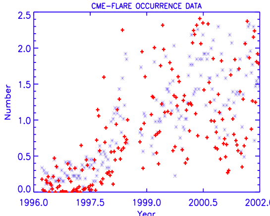
Figure 1: This graph illustrates the number of occurrences of CME and Halpa-flares normalized to their respective means are plotted with respect to year. The CME occurrences are represented with the stars in blue color and the flare occurrences are represented as plus signs with red color.

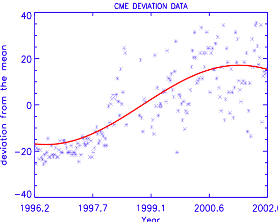
Figure 2: The figure illustrates the deviation from the mean of the CME occurrence with respect to year. The red continuous line superposed on the deviation data is fit of a sine curve of the form $y=Asin(\omega t+\phi)$, where $y$ is the deviation of the CME occurrences from the mean, $A=-17.03$ is amplitude, $\omega=2\pi/T$ (T= 9.3 yrs) is the frequency and $\phi(=1.22$ radians) is the phase.

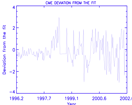
Figure 3: The figure represents the difference from the sine curve obtained from the least square fit and deviation from the mean of the CME occurrence plotted with respect to year. Notice a gap in the data during July 1998-Sept 1998 and Jan 1999.

In Fig 1, we present the occurrences of CME (in blue color) and flares (in red color) normalized to their respective means. After computing deviation from the mean of the CME occurrences, we fit a sine curve of the form $Asin(\omega t+\phi)$. Here A is the amplitude, $\omega\,(=2\pi/T,\,T\,is\,the\,period)$ is the frequency and $\phi$ is phase angle of the sine wave. Fitting a sine curve to the deviation data is a process of removing a long term trend of 11 years, although fitting of sine curve is not right as the profile of solar cycle is similar to profile of a solution obtained from the forced and damped harmonic oscillator (Hiremath 2006). In Fig 2, we present the deviation from the mean of the CME occurrences with a superposition of fitted sine curve (continuous line with a red color). We then compute the difference from the fitted sine curve and deviation from the mean data and the result is presented in Fig 3.

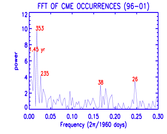
Figure 4: The figure illustrates the Scargle Fourier power spectrum of the CME occurrences with the gaps during July 1998-Sept 1998 and Jan 1999. The numbers in red color are periods whose powers are more than 3 $\sigma$ significance level. Except 1.45 yr period, rest of the detected periods are in days.

Owing to gaps in the data of the CME occurrences, we apply the Scargle (1989) method of Fourier analysis for the unevenly spaced data and whose Fourier transform is presented in Fig 4. We detect the periodicities 1.45 yr., 353 days, 235 days, 38 days and 26 days with the powers whose significance are greater than 3 $\sigma$ level. Though periods with significant powers appear to be almost similar to the periods detected in other solar activity indices, a large gap of 90 days and 30 days may act as sine waves and may induce spurious periods in the Fourier analysis. For example, spurious periods may be detected in the multiples (e.g. for the 90 day gaps, we may get 270 day and 360 day) of harmonics. In order to rule out such spurious periods, one way is to interpolate between the data gaps and make the data of equal intervals for applying the usual Fast Fourier transform (FFT). Since the duration of the data gap is very large, interpolation method may not fill accurately the data gaps. Another way to solve this problem is as follows. It is well established that solar x-ray flares are well associated with the coronal mass ejections (Harrison 1995). Assuming that such association may also exists (in the following analysis we find a very good correlation) between the H- alpha flare and the CME occurrence, we use H-alpha flare occurrence data in the following analysis for the correlative study. Then from the linear least square fit between the CME and H-alpha flare occurrences, we fill the data gaps for applying the usual FFT for the subsequent analysis.

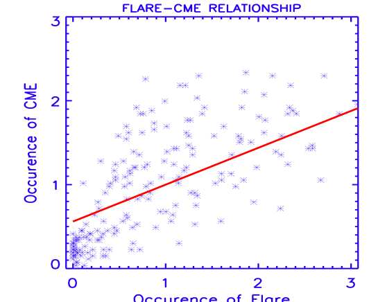
Figure 5: The figure represents a good correlation (65 %) between the CME and the flare occurrences normalized to their respective means. The superposed continuous straight line in red color is a linear least square fit for both the data set. The least square fit yields a straight line $CME=A+B(flare)$, where $A=0.56\pm 0.01$ and $B=0.44\pm 0.08$. From this relation and the known flare occurrences during the months of Jul 1998-Sept 1998 and Jan 1999, we fill the CME occurrence data during those gapped months.

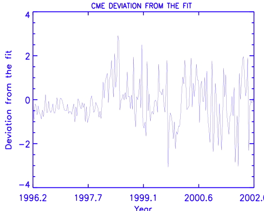
Figure 6: This figure is similar to that of the Fig 3 with a difference that the occurrence data is filled during the gapped months (July 1998-Sept 1998 and Jan 1999) of CME observations.

In Fig 5, we present the relation between the occurrence of CME and flare data normalized to their respective means. Notice a very good correlation ( 65 % ) of CME occurrences with the H-alpha flare occurrences. From the $z$ statistics (Fisher 1930), the probability of the correlation coefficient is found to be significant below less than 1 $\%$ indicating a very good correlation. Presently, we can not conclude whether production of CMEs lead to the production of the H-alpha flares and vice. verse. It appears that the occurrences of CME and H-alpha flare activities have one to one correspondence and may be symptom of the same physical phenomenon in different activities ( see also Zang et. al., 2001). The occurrences of CME and flare data are fitted with a straight line (red continuous line superposed on Fig 5) of the form CME = A + B (flare), where ’CME’ is the CME occurrences and ’flare’ is the H-alpha flare occurrences, A = $0.56\pm 0.01$ and B = $0.44\pm 0.08$. Using this law and known flare occurrences during the months of July 1998-Sept 1998 and Jan 1999, we fill the data gaps of the CME occurrences during those months. Totally we have 2120 day of observations and 212 data points for the 10 -day intervals. Then we fit a sine curve to the deviation from the mean of the filled CME occurrence data. The difference between deviation from the mean and the fit of the sine curve is presented in Fig 6. Except for the period of July 1998-Sept 1998 and Jan 1999, this plot is almost similar to the plot presented in the Figure 3.

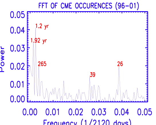
Figure 7: This figure illustrates the power spectrum obtained from the FFT analysis with equal intervals in time of the filled CME occurrence. The numbers in red colors are the periods detected with significance of their powers more than 3 $\sigma$ level. The periods 1.92 and 1.2 are in years and rest of the detected periods are in days.

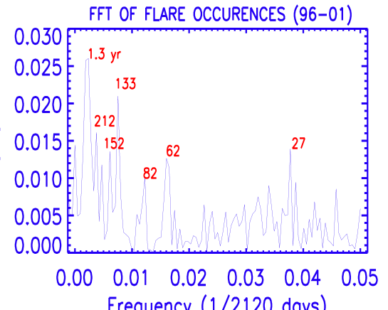
Figure 8: This figure illustrates the power spectrum of the flare occurrences from the FFT analysis with equal intervals in time. The numbers in red colors are the periods detected with significance of their powers more than 3 $\sigma$ level. The period 1.3 is in years and rest of the detected periods are in days.

In Fig 7, we present Fourier power spectrum of the CME occurrences for the equally spaced data of the resulting difference from the sine wave fit. From this analysis, we recovered all the periodicities as in the power spectrum of the gaped data with a much better peak at 1.2 yr. periodicity which is detected in almost all of the solar activity indices. It is surprising that the periodicity around 150 days, found in most of the activity indices, is absent in the CME occurrences even with the filled data. In fact we Fourier analyzed separately the difference data for the years March 1996-June 1998 and Feb 1999-Dec 2001 and, we could not detect the periodicity around 150 days. This absence of around 150 days periodicity is also consistent with the previous study (Lou et. al. 2003). In Fig 8, we present Fourier power spectrum of the flare data and we detect the periodicities 1.3yr. 212day, 152 day, 133 day, 82 day, 62 day and 27 day whose powers are greater than 3 $\sigma$ confidence level.

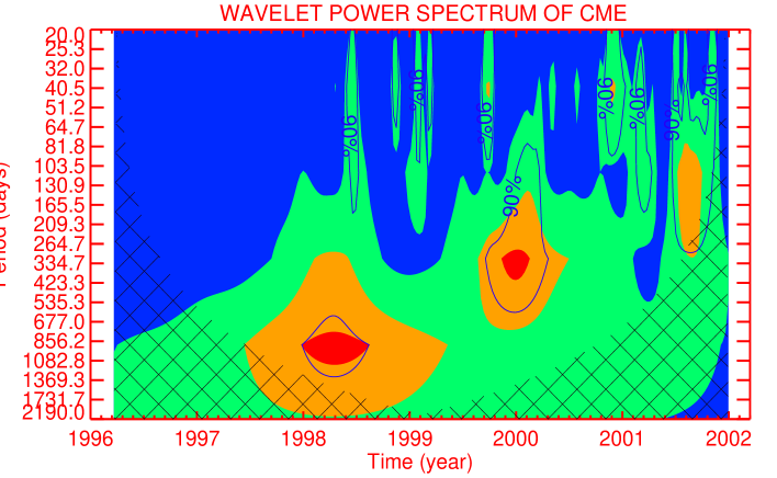
Figure 9: The figure represents the wavelet power spectrum of the CME occurrences with filled data set. The regions in the interior of the contours with a light blue color represents concentration of the power with a confidence level of $90\%$ significance and the power which is insignificant is present in the crossed hatched grey regions.

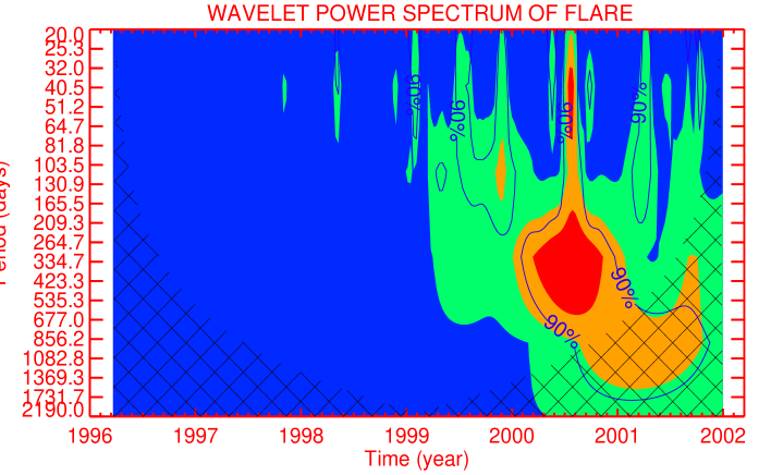
Figure 10: This illustration represents the wavelet power spectrum of the flare occurrences. The regions in the interior of the contours with a light blue color represents concentration of the power with a confidence level of $90\%$ significance and the power which is insignificant is present in the crossed hatched grey regions.

In order to know whether the detected periods of either CME or flare occurrences are continuous through out the observed period, we subject both the difference data set of filled CME and flare occurrences to the wavelet analysis. In Fig 9, we present power spectrum of the wavelet analysis of the filled CME occurrences and in Fig 10, we present the wavelet power spectrum of the occurrences of the flares. The decreasing order of wavelet power is represented as follows : the highest power in red, the next power in pink, the green and the blue having the least powers. The wavelet power in the gray hatched is not significant due to the fact that the data has been padded with zeros before applying the wavelet spectrum. It is crucial to be noted that all the periodicities detected from the Fourier analyses are also present in the wavelet power spectrum (concentrations of the wavelet power in the interior regions of light blue contours, which are significant at 90 % confidence levels). One disadvantage of the wavelet power spectrum is that we can not separate the periodic structures as in usual FFT method. It is to be noted that the activity of the CME and flare occurrences for the short periods, below one year, start simultaneously near the maximum of the solar activity. However, the activity of the long period H-alpha flare activity, especially 1.3 yr., begin around the maximum period has a phase lag of nearly six months compared to the long periods of CME activity. To be precise, the flare activity of long periods lags behind the CME activity of the long periods nearly by six months. Another interesting result to be noted is that all the dominant near 150 day and 1.3 year periodicities of the flare activity excite simultaneously around the middle of maximum year 2000. On the other hand, the CME activity of the long periods ( 1.2 and 1.9 year ) excite in different times.

3 Conclusions and Discussion

From the constraint of the CME data set from 1996-2001, presently it is not clear whether CME periodic activity of short and long periods behaved similarly in the previous solar cycles. Analyses of either future observed cycles of CME activity or analyses of proxy data such as flares, microwave bursts and auroras may give clear picture of the CME occurrence periodic activity. Over all conclusion from the present analysis is that the FFT and the wavelet analyses of the CME occurrences lead to discovery of the periodicities 1.92 yr., 1.2 yr., 265 day, 39 day and 26 day which are almost similar to the well known periodicities found in different solar activity indices. It is known fact (Olive, J.P, Chaloupy, M & Schweitzer 2002) that the station keeping maneuvers are limited to 4-6 months and SOHO orbit has 6-month period. In fact we have a peak (from the frequency range 0.035-0.052 in Fig 4 & from the frequency range 0.0083-0.0056 in Fig 7) around 4-6 months which is below the detection ( 3$\sigma$) level. From the wavelet analysis, it is found that the long period CME activity starts near the solar maximum. The comparative study of the wavelet power spectrums of the occurrences of the CME and the flare data suggests that the long period flare activity lags behind the long period CME activity nearly by six months.

As for the genesis of the long periodicities detected in the CME occurrence, some more years of occurrence data is required to give any meaningful physical interpretation. However, the 1.2 yr quasi-periodicity is almost similar to 1.3 yr quasi-periodicity that is discovered in many indices of solar cycle and activity phenomena. Recently Hiremath (2009b) has proposed new ideas on the physics of the solar cycle. It is proposed that sun is pervaded by a combined weak poioidal and strong toroidal magnetic field structure of primordial origin whose diffusion time scales are $\sim$ billion yrs. While explaining the near 11 yr sunspot (or 22 yr magnetic) cycle, physical inferences suggest that near 1.3 yr periodicity is due to long period Alfven wave perturbations to the ambient strong toroidal magnetic field structure near base of convection zone that travel to the surface near maximum of solar cycle and occur near the 20-25 deg latitude (or 70-75 deg colatitude) zone. Further details can be found from that study (see section 5.2.2 of Hiremath 2009b).

Acknowledgments

This paper is dedicated to my beloved parents who constantly encouraged my research carrier when they were alive. The CME catalog is generated and maintained by the center for Solar physics and Space Weather, The Catholic University of America in Cooperation with the Naval Research Laboratory and NASA. SOHO is a project of international cooperation between ESA and NASA. We used the wavelet software developed by C. Torrence and G. Compo and is available at the web site http://paos.colorado.edu/research/wavelets/.

4 References

Antia, H. M. & Basu, S., 2000, ApJ, 541, 442

Bai, T, 1987, ApJ, 318, L85

Ballester, J. L., & Baudin, F., 1998, Nature, 394, 552

Ballester, J. L., Oliver, R. & Carbonell, M., 2002, ApJ, 566, 505

Balthasar, H., 2007, A&A, 471, 281

Carbonell, M. & Ballester, J. L., 1990, A & A, 238, 377

Chowdhury, P., Manoranjan, K and Ray, P. C., 2009, MNRAS, 392, 1159

Delache, P. Laclare, F and Sadsaoud, H., 1985, Nature, 317, 416

Dimitropoulou, M., Moussas, X and Strintzi, D., 2008, MNRAS, 386, 2278

Droge, W. et. al., 1990, Astrophys. J, Supp, 73, 279

Fisher, R. A., 1930, in Statistical Methods for Research Workers, p. 74 & p. 168

Harrison, R. A., 1995, A& A, 304, 585

Hiremath, K. M., 1994, Ph. D Thesis, Study of Sun’s long period oscillations, Bangalore University, India

Hiremath, K. M., 2002, in Proc. IAU Coll 188, (ESA SP-505), p. 425

Hiremath, K. M., 2006, A&A, 452, 591

Hiremath, K. M., 2009a, accepted in Sun and Geosphere, also see the eprint: arXiv:0906.3110

Hiremath, K. M., 2009b, see the arXiv eprint

Howe, R., Cristensen-Dalsgaard, J., Hill, F., et. al., 2000, Science, 287, 2456

Ichimota, K., et. al., 1985, Nature, 316, 422

Javaraiah, J and Komm, R. W., 1999, Sol. Phys, 184, 41

Javaraiah, J., 2000, Ph. D. Thesis, Study of Sun’s rotation and solar activity, Bangalore University, India

Kane, R. P., Vats, H. O. and Sawant, H. S., 2001, Sol. Phys., 2011, 181

Kane, R. P., 2002, Sol. Phys., 205, 351

Kilic, H., 2009, Sol. Phys., 255, 155

Knaack, R.; Stenflo, J. O.; Berdyugina, S. V., 2005, A&A, 438, 1067

Krivova, N. A. & Solanki, S. K., 2002, A & A, 394, 701

Lara, A; Borgazzi, A; Mendes, Odim, Jr.; Rosa, R. R.; Domingues, M. O, 2008; Solar Physics, 248, 155

Lean, J. L & Brueckner, G. E., 1989, ApJ, 337, 568

Lean, J. L., 1990, ApJ, 363, 718

Lean, J. L, 1991, Rev. Geophys., 29, 4, 505

Leighton, R. B, 1960, in Proc. IAU Symp., 12, 321

Lou, Yu-Qing; Wang, Yu-Ming; Fan, Zuhui; Wang, Shui; Wang, Jing Xiu, 2003, MNRAS, 345, 809

Obridko, V. N and Shelting, B. D., 2007, Advan in Space Res, 40, 1006

Oliver, R., Carbonell, M. & Ballester, L., 1992, Sol. Phys., 137, 141

Olive, J.P, Chaloupy, M & Schweitzer, H., 2002, IAU coll 188, (ESA SP-505), p. 41

Pap, J., Tobiska, W. K. & Bouwer, S. D., 1990, Sol. Phys., 129, 165

Ribes, E., Merlin, Ph., Ribes, J.-C and Barthalot, R., 1989, An Geophys, 7, 321

Rieger, E. et. al., 1984, Nature, 312, 623

Scargle, J., 1989, ApJ, 343, 874

Singh, J. & Prabhu, T. P., 1985, Sol. Phys., 97, 203

Sturrock, P. A., Walther, G and Wheatland, M. S., 1997, ApJ, 491, 409

Vecchio, A.; Carbone, V., 2009, A&A, 502, 981

Verma, V. K.; Joshi, G. C.; Uddin, Wahab; Paliwal, D. C., 1991, A&AS, 90, 83

Wolff, C. L., 1983, ApJ, 264, 667

Zang, J., et. al., 2001, ApJ, 452, 2001