The Equation of State of Tracker Fields

Abstract

We derive the equation of state of tracker fields, which are typical examples of freezing quintessence (quintessence with the equation of state approaching toward $-1$), taking into account of the late-time departure from the tracker solution due to the nonzero density parameter of dark energy $\Omega_{\phi}$. We calculate the equation of state as a function of $\Omega_{\phi}$ for constant $\Gamma=VV^{\prime\prime}/(V^{\prime})^{2}$ (during matter era) models. The derived equation of state contains a single parameter, $w_{(0)}$, which parametrizes the equation of state during the matter-dominated epoch. We derive observational constraints on $w_{(0)}$ and find that observational data are consistent with the cosmological constant: $-1.11<w_{(0)}<-0.96(1\sigma)$.

I Introduction

There is strong evidence that the Universe is dominated by dark energy. Moreover, the cosmological constant fits the current observational data quite well. However, how much is a dark energy model close to the cosmological constant? In order to quantify such ”distance from the cosmological constant” in the dark energy theory space, we need to introduce a parametrization of the equation of state, $w(a)$, which parametrizes the deviation from the cosmological constant, $w=-1$.

In our former study ds ; chiba ; cds , we derived the equation of state for certain scalar field dark energy (quintessence quint / k-essence kess ) models under the assumption such that the scalar field slow rolls ($w\simeq-1$) during the matter dominated era. Such quintessence exhibits thawing behavior cl : the scalar field freezes during the matter era and gradually moves after the dark energy dominated era so that the equation of state deviates from $w\simeq-1$. We find our parametrization applies both to thawing quintessence models and to a subset of thawing k-essence models with $w\simeq-1$.

However, there are quintessence models which evolve the opposite: freezing models cl with $w$ approaching toward $w=-1$ so that the scalar field gradually freezes its motion. In this paper, we derive the equation of state for a class of freezing quintessence models called tracker fields swz whose equation state is nearly constant during the matter-dominated era. For freezing models, the equation of state deviates from $-1$ during the matter era so that the slow-roll approximation is not a good approximation. Instead, we solve the equation of motion by expanding around the tracker solution (the solution to which the tracker field converges from various initial conditions). The equation of state up to first order in the density parameter of dark energy $\Omega_{\phi}$ was derived by ws for an inverse power-law potential power1 . We extend the solution to higher orders in $\Omega_{\phi}$ and present a useful approximation to the equation of state for tracker fields. Hence we now have a physically motivated parametrization of $w$ both for thawing quintessence and for (a class of) freezing quintessence.

Apart from these motivations, it is also useful to derive $w(a)$ for more practical purposes because we do not need to solve the equation of motion directly for each potential. The idea has similarity, in spirit, with the slow-roll conditions: the existence of inflationary solutions reduces to simple conditions without having to solve the equation of motion directly.

The paper is organized as follows: In Sec. 2, by perturbing the tracker equation, we derive the equation of state for tracker fields to all orders in $\Omega_{\phi}$. In Sec. 3, we derive the observational constraints on the parameter of the equation of state from Type Ia supernovae (SNIa) data and baryon acoustic oscillations (BAO). Sec. 4 is devoted to summary.

II Solving Tracker Equation

We consider a flat universe consisting of background matter and scalar field dark energy $\phi$. The equation of motion of $\phi$ is

$$\ddot{\phi}+3H\dot{\phi}+V^{\prime}(\phi)=0,$$ (1)

where $V^{\prime}=\partial V/\partial\phi$. The equation of state $w$ is given by

$$w=\frac{\dot{\phi}^{2}/2-V}{\dot{\phi}^{2}/2+V}.$$ (2)

The equation of motion Eq.(1) can be rewritten by using $w$ swz :

$$\mp\frac{V^{\prime}}{V}=\sqrt{\frac{3\kappa^{2}(1+w)}{\Omega_{\phi}(a)}}\left(1+\frac{\dot{x}}{6}\right),$$ (3)

where the minus sign corresponds to $\dot{\phi}>0(V^{\prime}<0)$ and the plus sign to the opposite, $\kappa^{2}=8\pi G$, $\Omega_{\phi}(a)$ is the density parameter of dark energy, $x=(1+w)/(1-w)$ and $\dot{x}\equiv{d\ln x}/{d\ln a}$. Tracker fields have nearly constant $w$ initially and eventually evolve toward $w=-1$.

II.1 Tracker Solution

Tracker fields have attractor-like solutions in the sense that a very wide range of initial conditions rapidly converge to a common cosmic evolutionary track: the tracker solution swz . Taking the derivative of Eq.(3) with respect to $\phi$, we obtain the so-called tracker equation rubano ; scherrer05 ; ktrac

$$\Gamma-1\equiv\frac{VV^{\prime\prime}}{V^{\prime 2}}-1=\frac{w_{B}-w}{2(1+w)}-\frac{(1+w_{B}-2w)\dot{x}}{2(1+w)(6+\dot{x})}+\frac{3(w-w_{B})\Omega_{\phi}(a)}{(1+w)(6+\dot{x})}-\frac{2\ddot{x}}{(1+w)(6+\dot{x})^{2}},$$ (4)

where $w_{B}$ is the equation of state of background matter and $\ddot{x}\equiv d^{2}\ln x/d\ln a^{2}$. Equation (4) differs from the tracker equation in swz where the term involving $\Omega_{\phi}$ is neglected which is essential in deriving the perturbation solution of $w$.

Henceforth we consider the epoch after the matter-dominated era, so that we set $w_{B}=0$. Since during the matter-dominated epoch $\Omega_{\phi}$ is negligible and $w$ becomes an almost constant for tracker fields, $w$ in that epoch is written in terms of $\Gamma$ as swz ; ws

$$w_{(0)}=-\frac{2(\Gamma_{(0)}-1)}{1+2(\Gamma_{(0)}-1)},$$ (5)

where the zero subscript in parentheses denotes the zeroth-order solution, neglecting the contribution of dark energy to the expansion rate.

II.2 Perturbing the Tracker Evolution

In order to include the effect of finite $\Omega_{\phi}$, we treat it as a perturbation to the zeroth-order solution and then extrapolate the result to the situation where $\Omega_{\phi}$ is not so small when comparing the solution with the numerical solution.

We define the perturbation to the zeroth-order solution $w_{(0)}$ to be $\delta w$, where $\delta w\sim\delta\phi/\phi\sim{\cal O}(\Omega_{\phi})$ from Eq. (3) ws . Keeping all terms of order $\Omega_{\phi}$ in Eq. (4), we obtain

$$a^{2}\frac{d^{2}\delta w}{da^{2}}+\frac{5-6w_{(0)}}{2}a\frac{d\delta w}{da}+\frac{9}{2}(1-w_{(0)})\delta w-\frac{9}{2}w_{(0)}(1-w_{(0)}^{2})\Omega_{\phi}(a)+9(1-w_{(0)}^{2})(1+w_{(0)})d\Gamma=0.$$ (6)

We find that the analysis can be made simpler if $\Gamma={\rm constant}$ so that the last term in Eq.(6) is vanishing. This is the case for inverse power-law potentials and for exponential potentials. In fact, for $V=M^{4}(M/\phi)^{\alpha}$, $\Gamma=(1+\alpha)/\alpha$, and also for $V=M^{4}e^{\lambda\kappa\phi}$, $\Gamma=1$. We limit ourselves to the case when this holds so that we can solve Eq. (6) without using $\delta\phi$. Note that this condition does not hold for a constant $w$ model lopez and for an exponential of inverse power-law model: $V=M^{4}\exp(1/\kappa\phi)$ swz .

By approximating $\Omega_{\phi}$ by the zeroth-order solution and expanding it in terms of the scale factor (or $\rho_{\phi_{(0)}}/\rho_{B}$) as

$$\Omega_{\phi}(a) = \frac{\Omega_{\phi 0}a^{-3w_{(0)}}}{\Omega_{\phi 0}a^{-3w_{(0)}}+(1-\Omega_{\phi 0})}$$ (7)

$$= \sum_{n=1}^{\infty}(-1)^{n-1}\left(\frac{\Omega_{\phi 0}}{1-\Omega_{\phi 0}}\right)^{n}a^{-3nw_{(0)}}$$

we find, to all orders in $\rho_{\phi_{(0)}}/\rho_{B}$ or in $\Omega_{\phi}$,

$$w(a)=w_{(0)}+\delta w = w_{(0)}+\frac{(1-w_{(0)}^{2})w_{(0)}}{1-2w_{(0)}+4w_{(0)}^{2}}\frac{\Omega_{\phi 0}}{1-\Omega_{\phi 0}}a^{-3w_{(0)}}-\frac{(1-w_{(0)}^{2})w_{(0)}}{1-3w_{(0)}+12w_{(0)}^{2}}\left(\frac{\Omega_{\phi 0}}{1-\Omega_{\phi 0}}\right)^{2}a^{-6w_{(0)}}+\dots$$

$$= w_{(0)}+\sum_{n=1}^{\infty}\frac{(-1)^{n-1}w_{(0)}(1-w_{(0)}^{2})}{2n(n+1)w_{(0)}^{2}-(n+1)w_{(0)}+1}\left(\frac{\Omega_{\phi 0}}{1-\Omega_{\phi 0}}\right)^{n}a^{-3nw_{(0)}},$$

$$= w_{(0)}+\sum_{n=1}^{\infty}\frac{(-1)^{n-1}w_{(0)}(1-w_{(0)}^{2})}{2n(n+1)w_{(0)}^{2}-(n+1)w_{(0)}+1}\left(\frac{\Omega_{\phi}(a)}{1-\Omega_{\phi}(a)}\right)^{n},$$

$$= w_{(0)}+\frac{(1-w_{(0)}^{2})w_{(0)}}{1-2w_{(0)}+4w_{(0)}^{2}}\Omega_{\phi}(a)+\frac{(1-w_{(0)}^{2})w_{(0)}^{2}(8w_{(0)}-1)}{(1-2w_{(0)}+4w_{(0)}^{2})(1-3w_{(0)}+12w_{(0)}^{2})}\Omega_{\phi}(a)^{2}$$

$$+\frac{2(1-w_{(0)}^{2})w_{(0)}^{3}(4w_{(0)}-1)(18w_{(0)}+1)}{(1-2w_{(0)}+4w_{(0)}^{2})(1-3w_{(0)}+12w_{(0)}^{2})(1-4w_{(0)}+24w_{(0)}^{2})}\Omega_{\phi}(a)^{3}+\dots$$

Eq. (II.2) is our main result. In the last equation, we have also expanded in terms of $\Omega_{\phi}(a)$ using $(\Omega_{\phi}(a)/(1-\Omega_{\phi}(a)))^{n}=\Omega_{\phi}(a)^{n}(\sum_{m=0}^{\infty}\Omega_{\phi}(a)^{m})^{n}$. Up to the second order in $\Omega_{\phi}$, the solution becomes

$$w_{2}(a)=w_{(0)}+\frac{(1-w_{(0)}^{2})w_{(0)}}{1-2w_{(0)}+4w_{(0)}^{2}}\Omega_{\phi}(a)+\frac{(1-w_{(0)}^{2})w_{(0)}^{2}(8w_{(0)}-1)}{(1-2w_{(0)}+4w_{(0)}^{2})(1-3w_{(0)}+12w_{(0)}^{2})}\Omega_{\phi}(a)^{2}.$$ (9)

Note that $w(a)=-1$ if $w_{(0)}=-1$ and hence the cosmological constant is contained in our $w(a)$. This $w(a)$ (or $w_{2}(a)$) agrees with the solution found in ws (their Eq. (33)) up to the first order in $\Omega_{\phi}$:

$$w_{ws}(a)=w_{(0)}+\frac{(1-w_{(0)}^{2})w_{(0)}}{1-2w_{(0)}+4w_{(0)}^{2}}\Omega_{\phi}(a).$$ (10)

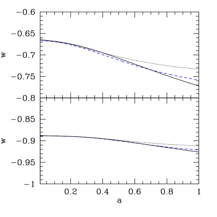
Figure 1: Evolution of $w(a)$ for inverse power-law potentials: $V=M^{4}(M/\phi)^{\alpha}$. The upper plot corresponds to the $\alpha=1$ case and the lower one corresponds to the $\alpha=1/4$ case. The solid (black) lines denote the numerical result, the dashed (blue) lines denote the second order solution $w_{2}(a)$ given by Eq. (9), and the dotted lines denote the first order solution $w_{ws}(a)$ Eq. (10).

We find the second order solution $w_{2}(a)$ Eq. (9) already agrees with the numerical solutions fairly well as shown in Fig. 1. For $\alpha\leq 1$ (or $w_{(0)}\leq-2/3$), the fractional error of the equation of state between the numerical solutions and $w_{2}(a)$, Eq. (9), is less than 1.8%, while the error can be as large as 5% for $w_{ws}$.

III Observational Constraints on $w_{(0)}$

We present the observational constraints on the equation of state parameters $w_{(0)}$. We use the second order equation of state $w_{2}(a)$ Eq. (9) for simplicity.

As observational data we consider the recent compilation of 397 SNIa, called the Constitution Set with the light curve fitter SALT, by Hicken et al. hicken and the measurements of BAO from the recent SDSS data baonew which is now consistent with both earlier SDSS data bao and 2dF data percival . Uncertainties in the distance modulus of a supernova include uncertainties in light curve fitting parameters (the maximum magnitude, stretch parameter, color correction parameter) and due to the peculiar velocity (400 ${\rm kms^{-1}}$) as given in hicken .

BAO measurements from the SDSS data provide a constraint on the distance parameter $A$ defined by

$$A(z)=(\Omega_{m}H_{0}^{2})^{1/2}\left(\frac{1}{H(z)z^{2}}\right)^{1/3}\left(\int^{z}_{0}\frac{dz^{\prime}}{H(z^{\prime})}\right)^{2/3}$$ (11)

to be $A(z=0.35)=0.493\pm 0.017$ baonew .

The $\chi^{2}$ curve normalized by its minimum, $\Delta\chi^{2}=\chi^{2}-\chi^{2}_{min}$, calculated from SNIa and BAO is shown in Fig. 2. We marginalize over $\Omega_{m}$ to calculate the curve. The allowed range of $w_{(0)}$ is narrow: $-1.11<w_{(0)}<-0.96(1\sigma)$, $-1.19<w_{(0)}<-0.90(2\sigma)$, $-1.28<w_{(0)}<-0.84(3\sigma)$.

Figure 2: $\Delta\chi^{2}$ as a function of $w_{(0)}$.

IV Summary

We have derived the equation of state for a class of freezing quintessence models called tracker fields whose equation state is nearly constant during the matter-dominated era. By solving the tracker equation perturbatively, we could derive a useful approximated solution to the equation of state for tracker fields (Eq. (II.2)). The solutions agree with the numerical solutions quite accurately.

Our solution is also useful for pragmatic purposes in that one only have to use our equation of state without solving the scalar field of motion numerically for any power index $\alpha$.

Applying the solution of $w(a)$ truncated to the second order in $\Omega_{\phi}$, $w_{2}(a)$, to SNIa data and BAO, we find that the parameter $w_{(0)}$, which parameterizes the equation of state during the matter-dominated era, is constrained to lie near $-1$ and hence the cosmological constant limit of these models is consistent with the current data.

Combining with our previous results on thawing models ds ; chiba ; cds , we now have three parameters ($w_{0},K,w_{(0)}$) for the equation of state both for thawing models and for (a class of) freezing models:

$$1+w(a)=\left\{\begin{array}[]{lr}(1+w_{0})a^{3(K-1)}\left(\frac{(K-F(a))(F(a)+1)^{K}+(K+F(a))(F(a)-1)^{K}}{(K-\Omega_{\phi 0}^{-1/2})(\Omega_{\phi 0}^{-1/2}+1)^{K}+(K+\Omega_{\phi 0}^{-1/2})(\Omega_{\phi 0}^{-1/2}-1)^{K}}\right)^{2}&\mbox{(thawing quintessence)},\\ 1+w_{(0)}+\sum_{n=1}^{\infty}\frac{(-1)^{n-1}w_{(0)}(1-w_{(0)}^{2})}{2n(n+1)w_{(0)}^{2}-(n+1)w_{(0)}+1}\left(\frac{\Omega_{\phi}(a)}{1-\Omega_{\phi}(a)}\right)^{n}&\mbox{(freezing quintessence)},\end{array}\right.$$ (14)

where $F(a)=\sqrt{1+(\Omega_{\phi 0}^{-1}-1)a^{-3}}$. In this dark energy theory space, dark energy is close to the cosmological constant, which corresponds to $w_{0}=-1$ irrespective of $K$ and $w_{(0)}=-1$, to the extent such that: $-1.14<w_{0}<-0.92,-1.11<w_{(0)}<-0.96$ and no constraint on $K$.

References

(1)
S. Dutta and R. J. Scherrer,
Phys. Rev. D 78, 123525 (2008)
[arXiv:0809.4441 [astro-ph]].
(2)
T. Chiba,
Phys. Rev. D 79, 083517 (2009)
[Erratum-ibid. D 80, 109902 (2009)]
[arXiv:0902.4037 [astro-ph.CO]].
(3)
T. Chiba, S. Dutta and R. J. Scherrer,
Phys. Rev. D 80, 043517 (2009)
[arXiv:0906.0628 [astro-ph.CO]].
(4)
R. R. Caldwell, R. Dave and P. J. Steinhardt,
Phys. Rev. Lett. 80, 1582 (1998).
(5)
T. Chiba, T. Okabe and M. Yamaguchi,
Phys. Rev. D 62, 023511 (2000)
[arXiv:astro-ph/9912463];
C. Armendariz-Picon, V. F. Mukhanov and P. J. Steinhardt,
Phys. Rev. Lett. 85, 4438 (2000)
[arXiv:astro-ph/0004134].
(6)
R. R. Caldwell and E. V. Linder,
Phys. Rev. Lett. 95, 141301 (2005)
[arXiv:astro-ph/0505494].
(7)
P. J. Steinhardt, L. M. Wang and I. Zlatev,
Phys. Rev. D 59, 123504 (1999).
(8)
C. R. Watson and R. J. Scherrer,
Phys. Rev. D 68, 123524 (2003)
[arXiv:astro-ph/0306364].
(9)
B. Ratra and P. J. E. Peebles,
Phys. Rev. D 37, 3406 (1988).
(10)
C. Rubano, P. Scudellaro, E. Piedipalumbo, S. Capozziello and M. Capone,
Phys. Rev. D 69, 103510 (2004)
[arXiv:astro-ph/0311537].
(11)
R. J. Scherrer,
Phys. Rev. D 73, 043502 (2006)
[arXiv:astro-ph/0509890].
(12)
T. Chiba,
Phys. Rev. D 66, 063514 (2002)
[arXiv:astro-ph/0206298].
(13)
L. A. Urena-Lopez and T. Matos,
Phys. Rev. D 62, 081302 (2000)
[arXiv:astro-ph/0003364].
(14)
M. Hicken et al.,
Astrophys. J. 700, 1097 (2009)
[arXiv:0901.4804 [astro-ph.CO]].
(15)
B. A. Reid et al.,
arXiv:0907.1659 [astro-ph.CO];
W. J. Percival et al.,
arXiv:0907.1660 [astro-ph.CO].
(16)
D. J. Eisenstein et al. [SDSS Collaboration],
Astrophys. J. 633, 560 (2005)
[arXiv:astro-ph/0501171].
(17)
W. J. Percival, S. Cole, D. J. Eisenstein, R. C. Nichol, J. A. Peacock, A. C. Pope and A. S. Szalay,
Mon. Not. Roy. Astron. Soc. 381, 1053 (2007)
[arXiv:0705.3323 [astro-ph]].