Secular evolution of a satellite by tidal effect. Application to Triton.

Abstract

Some of the satellites in the Solar System, including the Moon, appear to have been captured from heliocentric orbits at some point in their past, and then have evolved to the present configurations. The exact process of how this trapping occurred is unknown, but the dissociation of a planetesimal binary in the gravitational field of the planet, gas drag, or a massive collision seem to be the best candidates. However, all these mechanisms leave the satellites in elliptical orbits that need to be damped to the present almost circular ones. Here we give a complete description of the secular tidal evolution of a satellite just after entering a bounding state with the planet. In particular, we take into account the spin evolution of the satellite, which has often been assumed synchronous in previous studies. We apply our model to Triton and successfully explain some geophysical properties of this satellite, as well as the main dynamical features observed for the Neptunian system.

1. Introduction

Both the Earth’s Moon and Pluto’s moon, Charon, have an important fraction of the mass of their systems, and therefore they could be classified as double-planets rather than as satellites. The proto-planetary disk is unlikely to produce such systems, and their origin seems to be due to a catastrophic impact of the initial planet with a body of comparable dimensions (e.g. Canup and Asphaug, 2001; Canup, 2005). On the other hand, Neptune’s moon, Triton, and the Martian moon, Phobos, are spiraling down into the planet, clearly indicating that the present orbits are not primordial, and may have undergone a long evolving process from a previous capture (e.g. Mignard, 1981; Goldreich et al., 1989).

The present orbits of all these satellites are almost circular, and their spins appear to be synchronous with the orbital mean motion, as well as being locked in Cassini states (e.g. Colombo, 1966; Peale, 1969). This also applies to the Galilean satellites of Jupiter, which are likely to have originated from Jupiter’s accretion disk and additionally show orbital mean motion resonances (e.g. Yoder, 1979). All these features seem to be due to tidal evolution, which arises from differential and inelastic deformation of the planet by a perturbing body.

Previous long-term studies on the orbital evolution of satellites have assumed that their rotation is synchronously locked, and therefore limits the tidal evolution to the orbits (e.g. McCord, 1966). However, these two kinds of evolution cannot be dissociated because the total angular momentum must be conserved. Additionally, it has been assumed that the spin axis is locked in a Cassini state with very low obliquity. Although these assumptions are correct for the presently known situations, they were not necessarily true throughout the evolution.

The aim of this Letter is to model the orbital evolution of a satellite from its origin or capture until the preset day, including spin evolution for both planet and satellite, and also to make predictions regarding its future evolution. We provide a simple averaged model adapted for fast computational simulations, as required for long-term studies. In the last section we apply this model to the Triton-Neptune system.

2. The model

We consider a hierarchical system composed of a star, a planet and a satellite, with masses $M\gg m_{0}\gg m_{1}$, respectively. Both planet and satellite are considered oblate ellipsoids with gravity field coefficients given by $J_{2_{0}}$ and $J_{2_{1}}$, rotating about the axis of maximal inertia along the directions $\mathbf{\hat{s}}_{0}$ and $\mathbf{\hat{s}}_{1}$, with rotation rates $\omega_{0}$ and $\omega_{1}$, respectively. The potential energy $U$ of the system is then given by (e.g. Smart, 1953):

$$U = -G\frac{Mm_{0}}{r_{0}}\left(1-\sum_{i=0,1}J_{2_{i}}\frac{m_{i}}{m_{0}}\left(\frac{R_{i}}{r_{0}}\right)^{2}\!\!P_{2}(\mathbf{\hat{r}}_{0}\cdot\mathbf{\hat{s}}_{i})\right)$$ (3)

$$-G\frac{m_{0}m_{1}}{r_{1}}\left(1-\sum_{i=0,1}J_{2_{i}}\left(\frac{R_{i}}{r_{1}}\right)^{2}\!\!P_{2}(\mathbf{\hat{r}}_{1}\cdot\mathbf{\hat{s}}_{i})\right)$$

$$-G\frac{Mm_{1}}{r_{0}}\left(\frac{r_{1}}{r_{0}}\right)^{2}\!\!P_{2}(\mathbf{\hat{r}}_{0}\cdot\mathbf{\hat{r}}_{1})\ ,$$

where terms in $(R_{i}/r_{j})^{3}$ have been neglected ($i,j=0,1$). $G$ is the gravitational constant, $R_{i}$ the radius of the planet or the satellite, $\mathbf{r}_{i}$ the distance between the planet and the star or the satellite, and $P_{2}(x)=(3x^{2}-1)/2$ the Legendre polynomial of degree two.

Neglecting tidal interactions with the star, the tidal potential is written (e.g. Kaula, 1964):

$$U_{T}=-G\frac{m_{0}m_{1}}{r_{1}^{3}}\sum_{i=0,1}k_{2_{i}}\frac{R_{i}^{5}}{r_{i}^{\prime 3}}P_{2}(\mathbf{\hat{r}}_{1}\cdot\mathbf{\hat{r}}_{i}^{\prime})\ ,$$ (4)

where $k_{2_{i}}$ is the potential Love number for the planet or the satellite, and $\mathbf{r}_{i}^{\prime}$ the position of the interacting body at a time delayed of $\Delta t_{i}$. For simplicity, we will adopt a model with constant $\Delta t_{i}$, which can be made linear (e.g. Mignard, 1979; Hut, 1981; Néron de Surgy and Laskar, 1997):

$$\mathbf{r}_{i}^{\prime}\simeq\mathbf{r}_{1}+\Delta t_{i}\left(\omega_{i}\mathbf{s}_{i}\times\mathbf{r}_{1}-\mathbf{\dot{r}}_{1}\right)\ .$$ (5)

The complete evolution of the system can be tracked by the evolution of the rotational angular momentums, $\mathbf{H}_{i}\simeq C_{i}\omega_{i}\mathbf{\hat{s}}_{i}$, the orbital angular momentums, $\mathbf{L}_{i}\simeq m_{i}n_{i}a_{i}^{2}(1-e_{i}^{2})^{1/2}\mathbf{\hat{k}}_{i}$, and the orbital energy $E_{1}\simeq-Gm_{0}m_{1}/(2a_{1})$. $n_{i}$ is the mean motion, $a_{i}$ the semi-major axis, $e_{i}$ the eccentricity, and $C_{i}$ the principal moment of inertia. The contributions to the orbits are easily computed from the above potentials as

$$\mathbf{\dot{L}}_{0}=-\mathbf{r}_{0}\times\mathbf{\nabla}_{\!\mathbf{r}_{0}}U;\quad\mathbf{\dot{L}}_{1}=-\mathbf{r}_{1}\times\mathbf{\nabla}_{\!\mathbf{r}_{1}}U;\quad\dot{E}_{1}=-\mathbf{\dot{r}}_{1}\cdot\mathbf{\nabla}_{\!\mathbf{r}_{1}}U\ .$$ (6)

Since the total angular momentum is conserved, the contributions to the spin of the planet and satellite can easily be computed from the orbital contributions:

$$\mathbf{\dot{H}}_{0}+\mathbf{\dot{H}}_{1}+\mathbf{\dot{L}}_{0}+\mathbf{\dot{L}}_{1}=0\ .$$ (7)

Because tidal effects act in long-term time-scales, we further average the equations of motion over fast angles, namely the true anomaly and the longitude of the periapse. The resulting equations for the conservative motion are (e.g. Boué and Laskar, 2006):

$$\mathbf{\dot{L}}_{1}=-\gamma\cos I\,\mathbf{\hat{k}}_{0}\times\mathbf{\hat{k}}_{1}-\sum_{i}\beta_{i}\cos\theta_{i}\,\mathbf{\hat{s}}_{i}\times\mathbf{\hat{k}}_{1}\ ,$$ (8)

$$\mathbf{\dot{H}}_{i}=-\alpha_{i}\cos\varepsilon_{i}\,\mathbf{\hat{k}}_{0}\times\mathbf{\hat{s}}_{i}-\beta_{i}\cos\theta_{i}\,\mathbf{\hat{k}}_{1}\times\mathbf{\hat{s}}_{i}\ ,$$ (9)

where

$$\alpha_{i}=\frac{3GMm_{i}J_{2_{i}}R_{i}^{2}}{2a_{0}^{3}(1-e_{0}^{2})^{3/2}}\ ,$$ (10)

$$\beta_{i}=\frac{3Gm_{0}m_{1}J_{2_{i}}R_{i}^{2}}{2a_{1}^{3}(1-e_{1}^{2})^{3/2}}\ ,$$ (11)

$$\gamma=\frac{3GMm_{1}a_{1}^{2}(2+3e_{1}^{2})}{8a_{0}^{3}(1-e_{0}^{2})^{3/2}}\ ,$$ (12)

and

$$\cos\varepsilon_{i}=\mathbf{\hat{s}}_{i}\cdot\mathbf{\hat{k}}_{0}\ ,\quad\cos\theta_{i}=\mathbf{\hat{s}}_{i}\cdot\mathbf{\hat{k}}_{1}\ ,\quad\cos I=\mathbf{\hat{k}}_{0}\cdot\mathbf{\hat{k}}_{1}\ ,$$ (13)

are the direction cosines of the spins and orbits: $\varepsilon_{i}$ is the obliquity to the orbital plane of the planet, $\theta_{i}$ the obliquity to the orbital plane of the satellite, and $I$ the inclination between orbital planes.

For the dissipative tidal effects, we can obtain the equations of motion directly from equation (6), using $U_{T}$ instead of $U$, that is, $\mathbf{\dot{L}}_{0}=0$,

$$\mathbf{\dot{H}}_{i}=-K_{i}\,n_{1}\left(f_{1}(e_{1}){{\displaystyle\mathbf{\hat{s}}_{i}+\cos\theta_{i}\,\mathbf{\hat{k}}_{1}}\over{\displaystyle 2}}{{\displaystyle\omega_{i}}\over{\displaystyle n_{1}}}-f_{2}(e_{1})\mathbf{\hat{k}}_{1}\right)\ ,$$ (14)

$$\dot{E}_{1}=\sum_{i\neq j}K_{i}\,n_{1}^{2}\left(f_{2}(e_{1})\cos\theta_{i}{{\displaystyle\omega_{i}}\over{\displaystyle n_{1}}}-f_{3}(e_{1})\right)\ ,$$ (15)

where ($i,j=0,1$),

$$K_{i}=\Delta t_{i}(3k_{2_{i}}Gm_{j}^{2}R_{i}^{5})/a_{1}^{6}\ ,$$ (16)

and $f_{1}(e)=(1+3e^{2}+3e^{4}/8)/(1-e^{2})^{9/2}\ ,$ $f_{2}(e)=(1+15e^{2}/2+45e^{4}/8+5e^{6}/16)/(1-e^{2})^{6}\ ,$ $f_{3}(e)=(1+31e^{2}/2+255e^{4}/8+185e^{6}/16+25e^{8}/64)/(1-e^{2})^{15/2}\ .$

3. Secular evolution

In the previous section we presented the equations that rule the tidal evolution of a satellite in terms of angular momenta and orbital energy. However, the spin and orbital quantities are better represented by the rotation angles and elliptical elements. The direction cosines (Eq.13) are obtained from the angular momenta vectors, since $\mathbf{\hat{s}}_{i}=\mathbf{H}_{i}/||\mathbf{H}_{i}||$ and $\mathbf{\hat{k}}_{i}=\mathbf{L}_{i}/||\mathbf{L}_{i}||$, as well as the rotation rate $\omega_{i}=\mathbf{H}_{i}\cdot\mathbf{\hat{s}}_{i}/C_{i}$. The semi-major axis and the eccentricity can be obtained from $E_{1}$ and $||\mathbf{L}_{1}||$, respectively.

The variation in the satellite’s rotation rate can be computed from equation (14) as $\dot{\omega}_{i}=\mathbf{\dot{H}}_{i}\cdot\mathbf{\hat{s}}_{i}/C_{i}$, giving (Correia and Laskar, 2009):

$$\dot{\omega}_{1}=-\frac{K_{1}\,n_{1}}{C_{1}}\left(f_{1}(e_{1}){{\displaystyle 1+\cos^{2}\theta_{1}}\over{\displaystyle 2}}{{\displaystyle\omega_{1}}\over{\displaystyle n_{1}}}-f_{2}(e_{1})\cos\theta_{1}\right)\ .$$ (17)

For a given obliquity and eccentricity, the equilibrium rotation rate, obtained when $\dot{\omega}_{1}=0$, is attained for:

$$\frac{\omega_{1}}{n_{1}}=\frac{f_{2}(e_{1})}{f_{1}(e_{1})}\,\frac{2\cos\theta_{1}}{1+\cos^{2}\theta_{1}}\ ,$$ (18)

The obliquity variations can be obtained from equation (13):

$$\frac{d\cos\theta_{i}}{dt}=\frac{\dot{\mathbf{H}}_{i}\cdot(\mathbf{\hat{k}}_{1}-\cos\theta_{i}\mathbf{\hat{s}}_{i})}{||\mathbf{H}_{i}||}+\frac{\dot{\mathbf{L}}_{1}\cdot(\mathbf{\hat{s}}_{i}-\cos\theta_{i}\mathbf{\hat{k}}_{1})}{||\mathbf{L}_{1}||}\ .$$ (19)

For the conservative motion (Eqs. 8, 9), stable configurations for the spin can be found whenever the vectors ($\mathbf{\hat{s}}_{1}$, $\mathbf{\hat{k}}_{1}$, $\mathbf{\hat{k}}_{0}$) or ($\mathbf{\hat{s}}_{1}$, $\mathbf{\hat{k}}_{1}$, $\mathbf{\hat{s}}_{0}$) are coplanar and precess at the same rate $g$ (e.g. Colombo, 1966; Peale, 1969). The first situation occurs if $\gamma\gg\beta_{0}$ (outer satellite) and the second situation when $\gamma\ll\beta_{0}$ (inner satellite). The equilibrium obliquities can be found from a single relationship (e.g. Ward and Hamilton, 2004):

$$\lambda_{1}\cos\theta_{1}\sin\theta_{1}+\sin(\theta_{1}-I_{0})=0\ ,$$ (20)

where $\lambda_{1}=\beta_{1}/(C_{1}\omega_{1}g)$ is a dimensionless parameter and $I_{0}$ is the inclination of the orbit of the satellite with respect to the Laplacian plane ($I_{0}\simeq I$ and $g\simeq\gamma\cos I/||\mathbf{L}_{1}||$ for an outer satellite, and $I_{0}\simeq\theta_{0}$ and $g\simeq\beta_{0}\cos\theta_{0}/||\mathbf{L}_{1}||$ for an inner satellite) (e.g. Laplace, 1799; Mignard, 1981; Tremaine et al., 2009). The above equation has two or four real roots for $\theta_{1}$, which are known by $Cassini$ $states$. In general, for satellites we have $I_{0}\sim 0$, and these solutions are approximately given by:

$$\tan^{-1}\left(\frac{\sin I_{0}}{\cos I_{0}\pm\lambda_{1}}\right)\ ,\quad\pm\cos^{-1}\left(-\frac{\cos I_{0}}{\lambda_{1}}\right)\ .$$ (21)

For a generic value of $I_{0}$, when $\lambda_{1}\ll 1$, which is often the case of an outer satellite, the first expression gives the only two real roots of equation (20), one for $\theta_{1}\simeq I_{0}$ and another for $\theta_{1}\simeq\pi-I_{0}$. On the other hand, when $\lambda_{1}\gg 1$, which is the case of inner satellites, we will have four real roots approximately given by expressions (21).

In turn, the dissipative obliquity variations are computed by substituting equation (14) in (19) with $||\mathbf{H}_{1}||\ll||\mathbf{L}_{1}||$, giving:

$$\dot{\theta}_{1}\simeq\frac{K_{1}n_{1}}{C_{1}\omega_{1}}\sin\theta_{1}\left(f_{1}(e_{1})\cos\theta_{1}\frac{\omega_{1}}{2n_{1}}-f_{2}(e_{1})\right)\ .$$ (22)

Because of the factor $n_{1}/\omega_{1}$ in the magnitude of the obliquity variations, for an initial fast rotating satellite, the time-scale for the obliquity evolution will be longer than the time-scale for the rotation rate evolution (Eq.17). As a consequence, it is to be expected that the rotation rate reaches its equilibrium value (Eq.18) earlier than the obliquity. Thus, replacing equation (18) in (22), we have:

$$\dot{\theta}_{1}\simeq-\frac{K_{1}n_{1}}{C_{1}\omega_{1}}f_{2}(e_{1})\frac{\sin\theta_{1}}{1+\cos^{2}\theta_{1}}\ .$$ (23)

We then conclude that the obliquity can only decrease by tidal effect, since $\dot{\theta}_{1}\leq 0$, and the final obliquity tends to be captured in low obliquity Cassini states.

The variations in the semi-major axis are obtained from the energy variations $\dot{E}_{1}$,

$$\dot{a}_{1}=\sum_{i\neq j}\frac{2K_{i}}{m_{1}a_{1}}\,\left(f_{2}(e_{1})\cos\theta_{i}\frac{\omega_{i}}{n_{1}}-f_{3}(e_{1})\right)\ ,$$ (24)

while the eccentricity is obtained from the norm of the orbital angular momentum $||\mathbf{L}_{1}||=m_{1}n_{1}a_{1}^{2}(1-e_{1}^{2})^{1/2}$:

$$\dot{e}_{1} = \sum_{i\neq j}\frac{9K_{i}}{m_{1}a_{1}^{2}}\left(\frac{11}{18}f_{4}(e_{1})\cos\theta_{i}\frac{\omega_{i}}{n_{1}}-f_{5}(e_{1})\right)e_{1}\ ,$$ (25)

where $f_{4}(e)=(1+3e^{2}/2+e^{4}/8)/(1-e^{2})^{5}\ ,$ $f_{5}(e)=(1+15e^{2}/4+15e^{4}/8+5e^{6}/64)/(1-e^{2})^{13/2}\ .$ For gaseous planets and rocky satellites we usually have $k_{2_{0}}\Delta t_{0}\ll k_{2_{1}}\Delta t_{1}$, and we can retain only terms in $K_{1}$.

The ratio between orbital and spin evolution time-scales is roughly given by $C_{1}/(m_{1}a_{1}^{2})\ll 1$, meaning that the spin achieves an equilibrium position ($\dot{\mathbf{H}}_{1}=0$) much faster than the orbit. Replacing the equilibrium rotation rate (Eq. 18) with $\theta_{1}=0$ (for simplicity) in equations (24) and (25), gives:

$$\dot{a}_{1}=-\frac{7K_{1}}{m_{1}a_{1}}\,f_{6}(e_{1})e_{1}^{2}\ ,$$ (26)

$$\dot{e}_{1}=-\frac{7K_{1}}{2m_{1}a_{1}^{2}}f_{6}(e_{1})(1-e_{1}^{2})e_{1}\ ,$$ (27)

where $f_{6}(e)=(1+45e^{2}/14+8e^{4}+685e^{6}/224+255e^{8}/448+25e^{10}/1792)(1-e^{2})^{-15/2}/(1+3e^{2}+3e^{4}/8)\ .$ Thus, we always have $\dot{a}_{1}\leq 0$ and $\dot{e}_{1}\leq 0$, and the final eccentricity is zero. Another consequence is that $\dot{\mathbf{L}}_{1}=-\dot{\mathbf{H}}_{0}\simeq 0$, and the quantity $a_{1}(1-e_{1}^{2})$ is conserved. The final equilibrium semi-major axis is then given by $a_{f}=a_{1}(1-e_{1}^{2})\ .$ However, from this point onwards, the tidal effects on the planet cannot be neglected (Eq.24), and they govern the future evolution of the satellite’s orbit. For $a_{f}<a_{s}$ or $\theta_{0}\geq\pi/2$, where $a_{s}^{3}=Gm_{0}/(\omega_{0}\cos\theta_{0})^{2}$, the semi-major axis continues to decrease until the satellite crashes into the planet, while in the remaining situations it will increase.

4. Application to Triton-Neptune

Neptune’s main satellite, Triton, presents unique features in the Solar System. It is the only moon-sized body in a retrograde inclined orbit and the images taken by the Voyager 2 spacecraft in 1989 revealed an extremely young surface with few impact craters (e.g. Cruikshank, 1995). This satellite should have remained molten until about 1 Gyr ago and its interior is still warm and geologically active considering its distance from the Sun (Schenk and Zahnle, 2007). Its composition also presents some similarities with Pluto (Tsurutani et al., 1990).

These bizarre characteristics lead one to believe that Triton originally orbited the Sun, belonging to the family of Kuiper-belt objects. Most likely during the outward migration of Neptune, the orbits of the two bodies intercepted and capture occurred. This possibility is strongly supported by the fact that Triton’s present orbit lies between a group of small inner prograde satellites and a number of exterior irregular satellites both prograde and retrograde. Nereid, with an orbital eccentricity around 0.75, is also believed to have been scattered from a regular satellite orbit (McKinnon, 1984).

How exactly the capture occurred is still unknown, but some mechanisms have been proposed: gas drag (Pollack et al., 1979; McKinnon and Leith, 1995), a collision with a pre-existing regular satellite of Neptune (Goldreich et al., 1989), or three-body interactions (Agnor and Hamilton, 2006; Vokrouhlický et al., 2008). All these scenarios require a very close passage to Neptune, and leave the planet in eccentric orbits that must be damped by tides to the present one. Tides are thus the only consensual mechanism acting on Triton’s orbit. The tidal distortion of Triton after a few close passages around Neptune, and the consequent dissipation of tidal energy, can account for a substantial reduction in the semi-major axis of its orbit, quickly bringing the planet from an orbit outside Neptune’s Hill sphere ($\sim$ 4700 $R_{0}$) to a bounded orbit. Therefore, it cannot be ruled out that Triton was simply captured by tidal interactions with Neptune after a close encounter in an almost parabolic orbit (McCord, 1966).

In this Letter we simulate the tidal evolution of the Triton-Neptune system using the complete model described in Sect.2. Triton is started in a very elliptical orbit with $e_{1}=0.9968$ and a semi-major axis of $a_{1}=2354$ $R_{0}$, corresponding to a final equilibrium $a_{f}\simeq 15$ $R_{0}$, close to the present position of 14.33 $R_{0}$. These specific values also place the satellite outside the Hill sphere of Neptune at the apoapse and give a closest approach at a periapse of 7.53 $R_{0}$. However, the non-secular perturbations of the Sun on Triton’s orbit will cause the eccentricity to vary around the mean value, allowing the periapse and apoapse distances to attain lower and higher values (Goldreich et al., 1989).

For the radius of the bodies we use $R_{0}=24\,764$ km and $R_{1}=1\,353$ km (Thomas, 2000), while for the masses, the $J_{2}$ of Neptune and the remaining orbital and spin parameters we take the present values as determined by Jacobson (2009). For Triton we adopt $J_{2}=4.38\times 10^{-4}$, the value measured for Europa (Anderson et al., 1998), and $C_{22}=0$, since our model does not take into account spin-orbit resonances. This choice is justified because Triton’s observed topography never varies beyond a kilometer (Thomas, 2000). In addition, Triton should have undergone frequent collisions either with other satellites of Neptune, or with external Kuiper-belt objects, and any capture in a spin-orbit resonance different from the synchronous one, may not last for a long time (Stern and McKinnon, 2000). For tidal dissipation we adopt the same parameters as previous studies, that is, $k_{2_{0}}=0.407$ and $Q_{0}=9000$ (Zhang and Hamilton, 2008), and $k_{2_{1}}=0.1$ and $Q_{1}=100$ (Goldreich et al., 1989; Chyba et al., 1989), where $Q_{i}^{-1}=\omega_{i}\Delta t_{i}$.

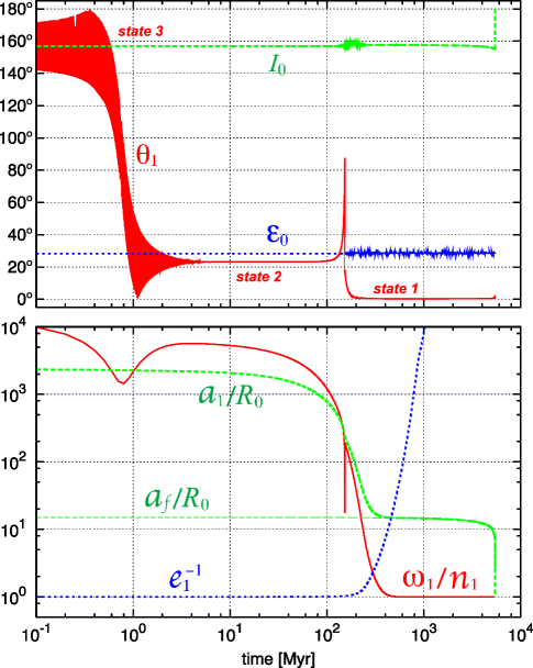
Figure 1.— Secular tidal evolution of the Triton-Neptune system. We plot the orbital inclination to the Laplacian plane $I_{0}$, the obliquity of Neptune to the ecliptic $\varepsilon_{0}$ and the obliquity of Triton to the orbital plane $\theta_{1}$ (top), and the semi-major axis ratios $a_{1}/R_{0}$ and $a_{f}/R_{0}$, the inverse of the eccentricity $e_{1}^{-1}$ and Triton’s rotation rate ratio $\omega_{1}/n_{1}$ (bottom).

As for the orbit, the initial spin of Triton is unknown. We tested several possibilities, but tides acting on the spin always drive it in the same way: the rotation rate quickly evolves into the equilibrium value given by equation (18), while the obliquity is trapped in Cassini state 2, for $\theta_{1}\simeq 180^{\circ}-I_{0}=23^{\circ}$ (Eq.21). In our standard simulation (Fig.1) we start Triton with a rotation period of 24 h and an obliquity $\theta_{1}=170^{\circ}$ (librating around Cassini state 3). In the very beginning, only Cassini states 2 and 3 exist ($\lambda_{1}\ll 1$), but according to equation (23), equilibrium in Cassini state 3 cannot be maintained (Fig.1a). As the semi-major axis decreases, the equilibrium obliquity for state 2 increases toward $90^{\circ}$ (Eq.21). At some point, the tidal torque becomes stronger than the conservative torque and the spin quits this state. The obliquity subsequently evolves into Cassini state 1 with $\theta_{1}\simeq I_{0}/\lambda_{1}$ (Eq.21). The orbital inclination to the Laplacian plane is more or less constant, but it presents some reduction when tides raised by Triton on Neptune become important (present day situation). At the very end of the evolution ($a_{1}\simeq 7.79$ $R_{0}$), this trend is reversed and the inclination quickly evolves into $180^{\circ}$. The obliquity of Neptune ($\varepsilon_{0}$) does not undergo any significant dissipation, but presents a secular oscillation of about one degree, from the moment Triton becomes an inner satellite ($a_{1}<100$ $R_{0}$). The semi-major axis and the eccentricity always decrease, as predicted by equations (26) and (27), and the quantity $a_{f}=a_{1}(1-e_{1}^{2})$ is preserved, during the first stages of the evolution, with the reduction observed being caused by tides on Neptune. The eccentricity is very high during the first evolutionary stages, decreasing very slowly. However, as soon as Triton becomes an inner satellite, the eccentricity quickly drops to a value very close to zero. Finally, the rotation of the satellite decreases as the satellite orbit shrinks into Neptune. It presents a rapid decrease when Cassini state 2 approaches $90^{\circ}$, explained by Eq. (18), and ultimately stabilizes in the synchronous resonance, the presently observed configuration.

5. Conclusion

We have shown that the tidal evolution of a satellite can only be correctly modeled when its spin is taken into account. Previous studies adopted synchronous motion from the very beginning, which is not the case for eccentric orbits. Tidal dissipation was therefore underestimated. With the same tidal parameters used by Goldreich et al. (1989) we are able to circularize Triton’s orbit in only 1 Gyr. Different tidal models and parameters may change the time-scale for the evolution, but the global picture should remain the same. We are also able to explain the present small value of Triton’s eccentricity $e_{1}\simeq 10^{-5}$, as well as its small obliquity $\theta_{1}=0.46^{\circ}$ and past evolution through Cassini states. In particular, we can exclude the possibility that Triton was initially captured in state 1 and determine when exactly the transition from state 2 to state 1 occurred (Chyba et al., 1989).

Our study should also apply to the Moon, Charon and the satellites of Mars, although in this case we need to take into account the quadropole moment of inertia $C_{22}\neq 0$ (Correia, 2006). It can also be easily generalized to other stellar systems.

The author thanks J. Laskar for helpful discussions. This work is dedicated to the memory of António and Nazareth Morgado.

References

- (1)
- Agnor and Hamilton (2006) Agnor C B and Hamilton D P 2006 Nature 441, 192–194.
- Anderson et al. (1998) Anderson J D, Schubert G, Jacobson R A, Lau E L, Moore W B and Sjogren W L 1998 Science 281, 2019–2022.
- Boué and Laskar (2006) Boué G and Laskar J 2006 Icarus 185, 312–330.
- Canup (2005) Canup R M 2005 Science 307, 546–550.
- Canup and Asphaug (2001) Canup R M and Asphaug E 2001 Nature 412, 708–712.
- Chyba et al. (1989) Chyba C F, Jankowski D G and Nicholson P D 1989 Astron. Astrophys. 219, L23–L26.
- Colombo (1966) Colombo G 1966 Astron. J. 71, 891–896.
- Correia (2006) Correia A C M 2006 Earth Planet. Sci. Lett. 252, 398–412.
- Correia and Laskar (2009) Correia A C M and Laskar J 2009 Icarus 201, 1–11.
- Cruikshank (1995) Cruikshank D P 1995 Neptune and Triton University of Arizona Press.
- Goldreich et al. (1989) Goldreich P, Murray N, Longaretti P Y and Banfield D 1989 Science 245, 500–504.
- Hut (1981) Hut P 1981 Astron. Astrophys. 99, 126–140.
- Jacobson (2009) Jacobson R A 2009 Astron. J. 137, 4322–4329.
- Kaula (1964) Kaula W M 1964 Rev. Geophys. 2, 661–685.
- Laplace (1799) Laplace P S 1799 Traité de Mécanique céleste Paris: Gauthier-Villars.
- McCord (1966) McCord T B 1966 Astron. J. 71, 585–590.
- McKinnon (1984) McKinnon W B 1984 Nature 311, 355–358.
- McKinnon and Leith (1995) McKinnon W B and Leith A C 1995 Icarus 118, 392–413.
- Mignard (1979) Mignard F 1979 Moon and Planets 20, 301–315.
- Mignard (1981) Mignard F 1981 Mon. Not. R. Astron. Soc. 194, 365–379.
- Néron de Surgy and Laskar (1997) Néron de Surgy O and Laskar J 1997 Astron. Astrophys. 318, 975–989.
- Peale (1969) Peale S J 1969 Astron. J. 74, 483–489.
- Pollack et al. (1979) Pollack J B, Burns J A and Tauber M E 1979 Icarus 37, 587–611.
- Schenk and Zahnle (2007) Schenk P M and Zahnle K 2007 Icarus 192, 135–149.
- Smart (1953) Smart W M 1953 Celestial Mechanics. London, New York, Longmans, Green.
- Stern and McKinnon (2000) Stern S A and McKinnon W B 2000 Astron. J. 119, 945–952.
- Thomas (2000) Thomas P C 2000 Icarus 148, 587–588.
- Tremaine et al. (2009) Tremaine S, Touma J and Namouni F 2009 Astron. J. 137, 3706–3717.
- Tsurutani et al. (1990) Tsurutani B T, Miner E D and Collins S A 1990 Earth and Space 3, 10–14.
- Vokrouhlický et al. (2008) Vokrouhlický D, Nesvorný D and Levison H F 2008 Astron. J. 136, 1463–1476.
- Ward and Hamilton (2004) Ward W R and Hamilton D P 2004 Astron. J. 128, 2501–2509.
- Yoder (1979) Yoder C F 1979 Nature 279, 767–770.
- Zhang and Hamilton (2008) Zhang K and Hamilton D P 2008 Icarus 193, 267–282.