Quantum Dynamics Against a Noisy Background

Abstract

By the example of a kicked quartic oscillator we investigate the dynamics of classically chaotic quantum systems with few degrees of freedom affected by persistent external noise. Stability and reversibility of the motion are analyzed in detail in dependence on the noise level $\sigma$. The critical level $\sigma_{c}(t)$, below which the response of the system to the noise remains weak, is studied versus the evolution time. In the regime with the Ehrenfest time interval $t_{E}$ so short that the classical Lyapunov exponential decay of the Peres fidelity does not show up the time dependence of this critical value is proved to be power-like. We estimate also the decoherence time after which the motion turns into a Markovian process.

Exponential sensitivity of nonlinear classical systems which display chaotic behavior to arbitrarily weak perturbations makes impractical the treatment of such systems as closed ones. Inevitably, the interaction with environment crucially influences the dynamics of such systems. In many cases this influence can be considered as a noise, that turns the motion into an irreversible random process.

Quite opposite, the quantum dynamics of the same systems manifests a considerable degree of stability against external perturbations arrow1 . A quantitative analysis shows arrow2 that the sensitivity to an instant perturbation is of a threshold nature: there exists a critical value $\xi_{c}$ of the strength $\xi$ of the perturbation, below which the response of the system remains weak. This critical value depends on complexity of the quantum Wigner function, that can be characterized, for example, by the number of its Fourier harmonics.

In general, the critical strength $\sigma_{c}(t)$ decreases exponentially within the Ehrenfest interval $0<t<t_{E}$ during which the Wigner function still satisfies the classical Liouville equation and therefore the role of the noisy environment remains decisive. This fact is very important Kolovsky94 for understanding the quantum-classical correspondence in the nontrivial case of classically chaotic systems. However, in the case when the Ehrenfest interval is so short that the classical exponential instability has not enough time to show up, in-depth information on chaotic quantum dynamics against a noisy background is quite limited up to now.

In this paper we present an advanced study of this problem. As in arrow2 , we use as a typical example the periodically kicked quartic oscillator whose one-step evolution is described by the Floquet operator ${\cal\hat{F}}=e^{-\frac{i}{\hbar}{\hat{H}}^{(0)}}\,{\hat{D}}\left(i\frac{g_{0}}{\sqrt{\hbar}}\right)=e^{-i\left(\omega_{0}{\hat{n}}+\hbar{\hat{n}}^{2}\right)}\,e^{i\frac{g_{0}}{\sqrt{\hbar}}\left({\hat{a}}+{\hat{a}}^{{\dagger}}\right)}$, where ${\hat{a}},{\hat{a}}^{{\dagger}}$ are the bosonic ($[{\hat{a}},{\hat{a}}^{{\dagger}}]=1$) creation-annihilation operators and ${\hat{n}}={\hat{a}}^{{\dagger}}{\hat{a}}$ is the excitation number operator. The driving force is given by $g(t)=g_{0}\sum_{\tau}\delta(t-\tau)$. The classical motion of this oscillator becomes chaotic when the kick strength $g_{0}$ exceeds unity. We suppose further that each kick is followed by an instant perturbation $\xi_{\tau}\,\hbar\,{\hat{n}}\delta(t-\tau)$ with Gaussian random intensity $\xi_{\tau}$, ($\langle\xi_{\tau}\rangle=0$, $\langle\xi_{\tau}\xi_{\tau^{\prime}}\rangle=\sigma^{2}\delta_{\tau\tau^{\prime}}$), which models a persistent external noise. Such a perturbation gives rise to the phase plane rotation by a random angle $\xi_{\tau}$ at the time moment $\tau$. For any given realization (history) $\{\xi\}\equiv\{\xi_{1},\xi_{2},...,\xi_{t}\}$ of the noise, the evolution is described by the unitary operator ${\hat{U}}(\{\xi\};t)=\prod_{\tau=1}^{\tau=t}\,\left[e^{-i\xi_{\tau}{\hat{n}}}\,{\cal\hat{F}}\right]$.

We consider below the time evolution of the initially pure state ${{\hat{\rho}}(0)=|0\rangle\langle 0|}$, where $|0\rangle$ is the ground eigenstate of the Hamiltonian ${\hat{H}}^{(0)}$. The corresponding quantum Wigner function $W(\alpha^{*},\alpha;0)=\frac{2}{\hbar}e^{-\frac{2}{\hbar}|\alpha|^{2}}$ is isotropic in the phase plane and occupies the phase cell $\hbar/2$. Few (one in the case of parameters chosen below) first kicks produce a state of a practically general form. At a running moment of time $t>0$, the excitation of the oscillator and the degree of anisotropy of the Wigner function are characterized by the probability distributions arrow2 ,

$$w_{n}(\{\xi\};t)=\langle n|{\hat{\rho}}(\{\xi\};t)|n\rangle\,,$$ (1)

and

$$\begin{array}[]{rl}\mathcal{W}_{m}(\{\xi\};t)&=(2-\delta_{m0})\sum_{n=0}^{\infty}\Big{|}\langle n+m\big{|}{\hat{\rho}}(\{\xi\};t)\big{|}n\rangle\Big{|}^{2}\\ &=(2-\delta_{m0})\sum_{n=0}^{\infty}w_{n}(\{\xi\};t)w_{n+m}(\{\xi\};t),\end{array}$$ (2)

respectively (both normalized to unity). Here ${\hat{\rho}}(\{\xi\};t)={\hat{U}}(\{\xi\};t){\hat{\rho}}(0){\hat{U}}^{{\dagger}}(\{\xi\};t)$. With the noise history being fixed, the evolution is unitary so that the state remains pure during the whole time of the motion.

Coarse-grained features of quantum evolution. The mean values $\langle n\rangle_{\{\xi\};t}$ and $\langle|m|\rangle_{\{\xi\};t}$ calculated with the help of the distributions (1,2) characterize respectively the degree of excitation and the number of $\theta$-harmonics, i.e. complexity arrow2 of the quantum state developed by the time $t$. Our numerical simulations showed that these values do not depend on the noise history at a given noise level $\sigma$ (i.e. they are self-averaging quantities).

As to the distributions (1,2) themselves, our detailed numerical data indicate (see upper panels in Fig.1; we fix system parameters as $\omega_{0}=1,\hbar=1,g_{0}=2$ throughout the paper; the Ehrenfest time $t_{E}<1$ in this case) that at a given time $t$ they undergo (as functions of $n$ or $m$, respectively) fluctuations, rather strong in the first case and much weaker in the second one, around a regular exponential decay with identical slopes. These slopes, contrary to the fluctuations, are not sensitive to the noise histories. Such universal exponential laws represent the coarse-grained distributions arrow2

$$w^{(c.g.)}_{n}(\sigma;t)=\frac{1}{\langle n\rangle_{\sigma;t}+1}\left[\frac{\langle n\rangle_{\sigma;t}}{\langle n\rangle_{\sigma;t}+1}\right]^{n},$$ (3)

and

$$\mathcal{W}^{(c.g.)}_{m}(\sigma;t)=\frac{2-\delta_{m0}}{2\langle|m|\rangle_{\sigma;t}+1}\left[\frac{\langle|m|\rangle_{\sigma;t}}{\langle|m|\rangle_{\sigma;t}+1}\right]^{m}$$ (4)

which entirely ignore the fluctuations. The first moments $\langle n\rangle_{\sigma;t}$ and $\langle|m|\rangle_{\sigma;t}=\langle n\rangle_{\sigma;t}$ of these distributions are the free parameters to be used for fitting the slopes of the actual distributions calculated numerically and plotted in Fig. 1. Being defined in such a way, they approximate quite well the corresponding history-insensitive mean values numerically found with the help of the exact distributions (3,4). Moreover, the analysis of our numerical data reveals (see the lower panels in Fig. 1) that the low moments depend very weakly on the noise level $\sigma$ as well. The chosen noise does not influence appreciably not only the number of harmonics but also the degree of excitation. Simulations with truncated excitation bases in the Hilbert space of different dimensions, $N\gg 1$ up to N=6000, convinced us that the rate of growth of the quantum mean excitation is practically indistinguishable from the classical diffusion law $\langle n\rangle_{t}=\frac{g_{0}^{2}}{\hbar}\,t$ (straight lines in lower panels in Fig. 1). Being in contrast to the case of the quantum kicked rotator, this fact agrees with the absence of localization of the eigenstates of the Floquet operator ${\cal\hat{F}}$ future . The increase of the number of angular harmonics $\langle m\rangle_{t}=\langle n\rangle_{t}$ is also linear as distinct from the classical exponential upgrowth. Furthermore, the amplitudes of fluctuations of the exact distributions (1,2) are appreciably reduced when the noise level $\sigma$ is growing.

A natural way of the coarse graining consists in averaging over realizations $\{\xi\}$ of the noise Sokolov84 . Indeed, as it follows from the data presented in Fig. 1, such an averaging leaves the slopes practically unchanged but suppresses the fluctuations. The latter are entirely obliterated at the strong noise limit $\sigma\rightarrow\infty$. Hence we define finally the coarse-grained distributions as

$$\begin{array}[]{c}w^{(c.g.)}_{n}(t)=\overline{w_{n}(\{\xi\};t)}\big{|}_{\sigma=\infty}=w^{(c.g.)}_{n}(\sigma=\infty;t);\\ \mathcal{W}^{(c.g.)}_{m}(t)=\overline{\mathcal{W}_{m}(\{\xi\};t)}\big{|}_{\sigma=\infty}=\mathcal{W}^{(c.g.)}_{m}(\sigma=\infty;t).\end{array}$$ (5)

The bar indicates averaging over the noise. Now, the connection $\langle|m|\rangle_{\infty;t}=\langle n\rangle_{\infty;t}$ directly follows from the exact relation (2) thus leading to the identity of the slopes. Being plotted, the coarse-grained distributions (3,4) are indistinguishable from the distributions (5) shown by the red/darkgray lines in Fig. 1.

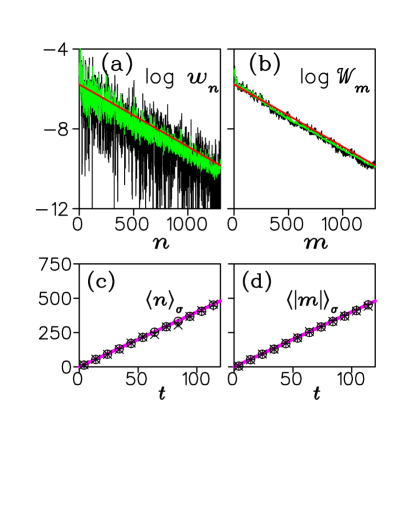
Figure 1: (Color online). (a),(b) - Probability distributions (1,2) at the moment $t=80$ with no noise ($\sigma=0$, black), weak noise ($\sigma=0.001$, green/gray) and in the strong noise limit, (red/darkgray) In the two latter cases the data have been averaged over $10^{3}$ noise realizations. (c),(d) - Time evolution of the moments $\langle n\rangle_{\sigma}$, $\langle|m|\rangle_{\sigma}$ (crosses, pluses and circles for $\sigma=0,0.001$ and $\sigma=\infty$, respectively) as compared to the classical diffusion law (straight magenta/gray lines).

The information entropy. As mentioned above, the characteristic number $\langle|m|\rangle_{\sigma;t}$ of harmonics of the Wigner function at a given moment of time $t$ can serve Brumer97 ; arrow2 as a measure of complexity of the current quantum state. Another possibility is to use Peres96 for the same purpose the information entropy. The latter, by virtue of the probabilistic interpretation, can be defined as

$${\cal I}(t) = -\sum_{m=0}^{\infty}\,\mathcal{W}^{(c.g.)}_{m}(t)\,\ln\mathcal{W}^{(c.g.)}_{m}(t)$$ (6)

$$\approx \ln\langle|m|\rangle_{\infty;t}+1+\frac{1}{2\langle|m|\rangle_{\infty;t}}+...\,,\,\,(t\gg 1).$$

This entropy grows monotonically with time starting from ${\cal I}(0)=0$. Generally speaking, during the Ehrenfest time $0<t\lesssim t_{E}$ the growth is linear with a slope determined by the classical Lyapunov exponent. Afterwards it slows down to the logarithmic behavior.

Sensitivity of quantum evolution to the noise. As usual, sensitivity of the motion to the noise could be characterized by the overlap (“fidelity”) $F(\{\xi\};t)=\mathrm{Tr}\left[{\hat{\rho}(t)}\,{\hat{\rho}(\{\xi\};t)}\right]$ of the states developed by the time $t$ during the evolution with or without influence of the noisy environment. However, contrary to the low moments of the distributions (1, 2), the quantity defined in such a way is not a self-averaging one and strongly depends on the noise history. The appropriate reduced measure is obtained by averaging over all possible noise realizations

$$F(\sigma;t) = \overline{F(\{\xi\};t)}$$ (7)

$$= \mathrm{Tr}\left[{\hat{\rho}(t)}\,{\hat{\rho}^{(av)}(\sigma;t)}\right]=\overline{\big{|}\langle 0|{\hat{f}}(\xi;t)|0\rangle\big{|}^{2}}\,.$$

The newly defined fidelity depends on the only parameter $\sigma$ instead of the entire noise history $\{\xi\}$. This definition brings into consideration the averaged density matrix ${\hat{\rho}^{(av)}(\sigma;t)}=\overline{{\hat{\rho}(\{\xi\};t)}}$ Zurek03 . Since

$$\langle n^{\prime}|{\hat{\rho}^{(av)}(\sigma;\tau)}|n\rangle=e^{-\frac{1}{2}\sigma^{2}(n^{\prime}-n)^{2}}\,\langle n^{\prime}|{\cal\hat{F}}{\hat{\rho}^{(av)}(\sigma;\tau-1){\cal\hat{F}}^{{\dagger}}}|n\rangle,$$ (8)

the averaging over the noise suppresses the off-diagonal matrix elements and cuts down the number of harmonics of the corresponding averaged Wigner function. Notice that the normalization condition ${\rm Tr}{\hat{\rho}^{(av)}(\sigma;\tau)}=1$ holds during the whole evolution independently of the noise level.

The unitary fidelity operator that appears in the r.h.s. of Eq. (7) reads

$${\hat{f}}(\{\xi\};t) = {\hat{U}}^{{\dagger}}(t)\,{\hat{U}}(\{\xi\};t)\equiv$$ (9)

$${{\cal\hat{F}}^{{\dagger}}}\,^{t}\,\prod_{\tau=1}^{\tau=t}\left[e^{-i\xi_{\tau}{\hat{n}}}\,{\cal\hat{F}}\right]=\prod_{\tau=1}^{\tau=t}e^{-i\xi_{\tau}{\hat{n}}(\tau)},$$

where ${\hat{n}}(\tau)={{\cal\hat{F}}^{{\dagger}}}\,^{\tau}{\hat{n}}\,{{\cal\hat{F}}}^{\,\tau}$ is the Heisenberg evolution of the operator ${\hat{n}}$. It is easy to calculate explicitly the fidelity (7) for the two limiting cases of weak and extremely strong noise.

Weak noise limit. Keeping in the last product the noise intensity $\xi_{\tau}\neq 0$ only in one certain exponential factor we reduce the problem to that considered in arrow2 . Averaging then over $\xi_{\tau}$, expanding up to the term $\thicksim\sigma^{2}$ and summing at last over all the moments $1\leq\tau\leq t$ we obtain

$$F(\sigma;t) = 1-\frac{1}{2}\sigma^{2}\sum_{\tau=1}^{\tau=t}\sum_{m=1}^{\infty}\,m^{2}\,\mathcal{W}_{m}(0;\tau)+O(\sigma^{4})=$$ (10)

$$1-\frac{1}{2}\sigma^{2}\sum_{\tau=1}^{\tau=t}\langle m^{2}\rangle_{0;\tau}+O(\sigma^{4})\,.$$

Therefore the fidelity stays close to unity while the noise level $\sigma$ remains appreciably below the critical value $\sigma_{c}(t)=\sqrt{2/\sum_{\tau=1}^{\tau=t}\langle m^{2}\rangle_{0;\tau}}\,.$ Insert in (Fig.2) demonstrates moderate decrease of fidelity during the first 100 kicks ($\hbar=1$). The classical Lyapunov decay does not show up. This quantum regime is opposed to the classical fast fall up to the same value in the case $\hbar=0.01$. Strictly speaking, the mean value $\langle m^{2}\rangle_{0;\tau}$ corresponds to the motion with no noise. However, as it has been already mentioned, the low moments of the harmonics distribution are practically insensitive to the noise so that $\langle m^{2}\rangle_{0;\tau}\approx\langle m^{2}\rangle_{\infty;\tau}=2\langle|m|\rangle^{2}_{\infty;\tau}=2\langle n\rangle^{2}_{\infty;\tau}\approx 2\left(\frac{g_{0}^{2}}{\hbar}\,\tau\right)^{2}$. This implies that $\sigma_{c}(t)\approx 1/\sqrt{\sum_{\tau=1}^{\tau=t}\langle|m|\rangle^{2}_{\infty;\tau}}\propto t^{-3/2}$. Though the critical value decreases with time faster than in the case of a single instant perturbation arrow2 , the decrease is power-like as before.

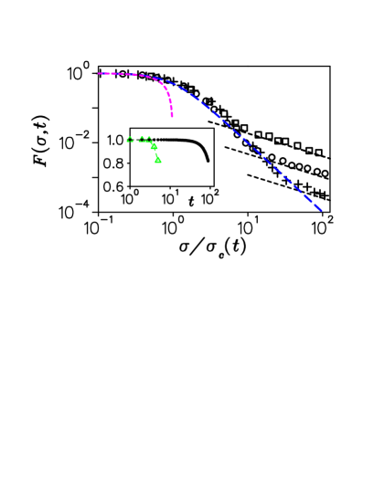
Figure 2: (Color online). The scaling properties of the fidelity. Crosses, circles and squares correspond respectively to: $\sigma=0.004,0.032$ and $0.256$. The magenta/grey and black short-dashed lines show the weak and strong noise limits (10) and (14); the blue/grey long-dashed line corresponds to the fit (15). Insert: fidelity decay in the classical Lyapunov ($\hbar=0.01$, green/gray triangles) and quantum ($\hbar=1$, black circles) regimes; in the both cases $\sigma=0,0005$. Notice logarithmic scale along the $t$ axis.

Strong noise limit. In the opposite case of extremely strong noise $\sigma\rightarrow\infty$ we insert $t$ times the completeness condition $\sum_{n=0}^{\infty}|n\rangle\langle n|=1$ while calculating the matrix element $f(\xi;t)\equiv\langle 0|{\hat{f}}(\xi;t)|0\rangle$, then calculate the average value $\overline{|f(\xi;t)|^{2}}$ and take at last into account that $\lim_{\sigma\rightarrow\infty}\,e^{-\frac{1}{2}\sigma^{2}m^{2}}=\delta_{m0}$. Finally we arrive at

$$\begin{array}[]{c}F_{\infty}(t)=\sum_{n_{t}}\big{|}\langle 0|{{\cal\hat{F}}^{\dagger}}\,^{\,t}|n\rangle\big{|}^{2}\sum_{n_{(t-1)}}\big{|}\langle n_{t}|{\cal\hat{F}}|n_{(t-1)}\rangle\big{|}^{2}\\ ...\sum_{n_{2}}\big{|}\langle n_{3}|{\cal\hat{F}}|n_{2}\rangle\big{|}^{2}\sum_{n_{1}}\big{|}\langle n_{2}|{\cal\hat{F}}|n_{1}\rangle\big{|}^{2}\big{|}\langle n_{1}|{\cal\hat{F}}|0\rangle\big{|}^{2}\,.\\ \end{array}$$ (11)

Only the transition probabilities in the absence of noise are present, the forward evolution being a chain of non-interfering successive transitions. Quite opposite, the backward transition contains the entire set of possible quantum-mechanical paths.

The evolution of the averaged density matrix is of special interest. Eq. (8) shows that in the strong noise limit the density matrix remains diagonal during the whole time of the motion: $\langle n^{\prime}|{\hat{\rho}^{(av)}(\infty;\tau)}|n\rangle\equiv\langle n^{\prime}|{\hat{\rho}^{(d)}(\tau)}|n\rangle=\delta_{n^{\prime}n}\,w^{(d)}_{n}(\tau)$. The evolution equation (8) reduces in this case to

$$w^{(d)}_{n}(\tau) = \sum_{n^{\prime}=0}^{\infty}\mathbb{Q}_{nn^{\prime}}\,w^{(d)}_{n^{\prime}}(\tau-1),$$ (12)

$$\mathbb{Q}_{nn^{\prime}} = \Big{|}\langle n|{\hat{D}}\left(i\frac{g_{0}^{2}}{\sqrt{\hbar}}\right)|n^{\prime}\rangle\Big{|}^{2}>0\,.$$ (13)

The matrix ${\hat{\mathbb{Q}}}$ is symmetric, positively definite, and obeys the condition $\sum_{n^{\prime}=0}^{\infty}\mathbb{Q}_{nn^{\prime}}=\langle n|n\rangle=1$. The equation (12) describes Lankaster69 a homogeneous Markov’s chain. Notice that the motion does not depend in this limit on the properties of the unperturbed Hamiltonian ${\hat{H}}^{(0)}.$

It immediately follows now that

$$F(\infty;t)=\sum_{n=1}^{\infty}w_{n}(0;t)\,w^{(d)}_{n}(t)\approx\frac{1}{2\langle n\rangle_{\infty;t}+1}\,.$$ (14)

We have used here the exponential ansatz (3) for both $w$ - distributions as well as the practical independence of the mean excitation number $\langle n\rangle_{\sigma;t}$ of the noise. This formula is in a good agreement with our numerical data.

Moderate noise: scaling property. Analytical consideration is not possible in the general case of the moderate noise level $\sigma\gtrsim\sigma_{c}(t)$. Generically, the evolution of the averaged density matrix ${\hat{\rho}}^{(av)}(\sigma;t)$ is not unitary. This entails state mixing and suppression of the quantum interference, i.e. decoherence. Nevertheless, even if this ratio exceeds unity, the fidelity (7) continues, as Fig. 2 clearly demonstrates, to depend only on the ratio $\sigma/\sigma_{c}(t)$ up to the time $t_{(dec)}(\sigma)$, when the full decoherence takes place and the evolution becomes Markovian.

A simple fit (compare with arrow2 )

$$F_{f}(\sigma;t)=\frac{1}{1+\sigma^{2}/\sigma_{c}^{2}(t)}\,,\quad t<t_{(dec)}(\sigma)$$ (15)

describes our numerical data rather well (Fig. 2). With the help of this fit, the decoherence time is estimated as $t_{(dec)}(\sigma)=\sqrt{\frac{6\hbar}{D\sigma^{2}}}$, where $D=g_{0}^{2}$ is the classical diffusion coefficient.

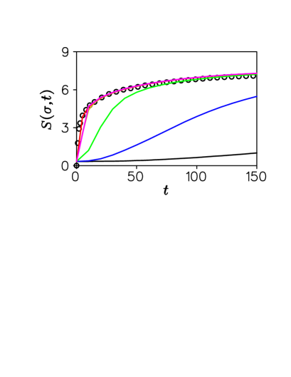
Figure 3: (Color online). Von Neumann entropy versus the time. From bottom to top (black, blue, green, magenta and red): $\sigma=(0.125,1,8,64,512)\cdot 10^{-3}$. Circles show the information Shennon entropy ${\cal I}(t)$, see eq. (6).

Loss of memory on the initial state. The state mixing induced by the noise leads to loss of memory about the initial state. Thereupon the notion of the invariant (independent of the basis) von Neumann entropy

$${\cal S}(\sigma;t)=-{\rm Tr}\left[{\hat{\rho}}^{(av)}(\sigma;t)\ln{\hat{\rho}}^{(av)}(\sigma;t)\right]$$ (16)

becomes relevant. This entropy increases with time monotonically, Fig. 3, approaching the function ${\cal I}(t)$ (6) from below when $t\rightarrow t_{(dec)}$. After the full decoherence takes place, the system occupies the whole phase volume accessible at the running degree of excitation $\langle n\rangle_{\sigma;t}\approx\langle n\rangle_{\infty;t}=\langle|m|\rangle_{\infty;t}$ thus reaching a sort of equilibrium. Henceforth the phase volume expands ”adiabatically”: the entropy ${\cal S}(\sigma;t>t_{(dec)})\approx{\cal I}(t)\approx\ln\langle|m|\rangle_{\infty;t}$ remains practically constant when $\langle n\rangle_{\infty;t}=\langle|m|\rangle_{\infty;t}\gg 1$. In particular case of the strong noise limit, $(\sigma\rightarrow\infty,\,t_{(dec)}\rightarrow 0)$, the averaged density matrix is diagonal and the von Neumann entropy equals

$$\begin{array}[]{rl}{\cal S}_{\infty}(t)&=-\sum_{n=0}^{\infty}w^{(d)}_{n}(t)\ln w^{(d)}_{n}(t)\\ &\approx\ln\langle n\rangle_{\infty;t}+1+\frac{1}{2\langle n\rangle_{\infty;t}}+...\,,\,\,\,\,(t\gg 1)\,.\\ \end{array}$$ (17)

We have arrived at a remarkable connection ${\cal S}_{\infty}(t)={\cal I}(t)$. Similar connection between the information and invariant von Neumann entropies has been discovered also in the theory of random band matrices Sokolov98 .

Reversibility versus Purity. Another interesting aspect of quantum motion under the influence of a noisy background is the degree of reversibility. This degree can naturally be measured by the mean overlap (Peres fidelity) of the initial state ${\hat{\rho}}(0)$ and the state ${\hat{\rho}}(0|\{\xi\},\{\xi^{\prime}\};t)$ formed during forward evolution for some time $t$ under the influence of a stationary noise with the level $\sigma$ and a history $\{\xi\}$ and then backward evolution for the same time under the same noise with an independent history $\{\xi^{\prime}\}$:

$$\begin{array}[]{rcl}\mathbb{F}(\sigma;t)=&\overline{\mathrm{Tr}\left[{\hat{\rho}}(0)\,{\hat{\rho}}(0|\{\xi\},\{\xi^{\prime}\};t)\right]}=&\\ &\overline{\mathrm{Tr}\left[{\hat{\rho}}(\{\xi\};t)\,{\hat{\rho}}(\{\xi^{\prime}\};t)\right]}=&\\ &{\rm Tr}\left[{\hat{\rho}}^{(av)}(\sigma;t)\,{\hat{\rho}}^{(av)}(\sigma;t)\right]&\equiv\mathbb{P}(\sigma;t)\,.\\ \end{array}$$ (18)

The quantity $\mathbb{P}(\sigma;t)$ is referred for as purity Zurek03 . It can be expressed in terms of the mean number of harmonics $\langle|{\mathfrak{m}}|\rangle_{\sigma;t}$ of the averaged Wigner function. The corresponding probability distribution is related to the averaged density matrix ${\hat{\rho}}^{(av)}(\sigma;t)$ as

$$\mathbb{W}_{m}(\sigma;t)=(2-\delta_{m0})\frac{\sum_{n=0}^{\infty}\Big{|}\langle n+m\big{|}{\hat{\rho}}^{(av)}(\sigma;t)\big{|}n\rangle\Big{|}^{2}}{\mathbb{P}(\sigma;t)}\,.$$ (19)

(to be confronted with eq.(2)). This means in particular that, in the exponential approximation for mixed states arrow2 ,

$$\mathbb{P}(\sigma;t) = \frac{1}{\mathbb{W}_{0}(\sigma;t)}\sum_{n=0}^{\infty}\left[w^{(av)}_{n}(\sigma;t)\right]^{2}\approx$$ (20)

$$\frac{2\langle|{\mathfrak{m}}|\rangle_{\sigma;t}+1}{2\langle n\rangle_{\sigma;t}+1}\xrightarrow{\sigma\rightarrow\infty}\frac{1}{2\langle n\rangle_{\infty;t}+1}\,.$$

Contrary to $\langle|m|\rangle_{\sigma;t}$, the mean value $\langle|{\mathfrak{m}}|\rangle_{\sigma;t}$ strongly depends on the noise level and vanishes rapidly when $\sigma$ grows. Comparison with Eq. (14) shows that, as in arrow2 , the degrees of reversibility and sensitivity to external perturbations are directly connected, $\mathbb{F}(\infty;t)=F(\infty;t)$. Notice also the relation ${\cal S}_{\infty}(t)\approx-\ln\mathbb{P}_{\infty}(t),\,(t\gg 1)$ that follows from Eqs. (17,20).

Summary. The main goal of this Letter was to investigate in detail the the dynamics of a classically chaotic quantum system with few (one in our illustrative model) degrees of freedom affected by a persistent external noise under the condition that the Ehrenfest time interval is so short that the classical-like exponential instability does not show up. We have shown first that the noise weakly influences the complexity of the quantum state, which we characterize by the mean number $\langle|m|\rangle_{\sigma;t}$ of $\theta$-harmonics of the Wigner function. This number almost does not depend on the noise realization (self-averaging property) as well as on the level of the noise. At the same time the noise efficiently washes off fluctuations of the corresponding probability distribution thereby displaying the universal regular exponential decay of the coarse-grained distribution that describes the features of the motion independent of the realization of the noise.

The Peres fidelity that specifies a quantitative measure of sensitivity of the motion to the noise utilizes the density matrix ${\hat{\rho}}^{(av)}(\sigma;t)$ averaged over the noise. The sensitivity remains weak until the noise level $\sigma$ exceeds some critical value. We have proved that with the assumptions indicated above the decrease of this critical value is power-like, $\sigma_{c}(t)\approx 1/\sqrt{\sum_{\tau=1}^{\tau=t}\langle|m|\rangle^{2}_{\infty;\tau}}\propto t^{-3/2}$.

A scaling behavior has been discovered: the Peres fidelity depends only on the ratio $\sigma^{2}/\sigma_{c}^{2}(t)$ in a wide interval of the noise level up to some value $\sigma_{d}(t)$ that is considerably larger than the critical value $\sigma_{c}(t)$. The scaling is destroyed only under influence of even a stronger noise $\sigma>\sigma_{d}(t)$. The evolution becomes Markovian in this case. This implies that decoherence takes place at the time $t_{(dec)}(\sigma)\thicksim\sqrt{\frac{\hbar}{D\sigma^{2}}}$. The information entropy and the invariant von Neumann entropy coincide, ${\cal S}_{\sigma}(t)\Rightarrow{\cal I}(t)$, when $t\gtrsim t_{(dec)}(\sigma)$. They are identical in the limit $\sigma\rightarrow\infty$. We have also noticed that the reversibility of the motion influenced by a persistent noise is measured by the purity of the state at the moment of time reversal, $\mathbb{F}(\sigma;t)=\mathbb{P}(\sigma;t)$.

References

(1)
D.L. Shepelyansky, Physica D 8, 208 (1983); G. Casati,
B.V. Chirikov, I. Guarneri, and D.L. Shepelyansky, Phys. Rev.
Lett. 56, 2437 (1986).
(2)
V.V. Sokolov and O.V. Zhirov, EPL 84 30001 (2008); V.V.
Sokolov, O.V. Zhirov, G. Benenti, G. Casati, Phys. Rev. E 78 (046212) (2008) (see also in: ”Topics on Chaotic Systems:
Selected Papers from CHAOS2008 International Conference“,
World Scientific, (314-322) (2009)); G. Benenti, G. Casati,
Phys. Rev. E 79 025201(R) (2009).
(3)
A. Kolovsky, Europhys. Lett. 27 79 (1994); CHAOS 6
534 (1996); S. Habib, K. Shizume, W.H. Zurek, Phys. Rev. Lett.
80 4361 (1998).
(4) Oleg V. Zhirov, Valentin V. Sokolov, Yaroslav A. Kharkov,
in preparation