On the Degrees of Freedom of Finite State Compound Wireless Networks - Settling a Conjecture by Weingarten et. al.

Abstract

We explore the degrees of freedom (DoF) of three classes of finite state compound wireless networks in this paper. First, we study the multiple-input single-output (MISO) finite state compound broadcast channel (BC) with arbitrary number of users and antennas at the transmitter. In prior work, Weingarten et. al. have found inner and outer bounds on the DoF with 2 users. The bounds have a different character. While the inner bound collapses to unity as the number of states increases, the outer bound does not diminish with the increasing number of states beyond a threshold value. It has been conjectured that the outer bound is loose and the inner bound represents the actual DoF. In the complex setting (all signals, noise, and channel coefficients are complex variables) we solve a few cases to find that the outer bound – and not the inner bound – of Weingarten et. al. is tight. For the real setting (all signals, noise and channel coefficients are real variables) we completely characterize the DoF, once again proving that the outer bound of Weingarten et. al. is tight. We also extend the results to arbitrary number of users. Second, we characterize the DoF of finite state scalar (single antenna nodes) compound $X$ networks with arbitrary number of users in the real setting. Third, we characterize the DoF of finite state scalar compound interference networks with arbitrary number of users in both the real and complex setting. The key finding is that scalar interference networks and (real) $X$ networks do not lose any DoF due to channel uncertainty at the transmitter in the finite state compound setting. The finite state compound MISO BC does lose DoF relative to the perfect CSIT scenario. However, what is lost is only the DoF benefit of joint processing at transmit antennas, without which the MISO BC reduces to an $X$ network.

1 Introduction

Recent advances in network information theory – such as the idea of interference alignment – have greatly widened the gap between the theoretical capacity predictions of wireless networks and the achievable rates with currently known practical schemes. The large gap is reminiscent of the early days of information theory when Shannon showed the theoretical capacity of a point to point channel to be far beyond what was then thought achievable. The gap between theory and practice, both then and now, can be viewed as a debate between structured and random coding approaches. Remarkably, both theory and practice have switched sides on the issue of random versus structured codes. When Shannon theory advocated random coding, practical schemes were exclusively focused on structured codes that could be decoded with a reasonable complexity. That debate was essentially won by theory as practical schemes like turbo codes were found to mimic random coding schemes and thereby approach theoretical limits with reasonable complexity. In the new debate, the situation is reversed. Recent theoretical advances advocate highly sophisticated structured codes while the achievable rates considered practical draw largely on basic random coding arguments. In the new debate it is not at all clear if theory will emerge as the winner. The issue separating theory and practice is no longer merely a matter of complexity at the receivers. Rather, it is not known whether theoretical results that support structured codes based on idealized assumptions such as perfect – and sometimes global – channel knowledge at the transmitters, will be robust to channel uncertainty, at least to the extent that it is fundamentally unavoidable in wireless networks. Since many of these recent theoretical insights emerge out of the degrees of freedom (DoF) perspective, a natural question is to explore the robustness of the DoF results to channel uncertainty at the transmitters.

It is well known that the MIMO point to point channel and the MIMO multiple access channel do not lose any DoF due to the lack of channel state information at the transmitters (CSIT). Evidently, this is because the combination of joint processing of all received signals and perfect channel state information at the receiver (CSIR) is able to compensate for the lack of CSIT. However, for most other MIMO networks the DoF are not believed to be robust to channel uncertainty at the transmiter. Consider, for example, the MIMO broadcast channel with $M$ antennas at the transmitter and $N_{1},N_{2}$ antennas at the two receivers. With perfect channel knowledge this channel has a total of $\min(M,N_{1}+N_{2})$ DoF [1], which is the same as with perfect cooperation at the receivers. However, in the ergodic time-varying i.i.d. Rayleigh fading case for example, it is known that with no CSIT, the MIMO broadcast channel loses DoF to the extent that time-division between users is optimal [2] for all points in the DoF region. For the two user MIMO interference channel with $M_{1},M_{2}$ antennas at the two transmitters and $N_{1},N_{2}$ antennas at their corresponding receivers, the DoF with perfect CSIT are characterized in [1] as $\min(M_{1}+M_{2},N_{1}+N_{2},\max(M_{1},N_{2}),\max(M_{2},N_{1}))$. With no CSIT the loss of DoF is characterized in [2]. Interestingly, the loss of DoF is shown to depend on the relative number of antennas at the transmitters and receivers. For example, if the transmitters have at least as many antennas as their desired receivers, $M_{1}\geq N_{1},M_{2}\geq N_{2}$, then DoF are lost to the extent that simple time-division between the two users achieves all points in the DoF region. On the other hand, if the receivers have at least as many antennas as their interfering transmitters, i.e. $N_{1}\geq M_{2},N_{2}\geq M_{1}$ then there is no loss of DoF due to the absence of CSIT. As in the multiple access channel, concentration of antennas at the receivers allows the benefits of joint signal processing under perfect channel knowledge, which is sufficient to offset the limitations of no CSIT for the entire DoF region. However, for most networks where the antennas are not disproportionately located on the receivers – such as networks of single antenna nodes – the DoF penalty due to the total lack of CSIT can be quite severe. For example, under the i.i.d. fading assumption (independent identically distributed across all dimensions), any distributed network of single antenna nodes has only 1 DoF in the absence of CSIT. This is because all received signals are statistically equivalent and therefore any receiver can decode all the messages. Since a receiver with only 1 antenna can decode all messages, the sum DoF cannot be more than 1. The DoF loss due to lack of CSIT is very significant for larger networks because with full CSIT these networks have been shown to be capable of much higher DoF. For example, an interference network with $K$ transmitter-receiver pairs is shown to have $K/2$ DoF in [3], and an $X$ network with $S$ source nodes and $D$ destination nodes is shown to have $\frac{SD}{S+D-1}$ DoF in [4]. Evidently, the transmitters’ ability to exploit the channel structure to selectively align signals – the key to the DoF of interference and $X$ networks – is lost when CSIT is entirely absent.

While perfect CSIT is an overly optimistic assumption, the complete lack of CSIT is overly pessimistic. The collapse of DoF in the total absence of CSIT, while sobering, is not a comprehensive argument against the potential benefits of interference alignment in particular or structured coding approaches in general. Hence the need to investigate the behavior of DoF under partial channel knowledge. Two kinds of approaches have been followed in this regard.

The first approach investigates how the quality of CSIT should improve as SNR increases, in order to retain the same DoF as possible with perfect CSIT. A representative work that takes the first approach is [5] where the two user MISO BC is investigated under the assumption that the channel vector of one user (say user 1) is known perfectly but the channel vector of the other user (user 2) can take one out of two values. The angular separation $\theta$ between the two possible channel vectors of user 2 is chosen as a measure of the channel uncertainty and it is investigated how $\theta$ should diminish as SNR approaches infinity in order to retain the full (two) DoF possible with perfect CSIT. It is shown that $\sin^{2}(\theta)=O(\mbox{SNR}^{-1})$ is required to achieve two DoF in this setting. Other related works that follow this approach include [6, 7, 8].

The second approach seeks the impact on DoF of a fixed amount of channel uncertainty that is independent of SNR. References [9, 10] take this approach for the two user MISO BC. While [9] assumes channel uncertainty over a space of non-zero probability measure under time-varying channel conditions, [10] investigates a finite state compound channel setting where a specific channel state is drawn (unknown to the transmitter) from a finite set of allowed states and the chosen state is held fixed throughout the duration of communication. As large as this set may be, its finite cardinality restricts the channel uncertainty at the transmitter to a space of zero measure. While the two settings are quite different, the conclusions arrived at in [9] and [10] bear striking similarities. For example, with $M=2$ antennas at the transmitter, the best outer bound on the DoF in both works is equal to $\frac{4}{3}$. In both works it is conjectured that this outer bound is loose in general. Lapidoth et. al. [9] conjecture that the DoF in their setting should collapse to 1. Remarkably, Weingarten et. al. [10] show the achievability of $\frac{4}{3}$ DoF when each user’s channel can be in one of two states. However, as the number of possible channel states for either user (or both users) increases, Weingarten et. al. [10] also conjecture that the DoF in their setting should collapse to 1. Our main contribution in this paper is to settle the latter conjecture in the negative.

The central concept involved in this work – as well as in the original work of Weingarten et. al. [10] – is the idea of interference alignment, i.e. structuring signals in such a way that undesired signals cast overlapping shadows where they are not desired while they remain distinguishable where they are desired. The idea originated out of the study of the $2$ user $X$ channel [11, 12, 13]. The benefits of overlapping interference spaces were first pointed out in the context of the 2 user $X$ channel in [11, 12] and the concept of interference alignment was crystallized in [13], where the first linear (based on beamforming/zero-forcing over extended channel symbols) interference alignment scheme was introduced. [11, 12] established the achievability of $\lfloor\frac{4}{3}M\rfloor$ DoF for the $2$ user $X$ channel where all nodes are equipped with $M$ antennas each. For the same channel model, [13] derived the outer bound, DoF $\leq\frac{4}{3}M$, and also proved its achievability for $M>1$. For $M=1$ (single antenna at all nodes), [13] showed the achievability of $\frac{4}{3}$ DoF only for a time-varying/frequency-selective channel model. Achievability of $\frac{4}{3}$ DoF for the constant (not time-varying or frequency-selective) channel case, with complex channel coefficients, was established in [14] where the idea of asymmetric complex signaling was introduced to achieve interference alignment. The constant channel case with real channel coefficients was studied in [15]. Building on the idea of alignment of lattices scaled by rational/irrational factors, originally introduced in [16], it was shown by [15] that the outer bound of $\frac{4}{3}$ DoF is also achievable when the channel coefficients are real. All these ideas – zero-forcing, beamforming, channel extensions, asymmetric complex signaling, rational/irrational scaled lattice alignment – are used for the achievable schemes in this paper. In addition, we make use of the interference alignment schemes used for the SIMO interference channel in [17], which turns out to be the dual/reciprocal network for the compound MISO BC. An interesting outcome of this duality perspective is to clarify the role of alignment of vector spaces at the transmitter instead of the receivers.

A striking observation from the results summarized above, is the recurrence of the fraction $\frac{4}{3}$ in the DoF characterizations of both the 2 user $X$ channel, as well as the compound MISO BC. As we find in this work, this is not merely a coincidence. With enough channel uncertainty, the finite state compound BC – regardless of the number of users or transmit antennas – loses the DoF benefits of joint signal processing at the transmitter. From the DoF perspective, this makes the finite state compound MISO BC equivalent to a finite state compound $X$ channel. Moreover, the finite state compound $X$ channel does not lose any DoF compared to the perfect CSIT scenario (non-compound setting). Thus, the DoF of the compound MISO BC end up being equal to the DoF of the $X$ channel obtained by separating the transmit antennas. Similar to $X$ networks, we find that $K$ user interference networks also do not lose DoF in the finite state compound channel setting. It should be noted that some of these results are found in the real setting, i.e. all channel coefficients and signals and noise are restricted to take only real values.

We present the system model in the next section. The main results are presented as theorems in Section 2 and 3 along with the main ideas needed for the proofs. The detailed proofs are presented in the Appendix and the conclusions are summarized in Section 7.

2 Compound MISO Broadcast Channel - Complex Setting

A compound MISO broadcast channel consists of a transmitter with $M>1$ antennas and $K$ single antenna receivers. The channel vector $\mathbf{h}^{[k]}$ associated with user $k$ is drawn from a set $\mathcal{J}_{k}$ with finite cardinality $J_{k}$. To avoid degenerate cases, we assume the channel states are drawn from a continuous distribution. Thus, almost surely the channel states are generic, e.g., the coefficients are algebraically independent. Once the channel is drawn, it remains unchanged during the entire transmission. While the transmitter is unaware of the specific channel state realization, the receivers are assumed to have perfect channel knowledge. The transmitter sends independent messages $W^{[k]}$ with rates $R^{[k]}$ to receiver $k=1,2,\ldots,K$, respectively. A rate tuple $(R^{[1]},R^{[2]},\ldots,R^{[K]})$ is achievable if each receiver is able to decode its message with arbitrary small error probability regardless of state (realization) of the channel. The received signal of user $k$ corresponding to channel state index $j_{k}$ is given by

$$y^{[k]}_{j_{k}}(n)=\mathbf{h}^{[k]}_{j_{k}}{\bf x}(n)+z^{[k]}_{j_{k}}(n)~{}~{}~{}~{}k=1,\ldots,K~{}~{}j_{k}=1,\ldots,J_{k}$$ (1)

$\mathbf{h}^{[k]}_{j_{k}}=\left[h_{j_{k}1}^{[k]},\ldots,h_{j_{k}M}^{[k]}\right]$ is a $1\times M$ channel vector between the transmitter and receiver $k$ under state $j_{k}$ where $j_{k}\in\{1,\ldots,J_{k}\}$. $\mathbf{x}=\left[x_{1}(n),\ldots,x_{M}(n)\right]^{T}$ is an $M\times 1$ transmitted complex vector at time $n$ and satisfies the average power constraint $E(\|\mathbf{x}\|^{2})\leq P$. $z^{[k]}_{j_{k}}$ represents independent identically distributed (i.i.d.) zero mean unit variance circularly symmetric complex Gaussian noise. The total number of degrees of freedom $d$ is defined as

$$d=\lim_{P\rightarrow\infty}\frac{R^{[1]}+\cdots+R^{[K]}}{\log P}$$ (2)

A two user compound broadcast channel with $M=2,J_{1}=J_{2}=J=2$ is shown in Figure 1.

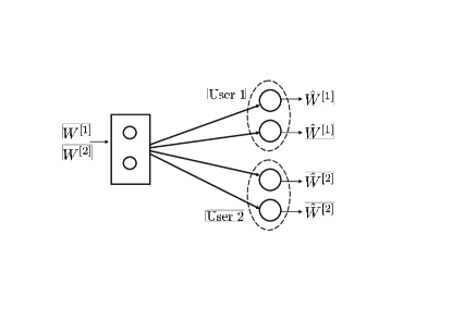
Figure 1: $2$ User Compound Broadcast Channel with $J_{1}=J_{2}=2$

Remark: The compound broadcast channel is equivalent to a broadcast channel with common messages. This can be seen by considering different states as different users. Now instead of a $K$ user compound broadcast channel, we have a $J_{1}+\cdots+J_{K}$ user broadcast channel with $K$ common messages, one for each group $k,\forall k=1,\ldots,K$, with $J_{k}$ users.

2.1 Degrees of Freedom of the Complex Compound MISO BC

The degrees of freedom of the complex compound MISO BC are studied by Weingarten, Shamai and Kramer in [10]. The exact DoF are found for some cases and conjectures are made for more general scenarios. The achievability of the conjectured DoF is established in [10]. We start with the first conjecture, re-stated here in the terminology of our system model.

Case 1: $J_{1}=1,J_{2}=J\geq M$

Conjecture 1

(Weingarten et. al. [10]) Consider a complex compound BC with $K=2$ users, $M$ antennas at the transmitter, and $J_{1}=1,J_{2}=J\geq M$ possible generic states for users 1,2 respectively. Then the total number of DoF is $1+\frac{M-1}{J}$, almost surely.

Consider the MISO BC with 2 antennas at the transmitter. The case of perfect CSIT corresponds to $J_{1}=J_{2}=1$. In this case it is easy to see that 2 DoF can be achieved by zero forcing at the transmitter. Specifically, the transmitter beamforms to user 1 in a direction orthogonal to the channel vector of user 2, and beamforms to user 2 in a direction orthogonal to the channel vector of user 1. Since neither user sees interference, they are able to achieve 1 DoF each.

Now, let us introduce some channel uncertainty with $J_{1}=1,J_{2}=J=2$, i.e. user 1’s channel is perfectly known to the transmitter but user 2’s channel can take one out of two known values. In this case it is clear that the transmitter can still choose a beamforming direction to user 2 that is orthogonal to the known channel vector of user 1. However, it is not possible to pick a beamforming vector for user 1 that is orthogonal to both the possible channel vectors of user 2. This is because the transmitter has only 2 antennas and the two possible channel vectors of user 2 span the entire two dimensional transmit space available to the transmitter. It is shown by Weingarten et. al. [10] that the best thing to do in this setting, from a DoF perspective, is to choose the beamforming vector for user 1 to be orthogonal to the first possible channel vector of user 2 for half the time and then choose it to be orthogonal to the second possible channel vector of user 2 for the remaining half of the time. In this manner, regardless of his state, user 2 is able to see an interference free channel for half the time, thus achieving 0.5 DoF. At the same time, user 1 sees no interference from user 2’s signal and is able to achieve 1 DoF. Thus a total of $\frac{3}{2}$ DoF is achieved. Following the same idea, one can achieve $1+\frac{M-1}{J}$ DoF for general values of $M,J$. Interestingly, when $J$ is equal to $M$, [10] shows that this is optimal. Thus the compound BC loses DoF relative to the perfect CSIT setting. For $J>M$ it is conjectured that $1+\frac{M-1}{J}$ is still optimal. Note that if this conjecture were to be true, this would mean that the DoF of the MISO BC collapse to $1$ as the number of channel states of either user increases.

To disprove this conjecture, we provide a specific counter example in the following theorem.

Theorem 1

For the complex compound MISO BC with $K=2$ users, $M=2$ antennas at the transmitter and $J_{1}=1$, $J_{2}=J=3$ generic channel states for users $1,2$ respectively, the exact number of total DoF = $\frac{3}{2}$, almost surely.

Since $1+\frac{M-1}{J}=\frac{4}{3}<\frac{3}{2}$ in this case, Conjecture 1 is disproved by Theorem 1. Interestingly, Theorem 1 indicates that the total number of DoF does not decrease even as the number of possible channel states for user 2 increases from 2 to 3. The reason we are able to achieve more than the conjectured DoF in this case, can be attributed to interference alignment schemes inspired by recently developed insights on asymmetric complex signaling [14], and a reciprocity/duality relationship with the interference alignment problem for SIMO interference channels [17] that offers a clear perspective of interference alignment at the transmitter.

Asymmetric complex signaling involves reducing the complex setting to a real setting by treating a complex number as a two dimensional vector with real elements. In this setting, the scenario of Theorem 1 can be seen as a transmitter with $4$ antennas, while each receiver has two antennas. Very importantly, this mapping to the real setting introduces some structure in the channel as complex channel coefficients are translated to quaternionic matrix forms. Because of this structure the proof of Theorem 1 involves some subtleties that may distract from the main concept behind the interference alignment. For simplicity of exposition, we defer the fine details of the proof to Appendix A and highlight the main concepts in this section. Specifically, in the following explanation we ignore the special structure of the channel matrices and treat them as generic MIMO channels between a $4$-antenna transmitter and $2$-antenna receivers.

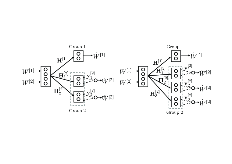
Figure 2: $2$ user compound MIMO BC with $J_{1}=1,J_{2}=2$ and $J_{1}=1,J_{2}=3$

As mentioned before, the 2 user compound MIMO BC is equivalent to a MIMO BC with two common messages, one for each of the two groups. Group $k=1,2,$ consists of $J_{k}$ users corresponding to $J_{k}$ states of user $k$ in the compound BC, and the users in the same group need to decode the same message (see Figure 2). Since there is only one receiver in group 1, we omit the index $j_{1}$ and replace $j_{2}$ with $j$ for simplicity. In addition, we use ${\bf H}^{[1]},{\bf H}_{j}^{[2]}$ to denote the channel matrix from the transmitter to user 1 (group 1) and receiver $j$ in group 2, respectively.

Consider first, an alternate achievable scheme for the case of $J_{1}=1,J_{2}=2$. We let the two receivers in group 2 use arbitrarily picked combining column vectors ${\bf v}_{1}^{[2]}$ and ${\bf v}_{2}^{[2]}$, respectively, along which they require interference free reception in order to achieve 1 DoF for their desired message. In order to protect these group 2 receivers, the transmitter sends user 1’s message along the directions orthogonal to ${\bf v}_{1}^{[2]T}{\bf H}_{1}^{[2]}$ and ${\bf v}_{2}^{[2]T}{\bf H}_{2}^{[2]}$. Since the transmitter has $4$ antennas – i.e., a $4$ dimensional transmit signal space – it is able to find a two dimensional subspace that is orthogonal to the protected dimensions of user $2$. This allows $2$ real streams to be sent to receiver 1 that do not interfere with the chosen directions of any of the receivers in group 2. On the other hand user 2’s message will be sent along the null space of ${\bf H}^{[1]}$. Since this is a rank $2$ matrix, it also has a two dimensional null space along which user 2’s message can be transmitted. However, because each of group 2 receivers have chosen only one receive dimension, only one interference free stream is sent. Thus, a total of $3$ interference free streams are delivered (2 streams to user 1 and 1 stream to every receiver of group 2). Since these are real signals, the total DoF achieved is $\frac{3}{2}$.

Now consider the case $J_{2}=3$. Suppose the third user in group 2 chooses a combining vector ${\bf v}_{3}^{[2]}$ for its interference-free desired signal dimension. Now in order to protect the chosen dimensions of group 2 receivers, the signals for user 1 should be transmitted orthogonal to the three $1\times 4$ vectors ${\bf v}_{1}^{[2]T}{\bf H}_{1}^{[2]}$, ${\bf v}_{2}^{[2]T}{\bf H}_{2}^{[2]}$ and ${\bf v}_{3}^{[2]T}{\bf H}_{3}^{[2]}$. Without alignment these three vectors will span a three dimensional space that needs to be protected from user 1’s signal, leaving only 1 dimension at the transmitter to send user 1’s message. However, we wish to allow user 1 to still access 2 interference-free dimensions. To achieve this goal, we need to make these three vectors span only a two dimensional vector subspace as seen by the transmitter, i.e. the three vectors should be linearly dependent. Equivalently, three column vectors ${\bf H}_{1}^{[2]T}{\bf v}_{1}^{[2]},{\bf H}_{2}^{[2]T}{\bf v}_{2}^{[2]},{\bf H}_{3}^{[2]T}{\bf v}_{3}^{[2]}$ should be linearly dependent. Since ${\bf H}_{1}^{[2]T}$, ${\bf H}_{2}^{[2]T}$ and ${\bf H}_{3}^{[2]T}$ are three $4\times 2$ generic matrices, the column spaces of any two of the three matrices only have null intersection, almost surely. In other words, any two of ${\bf H}_{1}^{[2]T}{\bf v}_{1}^{[2]},{\bf H}_{2}^{[2]T}{\bf v}_{2}^{[2]}$ and ${\bf H}_{3}^{[2]T}{\bf v}_{3}^{[2]}$ cannot be aligned along the same direction. Therefore, we align the vector ${\bf H}_{3}^{[2]T}{\bf v}_{3}^{[2]}$ in the space spanned by ${\bf H}_{1}^{[2]T}{\bf v}_{1}^{[2]}$ and ${\bf H}_{2}^{[2]T}{\bf v}_{2}^{[2]}$. Mathematically, we have

$${\bf H}_{3}^{[2]T}{\bf v}_{3}^{[2]}\in\textrm{span}([{\bf H}_{1}^{[2]T}{\bf v}_{1}^{[2]}~{}{\bf H}_{2}^{[2]T}{\bf v}_{2}^{[2]}])$$ (3)

The above alignment is the key to achieving more than the conjectured DoF in this case. Whereas most interference-alignment schemes [3, 4, 13, 14] align interfering dimensions in a one-to-one fashion, this is impossible in this case as pointed above. What is needed instead, is an alignment of an interfering dimension within the space spanned by several others. As it turns out, this problem bears a striking resemblance to the interference alignment scheme used in [17] for the MIMO interference channel where the interference vectors from one interferer are aligned in the space spanned by the interference vectors of other interferers.

To illustrate the concept with an example, let us consider a $4$ user many-to-one interference network with $2$ antennas at each transmitter and $4$ antennas at each receiver (see Figure 3). We claim user 1 can achieve $2$ DoF and other users achieve 1 DoF simultaneously. Let ${\bf H}^{[ji]}$ denote the $4\times 2$ channel from transmitter $i$ to receiver $j$,${\bf V}^{[1]}$ denote the $2\times 2$ beamforming matrix for transmitter 1 and ${\bf v}^{[i]}$ denote the $2\times 1$ beamforming vectors of transmitter $i=2,3,4$. Choose ${\bf v}^{[4]}$ randomly and let

$$\left[\begin{array}[]{c}{\bf v}^{[2]}\\ {\bf v}^{[3]}\end{array}\right]={\left[{\bf H}^{[12]}~{}{\bf H}^{[13]}\right]}^{-1}{\bf H}^{[14]}{\bf v}^{[4]}\Rightarrow{\bf H}^{[14]}{\bf v}^{[4]}\in span(\left[{\bf H}^{[12]}{\bf v}^{[2]}~{}{\bf H}^{[13]}{\bf v}^{[3]}\right])$$ (6)

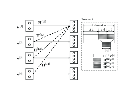
Figure 3: $4$ user many-to-one interference network with 2 antennas at transmitter, 4 antennas at receiver

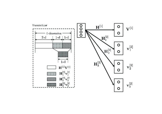
Figure 4: $2$ compound broadcast channel with 4 antennas at transmitter, 2 antennas at receiver, and $J_{1}=1,J_{2}=J=3$

Since receivers $2$ to $4$ are interference free they can decode their own message successfully. Now consider receiver 1. The spaces spanned by the column vectors of ${\bf H}^{[12]}$ and ${\bf H}^{[13]}$ only have null intersection. Thus the interference from user $2$ and $3$ together occupies $2$ dimensions – i.e., it does not align. For the same reason, the interference from user 4 can also not be aligned within the one dimensional interference from user 2 or from user 3, individually. However, the interference from user $4$ is aligned in the 2 dimensional subspace space spanned by interference from user $2$ and $3$ together. Thus, receiver $1$ sees $4-2=2$ interference free dimensions for its intended signal vectors. Comparing Figure 4 with Figure 3, the only difference is that the signal spaces are aligned at the transmitter for compound broadcast channel while they are aligned at the receiver for many-to-one interference channel. In other words, from the viewpoint of signal vector alignment, this two user compound broadcast channel is a reciprocal version of the many-to-one interference network.

Using the insights from the above reciprocity, the solution of the alignment problem in (3) is immediately obvious. It is accomplished by setting

$$\left[\begin{array}[]{c}{\bf v}_{1}^{[2]}\\ {\bf v}_{2}^{[2]}\end{array}\right]={\left[{\bf H}_{1}^{[2]T}~{}{\bf H}_{2}^{[2]T}\right]}^{-1}{\bf H}_{3}^{[2]T}{\bf v}_{3}^{[2]}$$ (9)

The remaining details of the proof – including the impact of channel structure in this case – are presented in Appendix A. Finally, note that the converse is trivial here because $\frac{3}{2}$ DoF are already shown to be optimal for $J_{2}=2$ and DoF cannot increase with increasing channel uncertainty.

Case 2: $J_{1}=J_{2}=J\geq M$

The second case captures the setting where the channel states of both users are unknown to the transmitter.

Conjecture 2

(Weingarten et. al. [10]) Consider a complex compound BC with $K=2$ users, $M$ antennas at the transmitter, and $J_{1}=J_{2}=J\geq M$ possible generic states for users 1,2 respectively. Then the total number of DoF is $\frac{2J}{2J-M+1}$, almost surely.

For the case that $J=M$, this conjecture is shown to be tight in [10]. Note that the collapse of DoF to unity as $J$ increases, also evident here, is already implied by Conjecture 1.

An important observation here is that the achievability of the $\frac{2J}{2J-M+1}$ DoF for $J\geq M$ already requires interference alignment and is quite non-trivial. In fact this is the first application of the concept of interference alignment outside the 2 user $X$ channel. We explain the need for interference alignment as follows.

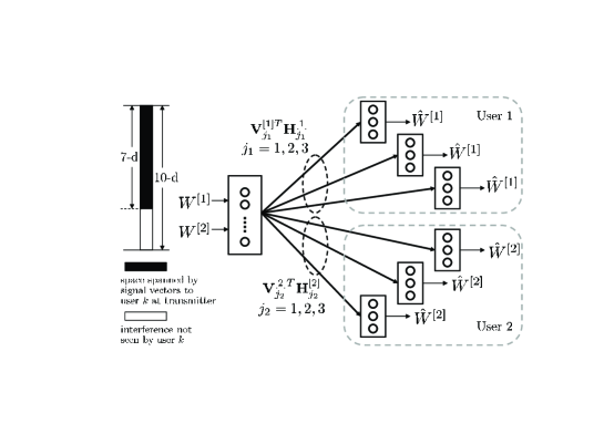
Figure 5: $2$ user MISO compound broadcast channel, $M=2,J_{1}=J_{2}=3$, 5 channel extensions

Consider a complex compound MISO broadcast channel with $K=2$ users, 2 antennas at transmitter, 1 antenna at each receiver, and $J_{1}=J_{2}=J=3$ fading states. It is shown in Theorem 7 of [10] that a total of $\frac{2J}{2J-M+1}=\frac{6}{5}$ DoF can be achieved in this case. This is done by coding over 5 consecutive time slots to achieve 3 DoF for each user. With 5 time slots, the original $1\times 2$ MISO channel ${\bf h}_{j_{k}}^{[k]}$ is converted to a $5\times 10$ MIMO channel ${\bf H}_{j_{k}}^{[k]}$ but the channel has a block diagonal structure, i.e. ${\bf H}_{j_{k}}^{[k]}={\bf h}_{j_{k}}^{[k]}\otimes{\bf I}_{5\times 5}$, where $\otimes$ indicates the Kronecker product operation. For fading state $j_{k}=1,2,3$ of user $k=1,2$, a $5\times 3$ linear combining matrix ${\bf V}_{j_{k}}^{[k]}$ is used whose column vectors are respectively chosen from 3 columns of a $5\times 5$ identity matrix for user 1 and DFT matrix for user 2 such that as seen by the transmitter the space spanned by column vectors of $\left[{\bf H}_{1}^{[k]T}{\bf V}_{1}^{[k]}~{}{\bf H}_{2}^{[k]T}{\bf V}_{2}^{[k]}~{}{\bf H}_{3}^{[k]T}{\bf V}_{3}^{[k]}\right]$ has 7 dimensions (see Figure 5). In other words, from the transmitter’s point of view, the total number of dimensions to be protected for user $k$ is equal to 7. Since the transmitter has access to 10 dimensions, it can send 3 data streams to each user along directions orthogonal to the dimensions occupied by the other user. Thus, each user can get 3 interference free data streams and a total of $\frac{6}{5}$ DoF is achieved per channel use. Note that if ${\bf V}_{j_{k}}^{[k]},j_{k}=1,2,3~{}k=1,2$ are generated randomly, the column space spanned by $\left[{\bf H}_{1}^{[k]T}{\bf V}_{1}^{[k]}~{}{\bf H}_{2}^{[k]T}{\bf V}_{2}^{[k]}~{}{\bf H}_{3}^{[k]T}{\bf V}_{3}^{[k]}\right]$ would have 9 dimensions. Therefore, interference alignment is the key to the achievable scheme of [10].

It turns out, this is not the most efficient interference alignment scheme. The following theorem disproves Conjecture 2 through another counter example.

Theorem 2

For the complex compound MISO BC with $K=2$ users, $M=2$ antennas at the transmitter and $J_{1}=J_{2}=J=3$ generic channel states for each user, the exact number of total DoF = $\frac{4}{3}$, almost surely.

Since $\frac{2J}{2J-M+1}=\frac{6}{5}<\frac{4}{3}$, Conjecture 2 is disproved by Theorem 2. Once again, Theorem 2 indicates that the total number of DoF does not decrease as the number of possible channel states $J$ for each user increases from 2 to 3.

The proof of Theorem 2 is based on asymmetric complex signaling over multiple channel uses and is deferred to Appendix B. Except for the detailed nuances required to deal with the channel structure imposed by channel extensions, the essence of the proof follows from the same interference alignment ideas outlined in the previous section for Theorem 1.

Theorem 1 and 2 present only specific counter examples to disprove Conjectures 1 and 2. In both cases the DoF are shown to remain unchanged as the number of possible states for one or both users is increased by one. From these results it is still not clear what happens as the number of states continues to increase. The problem with extending the results above lies with the limitations of the linear interference alignment approach when channel values are held constant. The difficulty is similar to the problem of characterization of the DoF of the $K$ user interference channel. Linear alignment solutions were shown in that case to achieve the $\frac{K}{2}$ outer bound under time-varying/frequency-selective channel conditions [3]. For the constant channel case, even though asymmetric complex signaling was able to achieve $\frac{6}{5}$ (i.e. greater than one) DoF, it was still away from the $\frac{K}{2}$ outer bound. Interestingly, lattice alignment schemes were needed to show the achievability of $\frac{K}{2}$ DoF almost surely [16, 15]. For the compound MISO BC as well, it turns out that complete DoF characterizations can be found using lattice alignment schemes in the real setting, i.e. where all channel coefficients, signals and noise terms are real variables.

3 Compound MISO Broadcast Channel - Real Setting

We consider the real compound broadcast channel for which the channel input-output relationship is similar to the complex case but with the channel, input signal and noise terms restricted to real values. In the real setting, the total number of degrees of freedom, $d$, is defined as

$$d=\lim_{P\rightarrow\infty}\frac{R^{[1]}+\cdots+R^{[K]}}{\frac{1}{2}{\log P}}$$ (10)

Note that in the previous section, we solved the interference alignment problem for the complex compound BC only by viewing the complex variables as two dimensional real vectors. Therefore it may not be clear why the real setting should be considered separately. The answer lies in the structure of the channel. Translating the complex setting into the real setting, as mentioned before, imposes a special structure on the channel because complex scalar coefficients get replaced with quaternionic matrices. However, in this section we will assume generic real channel coefficients, i.e. the channel coefficients will, almost surely, be algebraically independent over rationals. The connections to the complex setting will be discussed in Section 6.

3.1 Interference Alignment in rational dimensions

It is well known that a multi-dimensional signal space provides multiple independent signalling dimensions. By communicating along linearly independent (beamforming) vectors, different data streams can be separated. Moreover, in a multiuser communication network where interference exists, linear independence between desired signal and interference can be used to separate them as well. The number of DoF is essentially equal to the number of interference free dimensions. Thus, to maximize the achievable DoF, we should minimize the dimension occupied by interference. This is the idea of linear interference alignment, which is exploited to align interference in signal space provided by spatial/time/frequency dimensions [3, 4].

For a network with real constant channel coefficients and single antenna nodes, the notion of signal level as a dimension is very useful. Alignment in this dimension is achieved through multi-level lattice codes, e.g. [19, 20, 16, 18]. Recent work by Etkin and Ordentlich in [16] and by Motahari et. al. [18, 15] shows that interference alignment can be exploited in signal scale dimension based on the notion of rational independence. In this case, different data streams are multiplexed using rationally independent coefficients. In fact, rationally independent coefficients in scalar channels play the same role as linearly independent vectors in vector channels. They serve as distinct directions along which several data streams can be carried simultaneously and can be exploited to separate interference and desired signals as well. In addition, similar to the case in signal space, we can determine the number of DoF by simply counting the number of interference free rational dimensions. Instead of providing 1 DoF per dimension in the signal space, in an $m$ dimensional rational space each dimension can carry $\frac{1}{m}$ degrees of freedom if certain conditions are satisfied. Intuitively, this is because for a 1 dimensional signal space, only 1 DoF is available, and hence each rational dimension can carry $\frac{1}{m}$ DoF.

Next, we summarize the conditions in [18] under which each data stream can achieve $\frac{1}{m}$ DoF in interference networks to multiuser wireless networks where $m$ denotes the maximum number of rational dimensions received among all receivers. As in [18], we denote a set of monomials with variables from a set of algebraically independent numbers over rational numbers as $\mathcal{G}(\mathbf{h})$. In other words, a member of $\mathcal{G}(\mathbf{h})$ is of the form $h_{1}^{\alpha_{1}}h_{2}^{\alpha_{2}}\cdots h_{n}^{\alpha_{n}}$ where $\alpha_{1},\ldots,\alpha_{n}$ are nonnegative integers and $h_{1},\ldots,h_{n}$ are algebraically independent over the rational numbers. Note that all members in $\mathcal{G}(\mathbf{h})$ are rationally independent.

Consider a multiuser wireless network with real channel coefficients where there are $S$ transmitters and $D$ receivers. Each transmitter may have a message for each receiver. For any $\epsilon>0$, transmitter $i,\forall i=1,2,\ldots,S,$ generates $D_{i}$ independent data streams by uniformly picking up integers from interval $(-P^{\frac{1-\epsilon}{2(m+\epsilon)}},P^{\frac{1-\epsilon}{2(m+\epsilon)}})$. Essentially, each data stream carries $\frac{1}{m}$ DoF. Then these data streams are multiplexed by rationally independent numbers $V_{i0},V_{i1},\ldots,V_{i(D_{i}-1)}$ which serve as distinct directions. In order to satisfy the power constraint, the signal is transmitted with a scaling factor $A=\lambda P^{\frac{m-1+2\epsilon}{2(m+\epsilon)}}$ where $\lambda$ is a constant. Now, suppose at receiver $j$, there are $L_{j}$ desired data streams received along directions $V^{\prime}_{j0},V^{\prime}_{j1},\ldots,V^{\prime}_{j(L_{j}-1)}$ and interference data streams are received in a $L^{\prime}_{j}$ dimensional space over rational numbers with a basis $U_{j0},U_{j1},\ldots,U_{j(L^{\prime}_{j}-1)}$. In other words, there are $L^{\prime}_{j}$ effective interference data streams along directions $U_{j0},U_{j1},\ldots,U_{j(L^{\prime}_{j}-1)}$. Each data stream can almost surely achieve a rate $\frac{1}{2m}\log P+o(\log P)$ and hence $\frac{1}{m}$ degrees of freedom where $m$ is the maximum number of rational dimensions received among all receivers, i.e., $m=\max_{j}L_{j}+L^{\prime}_{j}$, if following conditions are satisfied:

1. $V_{i0},V_{i1},\ldots,V_{i(D_{i}-1)}$ are distinct members of $\mathcal{G}(\mathbf{h})$.

2. $V^{\prime}_{j0},V^{\prime}_{j1},\ldots,V^{\prime}_{j(L_{j}-1)}$, $U_{j0},U_{j1},\ldots,U_{j(L^{\prime}_{j}-1)}$ are all distinct.

3. One of $V^{\prime}_{j0},V^{\prime}_{j1},\ldots,V^{\prime}_{j(L_{j}-1)}$, $U_{j0},U_{j1},\ldots,U_{j(L^{\prime}_{j}-1)}$ is 1.

Note that the first condition ensures that $V_{i0},V_{i1},\ldots,V_{i(D_{i}-1)}$ are rationally independent and the second condition ensures that the desired signals and interference are rationally independent so that they can be separated. Along with the first and second condition, the third condition can be used to show that the distance between any two points in the receive constellation grows with $P$ [18]. Thus, at high SNR, the message can be decoded with arbitrary small probability. In addition, as in [18], if none of $V^{\prime}_{j0},V^{\prime}_{j1},\ldots,V^{\prime}_{j(L_{j}-1)}$, $U_{j0},U_{j1},\ldots,U_{j(L^{\prime}_{j}-1)}$ is 1, then $\frac{1}{m+1}$ degrees of freedom can be achieved for each data stream.

We can see that to maximize the achievable DoF, the key is to minimize the dimensions of the space spanned by interference. Note that here the space denotes the set of all linear combinations of rationally independent numbers with rational coefficients. Ideally, we wish to align interference from different users perfectly with each other. For example, if the interference received at one receiver from the $i$th user is along members of $h_{i}\mathbf{V}_{i},\forall i=1,\ldots,N$, we wish to align them as $\textrm{span}(h_{1}\mathbf{V}_{1})=\textrm{span}(h_{2}\mathbf{V}_{2})=\cdots=\textrm{span}(h_{N}\mathbf{V}_{N})$ where $\textrm{span}(A)$ denotes the space spanned by columns of $A$. However, it turns out that such alignment is infeasible in general. In fact, similar problem appears in vector space alignment for interference networks and wireless $X$ networks as well [3, 4]. Fortunately, as shown in [3, 4] alignment is feasible if we allow a negligible fraction of interference terms not aligned perfectly. Due to the similarity of spatial dimensions and rational dimensions, the vector space alignment schemes can be directly translated into alignment schemes in rational dimensions. We present the idea in the following lemma.

Lemma 1

Suppose $T_{1},T_{2},\cdots,T_{N}$ are algebraically independent over the rational numbers. For any $n\in\mathbb{N}$, we can construct a $1\times n^{N}$ vector $\mathbf{V}$ whose entries are rationally independent and a $1\times(n+1)^{N}$ vector $\mathbf{U}$ whose entries are rationally independent as well, such that the following relations are satisfied.

$$\textrm{span}(T_{1}\mathbf{V}) \subset \textrm{span}(\mathbf{U})$$

$$\textrm{span}(T_{2}\mathbf{V}) \subset \textrm{span}(\mathbf{U})$$

$$\vdots$$

$$\textrm{span}(T_{N}\mathbf{V}) \subset \textrm{span}(\mathbf{U})$$

Proof: Let us construct two sets $V$ and $U$ with cardinality $n^{N}$ and $(n+1)^{N}$, respectively, as follows:

$$V = \big{\{}\prod_{i=1,\ldots,N}T_{i}^{\alpha_{i}}:(\alpha_{1},\ldots,\alpha_{N})\in\{1,2\ldots,n\}^{N}\big{\}}$$ (11)

$$U = \big{\{}\prod_{i=1,\ldots,N}T_{i}^{\alpha_{i}}:(\alpha_{1},\ldots,\alpha_{N})\in\{1,2\ldots,n+1\}^{N}\big{\}}$$ (12)

Since elements of $V$ are distinct monomials, they are rationally independent. Similarly, elements of $U$ are rationally independent. Let entries of $\mathbf{V}$ and $\mathbf{U}$ be the elements of $V$ and $U$, respectively. It can be easily seen that such construction satisfies all conditions stated above.  

Note that the span of a vector here represents the set of all real numbers that can be represented as linear combinations of the elements of the vector with rational coefficients.

It is important to note that the construction of $V$ and $U$ requires the commutative property of multiplication of numbers $T_{i}$. For vector space alignment schemes in interference networks and wireless $X$ networks [3, 4], $T_{i}$ are diagonal matrices which satisfy commutative property of multiplication as well. Notice that as $n\rightarrow\infty$, $\frac{|V|}{|U|}\approx 1$. This implies that these two sets are asymptotically perfectly aligned.

3.2 Degrees of Freedom of Compound Broadcast Channel

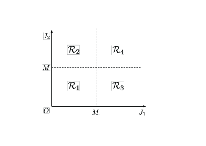
Figure 6: $4$ regions for $2$ User Compound Broadcast Channel

In this section, we first consider the 2 user compound broadcast channel with $J_{1}$ and $J_{2}$ states at each user, respectively. First, according to the relationship between $J_{i}$ and $M$, we partition the $J_{1}$ and $J_{2}$ plane into four distinct regions as illustrated in Figure 6. It can be seen that in the first region $\mathcal{R}_{1}$ where $J_{1}<M$ and $J_{2}<M$, each user can achieve 1 degrees of freedom [10]. This can be done by transmitting a data stream along a beamforming vector orthogonal to channels of the other user. Thus, in this region, each user achieves the same degrees of freedom as non-compound broadcast channel. In other words, no degrees of freedom is lost due to multiple states at each user.

Next we consider regions $\mathcal{R}_{2}$ and $\mathcal{R}_{3}$ in which the number of states for at least one user is no less than $M$ while the other user has less than $M$ states. We establish the total number of degrees of freedom for these two regions in the following theorem.

Theorem 3

For the compound real broadcast channel with $M$ antennas at the transmitter, $2$ single antenna users with $J_{1}<M$ and $J_{2}\geq M$ or $J_{2}<M$ and $J_{1}\geq M$, the exact number of total degrees of freedom is $1+\frac{M-1}{M}$ almost surely.

Proof: The outer bound follows from [10]. Due to symmetry, let us consider the case when $J_{1}<M$ and $J_{2}\geq M$. We will show user 1 can achieve 1 DoF while user 2 achieves $\frac{M-1}{M}$ DoF. First, note that when $J_{2}=M$, this can be achieved using zero-forcing at the transmitter [10]. Now consider $J_{2}>M$. For simplicity, let us consider the case when $M=2$, $J_{1}=1$ and $J_{2}=3$. The proof for the general case is presented in the Appendix. Thus, we need to show that user 1 and 2 can achieve 1 and $\frac{1}{2}$ degrees of freedom, respectively. Note that the linear alignment solution presented previously for the complex channel does not apply here, with generic real channel coefficients.

Message $W^{[1]}$ intended for user 1 is split into $2$ sub-messages denoted as $W^{[1]}_{1}$ and $W^{[1]}_{2}$. $W^{[1]}_{1}$ is encoded into $n^{6}$ data streams denoted as $X^{[1]}_{1k},~{}k=1,\ldots,n^{6}$. $W^{[1]}_{2}$ is encoded into $n^{6}$ data streams denoted as $X^{[1]}_{2k},~{}k=1,\ldots,n^{6}$. Message for user 2 denoted as $W^{[2]}$ is encoded into $n^{6}$ independent data streams denoted as $X^{[2]}_{k},~{}k=1,\ldots,n^{6}$. For any $\epsilon>0$, let $\mathcal{C}=\{x:x\in\mathbb{Z}\cap[-P^{\frac{1-\epsilon}{2(m_{n}+\epsilon)}},P^{\frac{1-\epsilon}{2(m_{n}+\epsilon)}}]\}$ where $m_{n}=1+(n+1)^{6}+n^{6}$. In other words, $\mathcal{C}$ denotes a set of all integers in the interval $[-P^{\frac{1-\epsilon}{2(m_{n}+\epsilon)}},P^{\frac{1-\epsilon}{2(m_{n}+\epsilon)}}]$. Each symbol in the data stream is obtained by uniformly i.i.d. sampling $\mathcal{C}$. Essentially, each data stream carries $\frac{1}{m_{n}}$ degrees of freedom.

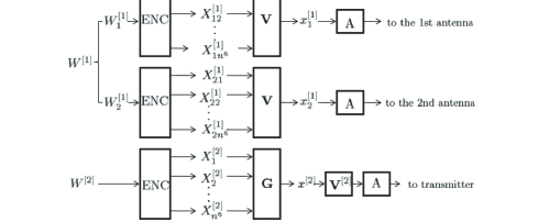
Figure 7: Encoding at transmitter 1 and 2 for 2 user compound broadcast channel

A data stream $x^{[1]}_{i},\forall i=1,2$ is obtained by multiplexing data streams $X^{[1]}_{ik},\forall k=1,\ldots,n^{6}$ using a $1\times n^{6}$ vector $\mathbf{V}$, i.e, $x^{[1]}_{i}=\mathbf{V}\mathbf{X}^{[1]}_{i}$, where $\mathbf{V}=[V_{1},\ldots,V_{n^{6}}]$ and $\mathbf{X}^{[1]}_{i}=[X^{[1]}_{i1},\ldots,X^{[1]}_{in^{6}}]^{T}$. Note that all elements of $\mathbf{V}$ are functions of channel coefficients which will be designed to align interference. A data stream $x^{[2]}$ is obtained by multiplexing $X^{[2]}_{k},~{}k=1,\cdots,n^{6}$ using a $1\times n^{6}$ vector $\mathbf{G}$, i.e, $x^{[2]}=\mathbf{G}\mathbf{X}^{[2]}$, where $\mathbf{X}^{[2]}=[X^{[2]}_{1},\ldots,X^{[2]}_{n^{6}}]^{T}$. Let $\mathbf{G}=[G_{0}~{}G^{2}_{0}~{}\cdots~{}G^{n^{6}}_{0}]$ where $G_{0}$ is a randomly generated real number which is algebraically independent with all channel coefficients over rationals almost surely. After scaling with a factor $A$, $x^{[2]}$ is transmitted with a beamforming vector $\mathbf{V}^{[2]}$ and $x^{[1]}_{i}$ is transmitted from the $i$th antenna as illustrated in Figure 7. Thus, the transmitted signal is

$$\mathbf{x}=A(\mathbf{V}^{[2]}x^{[2]}+\mathbf{X}^{[1]})$$ (13)

where $\mathbf{X}^{[1]}=[x^{[1]}_{1}~{}x^{[1]}_{2}]^{T}$ and $\mathbf{V}^{[2]}$ with unit norm is orthogonal to the channel of user 1. Thus, no interference is created at user 1. $A$ is a scalar which is chosen such that the power constraint is satisfied, i.e.,

$$E[\|\mathbf{x}\|^{2}] = E[A(\mathbf{V}^{[2]}x^{[2]}+\mathbf{X}^{[1]})^{T}A(\mathbf{V}^{[2]}x^{[2]}+\mathbf{X}^{[1]})]$$ (14)

$$= A^{2}\big{(}E[(x^{[2]})^{2}]+E[(x^{[1]}_{1})^{2}]+E[(x^{[1]}_{2})^{2}]\big{)}$$

$$\leq A^{2}\underbrace{(\|\mathbf{G}\|^{2}+2\|\mathbf{V}\|^{2})}_{\lambda^{2}}P^{\frac{1-\epsilon}{m_{n}+\epsilon}}$$

$$\leq P$$

$$\Rightarrow A = \frac{1}{\lambda}P^{\frac{m_{n}+2\epsilon-1}{2(m_{n}+\epsilon)}}$$ (15)

Let us first consider user 2. The received signal at receiver 2 under state $j_{2}$ is given by

$$y^{[2]}_{j_{2}} = A(\mathbf{h}^{[2]}_{j_{2}}(\mathbf{V}^{[2]}x^{[2]}+\mathbf{X}^{[1]}))+z^{[2]}_{j_{2}}$$ (16)

$$= A(\underbrace{\mathbf{h}^{[2]}_{j_{2}}\mathbf{V}^{[2]}}_{h^{[2]^{\prime}}_{j_{2}}}x^{[2]}+\mathbf{h}^{[2]}_{j_{2}}\mathbf{X}^{[1]})+z^{[2]}_{j_{2}}$$

$$= A(h^{[2]^{\prime}}_{j_{2}}\mathbf{G}\mathbf{X}^{[2]}+h^{[2]}_{j_{2}1}\mathbf{V}\mathbf{X}^{[1]}_{1}+h^{[2]}_{j_{2}2}\mathbf{V}\mathbf{X}^{[1]}_{2})+z^{[2]}_{j_{2}},~{}~{}\forall j_{2}=1,2,3$$

where $\mathbf{h}^{[2]}_{j_{2}}=[h^{[2]}_{j_{2}1}~{}h^{[2]}_{j_{2}2}]$. In order for desired signal $\mathbf{X}^{[2]}$ to get $n^{6}$ interference free dimensions in a total of $1+(n+1)^{6}+n^{6}$ dimensional space, we align all interference into a $(n+1)^{6}$ dimensional subspace which is spanned by the members of a $1\times(n+1)^{6}$ vector $\mathbf{U}$:

$$\textrm{span}(h^{[2]}_{j_{2}i}\mathbf{V}) \subset \textrm{span}(\mathbf{U}),~{}~{}j_{2}=1,2,3~{}~{}i=1,2$$ (17)

From Lemma 1, we construct $\mathbf{V}$ and $\mathbf{U}$ with rationally independent members to satisfy above equations. Since $\mathbf{G}$ is generated independently with $\mathbf{\mathbf{U}}$, members of $h^{[2]^{\prime}}_{j_{2}}\mathbf{G}$ and $\mathbf{U}$ are all distinct and none of them is equal to 1. Thus, user 2 can achieve $\frac{n^{6}}{1+n^{6}+(n+1)^{6}}$ degrees of freedom regardless of the realization of the channel almost surely. As $n\rightarrow\infty$, $\frac{1}{2}$ degrees of freedom can be achieved.

Now consider user 1. Since there is no interference at user 1, all data streams are received interference free and along elements $h^{[1]}_{1}\mathbf{V}$ and $h^{[1]}_{2}\mathbf{V}$ where $h^{[1]}_{i}$ is the channel coefficient from the $i$th antenna to user 1. It can be easily seen that members of $h^{[1]}_{1}\mathbf{V}$ and $h^{[1]}_{2}\mathbf{V}$ are all distinct since $\mathbf{V}$ is independent of $h^{[1]}_{i}$. In addition, none of them is 1. Notice that there are a total of $2n^{6}$ data streams. Since each stream carries $\frac{1}{1+(n+1)^{6}+n^{6}}$ degrees of freedom, user 1 achieves a total of $\frac{2n^{6}}{1+(n+1)^{6}+n^{6}}$ DoF almost surely. As $n\rightarrow\infty$, 1 DoF can be achieved.  

As in the complex setting, this is a surprising result. Intuitively, the DoF will decrease as the number of states associated with the user increases. However, Theorem 3 shows that if one user’s states are less than $M$ and regardless of the number of states associated with the other user, $1+\frac{M-1}{M}$ DoF can be achieved. Thus, in regions $\mathcal{R}_{2}$ and $\mathcal{R}_{3}$, there is only a fraction of $\frac{1}{M}$ DoF lost due to multiple states at users.

Next we establish the degrees of freedom for $\mathcal{R}_{4}$ by solving a general case, i.e., a $N\geq 2$ users compound broadcast channel where each user has no less than $M$ states. The result is presented in the following theorem.

Theorem 4

For the real compound broadcast channel with $M$ antennas at the transmitter, $N$ single antenna users with $J_{i}\geq M,i=1,\ldots,N$ states at user $i$, the total number of degrees of freedom is $\frac{MN}{M-N+1}$ almost surely.

Proof: The achievable scheme is based on $M\times N$ compound $X$ channel discussed later in Theorem 5. Since the compound $X$ channel is a restricted form of the MISO BC (the transmit antennas are separated in the $X$ channel), achievable degrees of freedom for the $X$ channel are also achievable for the BC.

For the outer bound, we consider the case where $J_{1}=1$ and $J_{i}=M,i=2,\cdots,N$, since adding more states for each user results in more constraints and hence cannot increase the rates. The bound is obtained for a degraded broadcast channel by providing receiver $1$ to $N-1$ with all received signals. Let $\mathbf{Y}^{[i]}=[y^{[i]}_{1}\cdots y^{[i]}_{J_{i}}]$ denote the received signals for all realizations of user $i$. For an auxiliary random variable $U$, $U-\mathbf{x}-(y^{[1]},\mathbf{Y}^{[2]},\cdots,\mathbf{Y}^{[N]})-y^{[N]}_{i}$ forms a Markov chain. Thus, we have

$$R^{[1]}+R^{[2]}+\cdots+R^{[N-1]}$$ (18)

$$\leq I(\mathbf{x};y^{[1]},\mathbf{Y}^{[2]},\cdots,\mathbf{Y}^{[N]}|U)$$

$$= I(\mathbf{x};\mathbf{Y}^{[N]}|U)+I(\mathbf{x};y^{[1]},\mathbf{Y}^{[2]},\cdots,\mathbf{Y}^{[N-1]}|U,\mathbf{Y}^{[N]})$$

$$= I(\mathbf{x};\mathbf{Y}^{[N]}|U)+o(\log P)$$

$$= \sum_{i=1}^{M}I(\mathbf{x};y^{[N]}_{i}|y^{[N]}_{1},\ldots,y^{[N]}_{i-1},U)+o(\log P)$$

$$= \sum_{i=1}^{M}\big{(}h(y^{[N]}_{i}|y^{[N]}_{1},\ldots,y^{[N]}_{i-1},U)-h(y^{[N]}_{i}|y^{[N]}_{1},\ldots,y^{[N]}_{i-1},U,\mathbf{x})\big{)}+o(\log P)$$

$$\leq \sum_{i=1}^{M}\big{(}h(y^{[N]}_{i}|U)-h(y^{[N]}_{i}|U,\mathbf{x})\big{)}+o(\log P)$$

$$= \sum_{i=1}^{M}I(\mathbf{x};y^{[N]}_{i}|U)+o(\log P)$$

On the other hand, $\forall i=1,\ldots,M$,

$$R_{N} \leq I(U;y^{[N]}_{i})$$ (19)

Adding up all these bounds, we have

$$MR_{N}\leq\sum_{i=1}^{M}I(U;y^{[N]}_{i})$$ (20)

Now adding (18) and (20), we have

$$R^{[1]}+\cdots+R^{[N-1]}+MR^{[N]} \leq \sum_{i=1}^{M}(I(U;y^{[N]}_{i})+I(\mathbf{x};y^{[N]}_{i}|U))+o(\log P)$$ (21)

$$= \sum_{i=1}^{M}I(\mathbf{x};y^{[N]}_{i})+o(\log P)$$

$$\leq \frac{M}{2}\log P+o(\log P)$$

By symmetry, $\forall i=1,\ldots,N-1$, we have

$$R^{[1]}+\cdots+R^{[i-1]}+MR^{[i]}+R^{[i+1]}+\cdots+R^{[N]}\leq\frac{M}{2}\log P+o(\log P)$$ (22)

Adding up all such bounds, we have

$$(M+N-1)(R^{[1]}+\cdots+R^{[N]}) \leq \frac{MN}{2}\log P+o(\log P)$$

$$\Rightarrow R^{[1]}+\cdots+R^{[N]} \leq \frac{MN}{2(M+N-1)}\log P+o(\log P)$$ (23)

Therefore,

$$d^{[1]}+\cdots+d^{[N]}=\lim_{P\rightarrow\infty}\frac{R^{[1]}+\cdots+R^{[N]}}{\frac{1}{2}\log P}\leq\frac{MN}{M+N-1}$$ (24)

 

Thus we have shown that the DoF of the (real) finite state compound MISO BC do not collapse to 1 as the channel uncertainty (number of possible states) increases. What is lost is only the DoF benefits of joint processing at the transmit antennas, without which the MISO BC reduces to an $X$ network. Note that for large $M$ this loss also disappears. In other words, for large $M$, the MISO BC with $N$ users and arbitrary number of states at each user, can achieve $\frac{MN}{M+N-1}\approx N$ DoF which is the maximum DoF possible with perfect CSIT.

4 Compound $X$ Channel

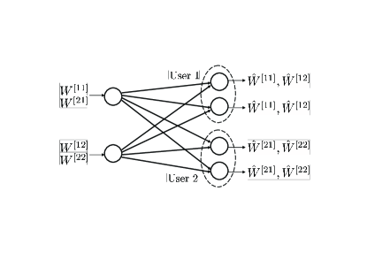
Figure 8: $2$ User Compound $X$ Channel with $J_{1}=J_{2}=2$

The $M\times N$ wireless compound $X$ channel consists of $M$ transmitters and $N$ receivers. Transmitter $i,\forall i=1,\ldots,M$ sends an independent message $W^{[ji]}$ with rate $R^{[ji]}$ to receiver $j,\forall j=1,\ldots,N$. Thus, there are a total of $MN$ messages in the network. Let us denote the channel vector associated with receiver $j,~{}\forall j\in\{1,\ldots,N\}$ as a vector $(h^{[j1]},\cdots,h^{[jM]})$ which is drawn from a finite set $\mathcal{J}_{j}$ with cardinality $J_{j}$. In addition, we assume the channel states are drawn from a continuous distribution and hence algebraically independent over rational numbers almost surely. Once the channel is drawn, it remains fixed during the entire transmission. While the transmitters are unaware of the specific channel state realization, the receivers are assumed to have perfect channel knowledge. We say the rate tuple $(R^{[11]},\ldots,R^{[NM]})$ is achievable if all messages can be decoded with arbitrarily small error probability regardless of the channel realizations. In this paper, we mainly consider the real compound $X$ channel. The received signal at receiver $j$ under state $k_{j}$ is given by

$$y^{[j]}_{k_{j}}=\sum_{i=1}^{M}h^{[ji]}_{k_{j}}x^{[i]}+z^{[j]}_{k_{j}}~{}~{}k_{j}=1,\ldots,J_{j},~{}j=1,\ldots,N$$ (25)

where $h^{[ji]}_{k_{j}}$ and $x^{[i]}$ represent the channel coefficient and transmitted signal, respectively. Transmitter $i$ satisfies the power constraint $E(x_{i}^{2})\leq P$. $z^{[j]}_{k_{j}}$ is the additive white Gaussian noise (AWGN) with zero mean and unit variance. The total number of degrees of freedom, $d$, is defined as

$$d=\lim_{P\rightarrow\infty}\frac{R^{[11]}+\cdots+R^{[NM]}}{\frac{1}{2}\log P}$$ (26)

A two user compound $X$ channel with 2 states at each user is shown in Figure 8.

4.1 Degrees of Freedom of Compound $X$ Network

We establish the total number of DoF for real compound $X$ network in the following theorem.

Theorem 5

For the real compound $M\times N$ $X$ network with $J_{j}$ states associated at the $j$th receiver, the total number of degrees of freedom is $\frac{MN}{M+N-1}$ almost surely.

Proof: For the non-compound $X$ network, [4] shows that the total degrees of freedom cannot be more than $\frac{MN}{M+N-1}$. Since compound $X$ network has more decoding constraints, the outer bound for non-compound $X$ network is also an outer bound for the compound $X$ network. Next, we provide an outline of achievable scheme for $2\times 2$ user $X$ network with 2 states at each user. The detailed proof for general case is provided in the Appendix.

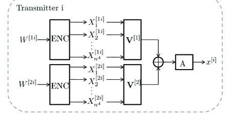
Figure 9: Encoding at transmitter $i$

The message from transmitter $i(i=1,2)$, to receiver $j(j=1,2)$ denoted as $W^{[ji]}$, is encoded into $n^{4}$ independent data streams. Let $X^{[ji]}_{k}$ denote the symbol of $k$th data streams from transmitter $i$ to receiver $j$. For any $\epsilon>0$, let $\mathcal{C}=\{x:x\in\mathbb{Z}\cap[-P^{\frac{1-\epsilon}{2(m_{n}+\epsilon)}},P^{\frac{1-\epsilon}{2(m_{n}+\epsilon)}}]\}$ where $m_{n}=1+(n+1)^{4}+2n^{4}$. Each symbol in the data stream is obtained by uniformly i.i.d. sampling $\mathcal{C}$. Essentially, each symbol carries $\frac{1}{m_{n}}$ degrees of freedom.

At transmitter $i,\forall i=1,2$, the transmitted signal for user $j$ is obtained by multiplexing different data streams using a vector $\mathbf{V}^{[j]}$. After scaling with a factor $A$, the transmitted signal is

$$x^{[i]} = A(\mathbf{V}^{[1]}\mathbf{X}^{[1i]}+\mathbf{V}^{[2]}\mathbf{X}^{[2i]})~{}~{}i=1,2$$ (27)

where $\mathbf{X}^{[ji]}=[X^{[ji]}_{1}X^{[ji]}_{2}\cdots X^{[ji]}_{n^{4}}]^{T}$ and $\mathbf{V}^{[j]}=[V^{[j]}_{1}~{}V^{[j]}_{2}\cdots V^{[j]}_{n^{4}}]~{}\forall j=1,2$. The encoding at the transmitter is illustrated in Figure 9. $A$ is a scalar which is designed such that the power constraints are satisfied, i.e.,

$$E((x^{[i]})^{2})\leq P~{}~{}\forall i=1,2$$ (28)

$$E((x^{[i]})^{2})\leq A^{2}P^{\frac{1-\epsilon}{m_{n}+\epsilon}}\sum_{j=1}^{2}\|\mathbf{V}^{[j]}\|^{2}\leq P$$ (29)

Let $\lambda^{2}=\sum_{j=1}^{2}\|\mathbf{V}^{[j]}\|^{2}$ which is a constant, then

$$A^{2}P^{\frac{1-\epsilon}{m_{n}+\epsilon}}\lambda^{2} \leq P$$ (30)

$$\Rightarrow A = \frac{1}{\lambda}P^{\frac{m_{n}-1+2\epsilon}{2(m_{n}+\epsilon)}}$$ (31)

The received signal for the first state at receiver 1 is given by:

$$y^{[1]}_{1} = \sum_{i=1}^{2}h^{[1i]}_{1}x_{i}+z^{[1]}_{1}$$

$$= A(\underbrace{h_{1}^{[11]}\mathbf{V}^{[1]}\mathbf{X}^{[11]}+h^{[12]}_{1}\mathbf{V}^{[1]}\mathbf{X}^{[12]}}_{\textrm{desired signal}}+\underbrace{h_{1}^{[11]}\mathbf{V}^{[2]}\mathbf{X}^{[21]}+h_{1}^{[12]}\mathbf{V}^{[2]}\mathbf{X}^{[22]}}_{\textrm{interference}})+z^{[1]}_{1}$$

In order to get $2n^{4}$ interference free dimensions for desired signal in a total of $1+2n^{4}+(n+1)^{4}$ dimensional space, we align all interference into a $(n+1)^{4}$ dimensional subspace spanned by members of $\mathbf{U}^{[2]}$:

$$\textrm{span}(h^{[11]}_{1}\mathbf{V}^{[2]}) \subset \textrm{span}(\mathbf{U}^{[2]})$$ (32)

$$\textrm{span}(h^{[12]}_{1}\mathbf{V}^{[2]}) \subset \textrm{span}(\mathbf{U}^{[2]})$$ (33)

Similarly, for the second state at receiver 1, we have following alignment conditions:

$$\textrm{span}(h^{[11]}_{2}\mathbf{V}^{[2]}) \subset \textrm{span}(\mathbf{U}^{[2]})$$ (34)

$$\textrm{span}(h^{[12]}_{2}\mathbf{V}^{[2]}) \subset \textrm{span}(\mathbf{U}^{[2]})$$ (35)

By symmetry, the alignment conditions for user 2 are

$$\textrm{span}(h^{[22]}_{i}\mathbf{V}^{[1]}) \subset \textrm{span}(\mathbf{U}^{[1]})$$ (36)

$$\textrm{span}(h^{[21]}_{i}\mathbf{V}^{[1]}) \subset \textrm{span}(\mathbf{U}^{[1]})~{}~{}i=1,2$$ (37)

From Lemma 1, we can construct $\mathbf{V}^{[1]}$, $\mathbf{V}^{[2]}$, $\mathbf{U}^{[1]}$ and $\mathbf{U}^{[2]}$ to satisfy those equations. As a result, all interference is received along members of $\mathbf{U}^{[1]}$ and $\mathbf{U}^{[2]}$ at user 2 and 1, respectively. It can be seen that members of $\mathbf{V}^{[1]}$ and $\mathbf{V}^{[2]}$ are distinct and rationally independent. Notice that members of $\mathbf{V}^{[1]}$ and $\mathbf{U}^{[1]}$ depend on $h^{[22]}_{i}$ and $h^{[21]}_{i}$, $\forall i=1,2$ while members of $\mathbf{V}^{[2]}$ and $\mathbf{U}^{[2]}$ depend on $h^{[12]}_{i}$ and $h^{[11]}_{i}$. Thus, all the desired data streams are received along distinct directions from the interference and none of them is 1. Thus, each message can achieve $\frac{n^{4}}{1+(n+1)^{4}+2n^{4}}$ degrees of freedom almost surely regardless of channel realizations. As $n\rightarrow\infty$, each message achieves $\frac{1}{3}$ degrees of freedom for a total of $\frac{4}{3}$ degrees of freedom.  

Remark: Theorem 5 also establishes the total degrees of freedom for the real $M\times N$ wireless $X$ network with constant channel coefficients are $\frac{MN}{M+N-1}$ almost surely. Since this is a special case of compound $X$ network when each user has only one state. In addition, this indicates that the finite state compound $X$ channel does not lose any DoF compared to the non-compound setting.

5 Compound Interference Channel

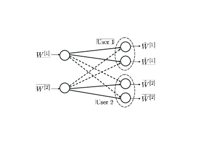
Figure 10: $2$ User Compound Interference Channel with $J_{1}=J_{2}=2$

A $K$ user compound interference channel consists of $K$ transmitter and receiver pairs. Each transmitter sends an independent message $W^{[j]},\forall j=1,\ldots,K$ with rate $R^{[j]}$ to its receiver. Channels associated with receiver $j$ are denoted as the vector $(h^{[j1]},\cdots,h^{[jM]})$ which comes from a finite set $\mathcal{J}_{j}$ with cardinality $J_{j}$. In addition, we assume the channel states are drawn from a continuous distribution and hence algebraically independent over rational numbers almost surely. Once the channel is drawn, it remains fixed during the entire transmission. While the transmitters are unaware of the specific channel state realization, the receivers are assumed to have perfect channel knowledge. In this section, we consider the real compound interference channel. The received signal at user $j$ under state $k_{j}$ is given by

$$y^{[j]}_{k_{j}}=\sum_{i=1}^{K}h^{[ji]}_{k_{j}}x^{[i]}+z^{[j]}_{k_{j}}~{}~{}~{}k_{j}=1,\ldots,J_{j},~{}\forall j=1,\ldots,K$$ (38)

where $y^{[j]}_{k_{j}}$, $h^{[ji]}_{k_{j}}$ and $x^{[i]}$ represent the received signal, channel coefficient and transmitted signal, respectively. Transmitters satisfy the power constraint $E(x_{i}^{2})\leq P$. $z^{[j]}_{k_{j}}$ is AWGN with zero mean and unit variance. We say a rate tuple $(R^{[1]},\ldots,R^{[K]})$ is achievable if each receiver can decode its message with arbitrarily small error probability regardless of what state is realized. The total number of degrees of freedom, $d$, is defined as

$$d=\lim_{P\rightarrow\infty}\frac{R^{[1]}+\cdots+R^{[K]}}{\frac{1}{2}\log P}$$ (39)

A two user compound interference channel with 2 states at each user is shown in Figure 10.

5.1 Degrees of Freedom of Compound Interference Channel

Similar to compound $X$ channel, $K$ user interference networks do not lose DoF in the finite state compound channel setting. We present the result in the following theorem.

Theorem 6

The degrees of freedom for $K$ user real compound interference channel with finite states at each user are $\frac{K}{2}$ almost surely.

Proof: The proof is provided in the Appendix.  

Remark: Note that if we view different states associated at each receiver as different users which require distinct messages from the corresponding transmitter, it is equivalent to an interference broadcast channel which models the downlink of cellular network. Specifically, consider a cellular network with $M$ cells in each of which there are $K$ users. Then using similar interference alignment schemes used for compound $X$ channel, a total of $\frac{MK}{K+1}$ DoF can be achieved.

6 Discussion on DoF of Complex Compound Wireless Networks

In Section 3, 4 and 5, we establish the total DoF for different real compound wireless networks. A natural question is whether the same results can be obtained for their complex counterparts. The key to answer this question is to determine if the interference alignment schemes used for the real compound interference networks can be adopted in networks with complex channel coefficients. Since the alignment schemes are designed for real channel coefficients, we first write the complex channel as an equivalent channel with real channel coefficients. Consider a point to point complex channel with a complex channel coefficient $h$ and a complex noise term $z$. Then the channel can be written as

$$\left[\begin{array}[]{c}y_{R}\\ y_{I}\end{array}\right]=\left[\begin{array}[]{cc}h_{R}&-h_{I}\\ h_{I}&h_{R}\end{array}\right]\left[\begin{array}[]{c}x_{R}\\ x_{I}\end{array}\right]+\left[\begin{array}[]{c}z_{R}\\ z_{I}\end{array}\right]$$ (48)

where subscripts $R$ and $I$ denote the real and imaginary part of the complex number, respectively. To study the feasibility of the interference alignment schemes of real wireless networks on their complex counterparts, let us first consider the non-compound interference network. In fact, in [18], it is pointed out that for the $K$ user complex interference channel, every user is still able to achieve 1/2 DoF. This can be done by viewing real and imaginary dimensions as two independent users. As a result, a user with complex channel coefficients is converted to a two user real interference channel where the channel input-output relation is given by (48). Thus, instead of a $K$ user complex interference channel, we obtain a $2K$ user real interference channel with some dependence among channel coefficients in the network. Now using the interference alignment scheme on the real interference network, all interference can be aligned at each receiver. Note that all beamforming directions are monomials with variables of all distinct cross links. Since the direct links are distinct with all cross links, the directions of desired signal are distinct of all interference after scaling with the direct channel, and thus the desired signal is rationally independent with all interference. Thus, a total of $K$ real DoF, and hence $K/2$ complex DoF can be achieved. Similarly, the compound complex interference channel also has $K/2$ DoF almost surely.

However, it is difficult to make the same case for the complex compound $X$ channel using a similar approach as in the compound interference channel. It turns out the desired signals overlap with each other. Intuitively, this is because desired links are the same as some interference links. Thus, although we can align signals at receivers where they are not desired, they are aligned at the desired receivers as well. To avoid the dependence among channel coefficients, at the cost of nearly half the DoF, we can restrict the transmitters to send only real signals. For example, for an $M\times 2$ complex compound $X$ channel where the number of states associated with each user is greater than $M$, we can obtain an $M\times 4$ user real compound $X$ channel with all channel coefficients independent with each other. From Theorem 5, $\frac{4M}{M+3}$ real DoF and hence $\frac{2M}{M+3}$ complex DoF can be achieved. Notice that when $M>3$, more than 1 DoF can be achieved. Thus, even for the 2 user complex MISO broadcast channel, more than 1 DoF can be achieved regardless of the number of states as long as the number of antennas at the transmitter is greater than 3.

7 Conclusion

This work was motivated by the need to resolve the remarkable contrast between optimistic results that advocate structured codes based on the high DoF that can be achieved with perfect channel knowledge, and pessimistic conjectures that claim that without perfect channel knowledge the DoF collapse to unity. The strongest pessimistic conjectures were made by Weingarten et. al. in the finite state compound channel setting for the MISO BC. In this work we settle these conjectures in the negative, thereby showing that in the finite state compound channel setting, the DoF results based on structured codes are robust to channel uncertainty at the transmitters.

In retrospect, it is perhaps not too surprising that the finite state compound channel setting does not lose DoF. For example, consider the $K$ user interference channel. Within this channel, consider the signals sent by transmitter 1 and 2. In order to achieve the full $K/2$ DoF, it is clear that these signals must align at receivers $3,4,\cdots,K$. Clearly, as $K$ increases, i.e., more and more receivers are added, bringing new channels into the picture, the signals from transmitter 1 and 2 must be aligned at these new receivers while still maintaining alignment at the previously existing receivers. While it may be surprising at first to find out that this can be done, it has already been shown in [3]. The compound network setting offers a very similar challenge. Whatever alignments are needed, must be achieved for not just one state but for an arbitrary (but finite) number of states. In the $K$ user interference channel example above, if we think of the channels to receivers $3,4,\cdots,K$ as multiple states for the same user, it is clear that the alignment is robust to the number of states.

The key to the robustness of DoF in the finite state compound setting is the same as the key to the $K/2$ DoF of the $K$ user interference channel – unbounded bandwidth expansion, or equivalently unlimited resolution in time, frequency, space, or signal level dimensions. As the alignment problem becomes more and more challenging, whether by increasing the number of states in the compound setting or by increasing the number of users in the $K$ user interference channel, greater and greater bandwidth (equivalently, resolution) is needed to achieve partial alignment. In the time-varying/frequency-selective $K$ user interference channel the bandwidth expansion refers to the need to code over increasingly larger number of symbols. Thinking of these symbols as frequency slots, we call this a bandwidth expansion. Similar bandwidth expansion (equivalent to the unbounded resolution of propagation delays) is observed in the line of sight alignment schemes found in [21, 22]. Interestingly, when we think of signal level as a signaling dimension, the unbounded bandwidth expansion or unlimited resolution essentially corresponds to the infinite precision knowledge of the channel coefficients. With this infinite precision, we have an infinite number of signaling level dimensions along which interference can be aligned regardless of the number of states. Note that the rational/irrational scaled lattice alignment schemes follow a complete translation of the Cadambe-Jafar alignment scheme [3] from the time-varying/frequency-selective channel model to the real constant channel model. Once the role of rational/irrational scaled lattice alignments is understood in this context, it is not surprising that finite state compound networks retain their ability to align signals and thus do not lose their DoF entirely.

While the DoF are not entirely lost in the finite state compound setting, it is intriguing that the benefits of transmitter cooperation are lost. In other words, the MIMO benefits of vector space alignment are lost. This observation may indicate the distinct character of alignment schemes over vector spaces and signal levels. It is notable that inspite of a variety of results on these different alignment approaches, it has not been possible so far to unify them into a common framework to understand their collective synergies and individual limitations.

Another intriguing question that remains open is the implication of real versus complex models. In all well-studied networks so far, this issue has been of no real consequence. For interference alignment problems this issue does become important as it affects the structure of the channel. However, it is not clear if this is an avoidable nuisance or if there is a fundamental distinction between the two settings.

Finally, in the current line of work, the most important issue that remains unresolved is the robustness of DoF characterizations to compound networks with infinite states or a continuum of states. In this regard, the conjecture of Lapidoth et. al. [9] is most relevant, as is the recent work on the DoF of the two user MIMO interference channel [2]. The overarching observation is that the best outer bounds known so far are not able to distinguish between channel uncertainty at the transmitters over a finite set of states or over a continuum of states. To prove the pessimistic hypothesis, if indeed the DoF collapse to unity with channel uncertainty over a continuous (non-zero measure) channel space, then better outer bounds are needed that can distinguish this setting from the finite state compound setting. On the other hand, to prove the optimistic hypothesis, that the DoF are indeed resilient to channel uncertainty over a continuum, then a much finer understanding of statistical interference alignment is needed. In either case, settling this issue will have a profound impact on our understanding of both the capacity limits of wireless networks as well as the robustness of these limits.

Appendix A Proof of Theorem 1

Proof: The converse is shown in [10]. The achievable scheme is interference alignment with asymmetric signaling.

Consider the received signal at user $k$ under state $j_{k}$ in a single time slot.

$$y_{j_{k}}^{[k]}={\bf h}_{j_{k}}^{[k]}{\bf x}+z_{j_{k}}^{[k]}$$ (49)

By viewing complex variables as two dimensional vectors, the received signal can be written as

$$\underbrace{\left[\begin{array}[]{c}\mbox{Re}\{y_{j_{k}}^{[k]}\}\\ \mbox{Im}\{y_{j_{k}}^{[k]}\}\end{array}\right]}_{{\bf y}_{j_{k}}^{[k]}:2\times 1}=\underbrace{\left[\!\!\begin{array}[]{rrrr}\mbox{Re}\{h_{j_{k}1}^{[k]}\}\!\!&\!\!-\mbox{Im}\{h_{j_{k}1}^{[k]}\}\!\!&\!\!\mbox{Re}\{h_{j_{k}2}^{[k]}\}\!\!&\!\!-\mbox{Im}\{h_{j_{k}2}^{[k]}\}\\ \mbox{Im}\{h_{j_{k}1}^{[k]}\}\!\!&\!\!\mbox{Re}\{h_{j_{k}1}^{[k]}\}\!\!&\!\!\mbox{Im}\{h_{j_{k}2}^{[k]}\}\!\!&\!\!\mbox{Re}\{h_{j_{k}2}^{[k]}\}\end{array}\!\!\right]}_{{\bf H}_{j_{k}}^{[k]}:2\times 4}\underbrace{\left[\!\!\begin{array}[]{c}\mbox{Re}\{x_{1}\}\\ \mbox{Im}\{x_{1}\}\\ \mbox{Re}\{x_{2}\}\\ \mbox{Im}\{x_{2}\}\end{array}\!\!\right]}_{{\bf x}:4\times 1}+\underbrace{\left[\begin{array}[]{c}\mbox{Re}\{z_{j_{k}}^{[k]}\}\\ \mbox{Im}\{z_{j_{k}}^{[k]}\}\end{array}\right]}_{{\bf z}_{j_{k}}^{[k]}:2\times 1}$$ (60)

Thus we convert the original $1\times 2$ complex MISO BC to a $2\times 4$ real MIMO BC with a special structure in the channel matrices. On this new real channel, therefore, we need to show the achievability of a total of $\frac{3}{2}\times 2=3$ DoF. Due to $J_{1}=1$ in this network, we omit the state index of user 1 and replace $j_{2}$ with $j$ to denote the state of user 2.

The transmitter sends 2 independent data streams $x_{1}^{[1]}$ and $x_{2}^{[1]}$ to user 1 along with beamforming vectors ${\bf u}_{1}^{[1]}$ and ${\bf u}_{2}^{[1]}$, respectively. In addition, it sends 1 data stream to user 2 with beamforming vector ${\bf u}^{[2]}$. Mathematically, we have

$$\overline{{\bf x}}^{[1]} \!\!\!\!=\!\!\!\! {\bf u}_{1}^{[1]}x_{1}^{[1]}+{\bf u}_{2}^{[1]}x_{2}^{[1]}=\left[{\bf u}_{1}^{[1]}~{}{\bf u}_{2}^{[1]}\right]\left[\begin{array}[]{c}x_{1}^{[1]}\\ x_{2}^{[1]}\end{array}\right]\triangleq{\bf U}^{[1]}{\bf x}^{[1]}$$ (63)

$$\overline{{\bf x}}^{[2]} \!\!\!\!=\!\!\!\! {\bf u}^{[2]}x^{[2]}$$ (64)

Thus the transmit vector is ${\bf x}=\overline{{\bf x}}^{[1]}+\overline{{\bf x}}^{[2]}$, and the received signal vectors of two users are

$${\bf y}^{[1]} \!\!\!\!=\!\!\!\! {\bf H}^{[1]}{\bf x}+{\bf z}^{[1]}$$ (65)

$${\bf y}_{j}^{[2]} \!\!\!\!=\!\!\!\! {\bf H}_{j}^{[2]}{\bf x}+{\bf z}_{j}^{[2]}$$ (66)

At state $j$ of user $2$, we use a $2\times 1$ combining vector ${\bf v}_{j}^{[2]}$ to get one interference free dimension. Thus the signal vectors of user 1 and user 2 under state $j$ after linear combination can be represented as

$${\bf r}^{[1]} \!\!\!\!\triangleq\!\!\!\! {\bf y}^{[1]}={\bf H}^{[1]}{\bf U}^{[1]}{\bf x}^{[1]}+{\bf H}^{[1]}{\bf u}^{[2]}x^{[2]}+{\bf z}^{[1]}$$ (67)

$${\bf r}_{j}^{[2]} \!\!\!\!=\!\!\!\! {\bf v}_{j}^{[2]T}{\bf y}_{j}^{[2]}={\bf v}_{j}^{[2]T}{\bf H}_{j}^{[2]}{\bf u}^{[2]}x^{[2]}+{\bf v}_{j}^{[2]T}{\bf H}_{j}^{[2]}{\bf U}^{[1]}{\bf x}^{[1]}+{\bf v}_{j}^{[2]T}{\bf z}_{j}^{[2]}$$ (68)

In order to decode the desired signals without interference at both users, we just need to zero force the second item (interference item) of the two equations above. Thus, our goal is to design ${\bf U}^{[1]},{\bf u}^{[2]},{\bf v}_{j}^{[2]},~{}j=1,2,3$ such that following equations are satisfied.

$$\left\{\begin{array}[]{rl}{\bf U}^{[1]T}{\bf H}_{j}^{[2]T}{\bf v}_{j}^{[2]}&\!\!\!\!={\bf 0},~{}~{}~{}j=1,2,3\\ {\bf u}^{[2]T}{\bf H}^{[1]T}&\!\!\!\!={\bf 0}\end{array}\right.$$ (69)

To satisfy the first condition, the dimension of the column space of $\left[\!{\bf H}_{1}^{[2]T}\!\!\!{\bf v}_{1}^{[2]}~{}{\bf H}_{2}^{[2]T}\!\!\!{\bf v}_{2}^{[2]}~{}{\bf H}_{3}^{[2]T}\!\!\!{\bf v}_{3}^{[2]}\!\right]$ cannot be larger than 2. This is because ${\bf U}^{[1]T}$ is a $2\times 4$ matrix, which has a 2 dimensional null space. Since the column spaces of ${\bf H}_{1}^{[2]T}$ and ${\bf H}_{2}^{[2]T}$ only have null intersection, the matrix $\left[{\bf H}_{1}^{[2]T}{\bf v}_{1}^{[2]}~{}{\bf H}_{2}^{[2]T}{\bf v}_{2}^{[2]}\right]$ has rank 2 almost surely. Therefore, we align ${\bf H}_{3}^{[2]T}{\bf v}_{3}^{[2]}$ into the space spanned by column vectors of $\left[{\bf H}_{1}^{[2]T}{\bf v}_{1}^{[2]}~{}{\bf H}_{2}^{[2]T}{\bf v}_{2}^{[2]}\right]$. To achieve this aim, we first generate ${\bf v}_{3}^{[2]}$ randomly, then let

$$\left[\begin{array}[]{c}{\bf v}_{1}^{[2]}\\ {\bf v}_{2}^{[2]}\end{array}\right]={\left[{\bf H}_{1}^{[2]T}~{}{\bf H}_{2}^{[2]T}\right]}^{-1}{\bf H}_{3}^{[2]T}{\bf v}_{3}^{[2]}$$ (72)

Therefore, we can find 2 linearly independent beamforming vectors of ${\bf U}^{[1]}$ for user 1 that are orthogonal to the column vectors of $\left[{\bf H}_{1}^{[2]T}{\bf v}_{1}^{[2]}~{}{\bf H}_{2}^{[2]T}{\bf v}_{2}^{[2]}\right]$ and 1 vector ${\bf u}^{[2]}$ for user 2 which is orthogonal to the column vectors of ${\bf H}^{[1]T}$ such that both users are free of interference.

What remains to be shown is that at any receiver, the desired signal vectors after linear combination are linearly independent among themselves.

First, consider the desired signal after linear combination at user 2 under state $j$ which is given by ${\bf v}_{j}^{[2]T}{\bf H}_{j}^{[2]}{\bf u}^{[2]}x^{[2]}$. We only need to show ${\bf u}^{[2]T}{\bf H}_{j}^{[2]T}{\bf v}_{j}^{[2]}\neq 0$. Note that ${\bf u}^{[2]}$ can be arbitrarily chosen as any vector orthogonal to the column vectors of ${\bf H}^{[1]T}$. Thus, ${\bf u}^{[2]T}{\bf H}_{j}^{[2]T}{\bf v}_{j}^{[2]}=0$ implies that ${\bf H}_{j}^{[2]T}{\bf v}_{j}^{[2]}$ lies in the column space of ${\bf H}^{[1]T}$. This, however, cannot be true since ${\bf H}^{[1]T},{\bf H}_{j}^{[2]T}$ are $4\times 2$ matrices generated i.i.d, the column spaces of ${\bf H}^{[1]T},{\bf H}_{j}^{[2]T}$ only have null intersection almost surely.

Second, we consider the desired signal of user 1 which is given by ${\bf H}^{[1]}{\bf U}^{[1]}{\bf x}^{[1]}$. To separate two data streams carried by ${\bf x}^{[1]}$, ${\bf H}^{[1]}{\bf U}^{[1]}$ or equivalently ${\bf U}^{[1]T}{\bf H}^{[1]T}$ should be a full rank matrix. Recall that ${\bf U}^{[1]}$ is chosen such that ${\bf U}^{[1]T}\left[{\bf H}_{1}^{[2]T}{\bf v}_{1}^{[2]}~{}{\bf H}_{2}^{[2]T}{\bf v}_{2}^{[2]}\right]={\bf 0}$. Thus, to show ${\bf H}^{[1]T}$ does lie in the null space of ${\bf U}^{[1]T}$, we only need to prove the following matrix has full rank.

$$\left[{\bf H}^{[1]T}~{}{\bf H}_{1}^{[2]T}{\bf v}_{1}^{[2]}~{}{\bf H}_{2}^{[2]T}{\bf v}_{2}^{[2]}\right]$$ (73)

Since ${\bf h}^{[1]},{\bf h}_{1}^{[2]},{\bf h}_{2}^{[2]}$ are three $1\times 2$ vectors generated i.i.d., we are able to find two non-zero real coefficients $\beta_{1},\beta_{2}$ such that

$${\bf h}^{[1]T}=\beta_{1}{\bf h}_{1}^{[2]T}+\beta_{2}{\bf h}_{2}^{[2]T}$$ (74)

Considering the mapping from the complex channel to a real channel, we can see that the matrix ${\bf H}^{[1]}$ can also be linearly represented by ${\bf H}_{1}^{[2]},{\bf H}_{2}^{[2]}$ with the same coefficients.

$${\bf H}^{[1]T}=\beta_{1}{\bf H}_{1}^{[2]T}+\beta_{2}{\bf H}_{2}^{[2]T}$$ (75)

Since $\left[\!{\bf H}_{1}^{[2]\!T}\!~{}\!{\bf H}_{2}^{[2]\!T}\!\right]$ has full rank almost surely, substituting (75) into (73) and multiplying $\left[\!{\bf H}_{1}^{[2]\!T}\!~{}\!{\bf H}_{2}^{[2]\!T}\!\right]^{\!-\!1}$ to the left hand side of (73) do not change the rank of (73). Therefore, we just need to prove the following matrix has full rank almost surely.

$$\left[\begin{array}[]{ccc}\beta_{1}{\bf I}_{2\times 2}&{\bf v}_{1}^{[2]}&{\bf O}\\ \beta_{2}{\bf I}_{2\times 2}&{\bf O}&{\bf v}_{2}^{[2]}\end{array}\right]$$ (78)

Recall that

$$\left[\begin{array}[]{c}{\bf v}_{1}^{[2]}\\ {\bf v}_{2}^{[2]}\end{array}\right]={\left[{\bf H}_{1}^{[2]T}~{}{\bf H}_{2}^{[2]T}\right]}^{-1}{\bf H}_{3}^{[2]T}{\bf v}_{3}^{[2]}=\left[\begin{array}[]{c}{\bf B}_{1}{\bf v}_{3}^{[2]}\\ {\bf B}_{2}{\bf v}_{3}^{[2]}\end{array}\right]$$ (83)

where ${\bf B}_{1},{\bf B}_{2}$ are both $4\times 4$ full rank matrices with the form

$$\left\{\begin{array}[]{rl}{\bf B}_{m}&\!\!\!\!=\left[\begin{array}[]{rr}\mbox{Re}\{b_{m}\}&-\mbox{Im}\{b_{m}\}\\ \mbox{Im}\{b_{m}\}&\mbox{Re}\{b_{m}\}\end{array}\right]\otimes{\bf I}_{2\times 2},~{}~{}~{}m=1,2\\ b_{1}&\!\!\!\!=det(\left[{\bf h}_{3}^{[2]T}~{}{\bf h}_{2}^{[2]T}\right])/det(\left[{\bf h}_{1}^{[2]T}~{}{\bf h}_{2}^{[2]T}\right]),~{}~{}b_{2}=det(\left[{\bf h}_{1}^{[2]T}~{}{\bf h}_{3}^{[2]T}\right])/det(\left[{\bf h}_{1}^{[2]T}~{}{\bf h}_{2}^{[2]T}\right])\end{array}\right.$$ (84)

where $\otimes$ indicates the Kronecker product operation. The channels ${\bf h}_{j}^{[2]}$ are generated i.i.d., thus ${\bf B}_{1}$ is not a scaling version of ${\bf B}_{2}$ almost surely. Scaling the row vectors and column vectors does not change the rank of a matrix, therefore, we only need to show that the following matrix has full rank almost surely.

$$\left[\begin{array}[]{ccc}{\bf I}_{2\times 2}&{\bf B}_{1}{\bf v}_{3}^{[2]}&{\bf O}\\ {\bf I}_{2\times 2}&{\bf O}&{\bf B}_{2}{\bf v}_{3}^{[2]}\end{array}\right]$$ (87)

Let ${\bf\lambda}$ be a $2\times 1$ linear combination vector and $\lambda_{1},\lambda_{2}$ be two linear combination scalar coefficients. If the matrix (87) has full rank, the following equations should have only zero solutions.

$$\left[\begin{array}[]{ccc}{\bf I}_{2\times 2}&{\bf B}_{1}{\bf v}_{3}^{[2]}&{\bf O}\\ {\bf I}_{2\times 2}&{\bf O}&{\bf B}_{2}{\bf v}_{3}^{[2]}\end{array}\right]\left[\begin{array}[]{c}{\bf\lambda}\\ \lambda_{1}\\ \lambda_{2}\end{array}\right]={\bf 0}$$ (93)

Equivalently we can rewrite it as,

$$\left\{\begin{array}[]{rl}{\bf B}_{1}{\bf v}_{3}^{[2]}\lambda_{1}&\!\!\!\!={\bf B}_{2}{\bf v}_{3}^{[2]}\lambda_{2}\\ -{\bf B}_{2}{\bf v}_{3}^{[2]}\lambda_{2}&\!\!\!\!={\bf\lambda}\end{array}\right.$$ (94)

The first equation implies that ${\bf B}_{1}{\bf v}_{3}^{[2]}$ and ${\bf B}_{2}{\bf v}_{3}^{[2]}$ are along the same direction. However, this is not true since ${\bf B}_{1}$ is not a scalar version of ${\bf B}_{2}$ almost surely. Thus, the only solution to (94) is $\lambda_{2}=\lambda_{3}=0$ and ${\bf\lambda}={\bf 0}$. Therefore, all the column vectors of (87) are linearly independent almost surely. In other words, (87) is a full rank matrix almost surely.

Overall, a total of $\frac{2+1}{2}=\frac{3}{2}$ DoF can be achievable almost surely.  

Appendix B Proof of Theorem 2

Proof: The converse follows from [10]. The achievable scheme is still interference alignment with asymmetric signaling.

Consider the $3$ consecutive time slots,

$$\underbrace{\left[\begin{array}[]{c}y_{j_{k}}^{[k]}(3n)\\ y_{j_{k}}^{[k]}(3n+1)\\ y_{j_{k}}^{[k]}(3n+2)\end{array}\right]}_{3\times 1}=\underbrace{{\bf h}_{j_{k}}^{[k]}\otimes{\bf I}_{3\times 3}}_{3\times 6}\underbrace{\left[\begin{array}[]{c}{\bf x}(3n)\\ {\bf x}(3n+1)\\ {\bf x}(3n+2)\end{array}\right]}_{6\times 1}+\underbrace{\left[\begin{array}[]{c}z_{j_{k}}^{[k]}(3n)\\ z_{j_{k}}^{[k]}(3n+1)\\ z_{j_{k}}^{[k]}(3n+2)\end{array}\right]}_{3\times 1}$$ (104)

Thus we have a $3$ dimensional complex signal space, or equivalently, a $6$ dimensional real signal space.

$$\underbrace{\left[\!\!\begin{array}[]{c}\mbox{Re}\{y_{j_{k}}^{[k]}(3n)\}\\ \mbox{Im}\{y_{j_{k}}^{[k]}(3n)\}\\ \mbox{Re}\{y_{j_{k}}^{[k]}(3n\!\!+\!\!1)\}\\ \vdots\\ \mbox{Im}\{y_{j_{k}}^{[k]}(3n\!\!+\!\!2)\}\end{array}\!\!\right]}_{\overline{{\bf y}}_{j_{k}}^{[k]}(n):6\times 1}\!\!=\!\!\underbrace{\left[\!\!\begin{array}[]{rr}\mbox{Re}\{h_{j_{k}1}^{[k]}\}\!&\!\mbox{Im}\{h_{j_{k}1}^{[k]}\}\\ -\mbox{Im}\{h_{j_{k}1}^{[k]}\}\!&\!\mbox{Re}\{h_{j_{k}1}^{[k]}\}\\ \mbox{Re}\{h_{j_{k}2}^{[k]}\}\!&\!\mbox{Im}\{h_{j_{k}2}^{[k]}\}\\ -\mbox{Im}\{h_{j_{k}2}^{[k]}\}\!&\!\mbox{Re}\{h_{j_{k}2}^{[k]}\}\end{array}\!\!\right]^{T}\!\!\!\!\!\!\otimes\!{\bf I}_{3\times 3}\!\!}_{{\bf H}_{j_{k}}^{[k]}:6\times 12}\underbrace{\left[\!\!\begin{array}[]{c}\mbox{Re}\{x_{1}(3n)\}\\ \mbox{Im}\{x_{1}(3n)\}\\ \mbox{Re}\{x_{2}(3n)\}\\ \vdots\\ \mbox{Im}\{x_{2}(3n\!\!+\!\!2))\}\end{array}\!\!\right]}_{\overline{{\bf x}}(n):12\times 1}\!\!+\!\!\underbrace{\left[\!\!\begin{array}[]{c}\mbox{Re}\{z_{j_{k}}^{[k]}(3n)\}\\ \mbox{Im}\{z_{j_{k}}^{[k]}(3n)\}\\ \mbox{Re}\{z_{j_{k}}^{[k]}(3n\!\!+\!\!1)\}\\ \vdots\\ \mbox{Im}\{z_{j_{k}}^{[k]}(3n\!\!+\!\!2)\}\end{array}\!\!\right]}_{\overline{{\bf z}}_{j_{k}}^{[k]}(n):6\times 1}$$ (124)

After mapping from the complex channel to a real channel, we can treat it as a MIMO channel with 12 and 6 antennas at the transmitter and each receiver, respectively. Note that this mapping also introduces a diagonal structure into the MIMO channel. Therefore, we need to show the achievability of a total of $\frac{4}{3}\times 2\times 3=8$ DoF for this real channel.

We transmit $4$ data streams to each user. Let ${\bf u}_{m}^{[k]},k=1,2~{}m=1,\ldots,4$ denote the $12\times 1$ beamforming vector for the $m$-th data stream of user $k$. Then the intended signal for user $k$ can be represented as

$$\overline{{\bf x}}^{[k]}=\sum_{m=1}^{4}{\bf u}_{m}^{[k]}x_{m}^{[k]}=\left[{\bf u}_{1}^{[k]}~{}\ldots~{}{\bf u}_{4}^{[k]}\right]\left[\begin{array}[]{c}x_{1}^{[k]}\\ \vdots\\ x_{4}^{[k]}\end{array}\right]\triangleq{\bf U}^{[k]}{\bf x}^{[k]}$$ (128)

And the transmit signal is $\overline{{\bf x}}=\overline{{\bf x}}^{[1]}+\overline{{\bf x}}^{[2]}$. Let ${\bf V}_{j_{k}}^{[k]}$ denote the $6\times 4$ linear combining matrix at user $k$ under state $j_{k}$ to achieve 4 interference free dimensions, then the signal vector after linear combination is

$${\bf r}_{j_{k}}^{[k]}={\bf V}_{j_{k}}^{[k]T}\overline{{\bf y}}_{j_{k}}^{[k]}={\bf V}_{j_{k}}^{[k]T}{\bf H}_{j_{k}}^{[k]}{\bf U}^{[1]}{\bf x}^{[1]}+{\bf V}_{j_{k}}^{[k]T}{\bf H}_{j_{k}}^{[k]}{\bf U}^{[2]}{\bf x}^{[2]}+{\bf V}_{j_{k}}^{[k]T}\overline{{\bf z}}_{j_{k}}^{[k]}$$ (129)

In order for each user to see a clean channel, we need to zero force the interference items. Equivalently we can write them in the transpose form.

$$\left\{\begin{array}[]{rl}{\bf U}^{[1]T}{\bf H}_{j_{1}}^{[2]T}{\bf V}_{j_{1}}^{[2]}&={\bf 0}~{}~{}~{}~{}{j_{1}}=1,2,3\\ {\bf U}^{[2]T}{\bf H}_{j_{2}}^{[1]T}{\bf V}_{j_{2}}^{[1]}&={\bf 0}~{}~{}~{}~{}{j_{2}}=1,2,3\end{array}\right.$$ (130)

${\bf H}_{1}^{[k]T},{\bf H}_{2}^{[k]T}$ are two $12\times 6$ matrices, and it can be easily seen that the column spaces of ${\bf H}_{1}^{[k]T}$ and ${\bf H}_{2}^{[k]T}$ only have null intersection almost surely. Therefore $\left[{\bf H}_{1}^{[k]T}{\bf V}_{1}^{[k]}~{}{\bf H}_{2}^{[k]T}{\bf V}_{2}^{[k]}\right]$ has rank 8 almost surely. Since a 4 dimensional interference free space of the other user should be protected, we align ${\bf H}_{3}^{[k]T}{\bf V}_{3}^{[k]}$ into the column space of $\left[{\bf H}_{1}^{[k]T}{\bf V}_{1}^{[k]}~{}{\bf H}_{2}^{[k]T}{\bf V}_{2}^{[k]}\right]$. To achieve this goal, we generate ${\bf V}_{3}^{[k]}$ randomly, and let

$$\left[\begin{array}[]{c}{\bf V}_{1}^{[k]}\\ {\bf V}_{2}^{[k]}\end{array}\right]={\left[{\bf H}_{1}^{[k]T}~{}{\bf H}_{2}^{[k]T}\right]}^{-1}{\bf H}_{3}^{[k]T}{\bf V}_{3}^{[k]}$$ (133)

Thus we can find 4 linearly independent beamforming vectors to determine ${\bf U}^{[k]}$ for each user $k$ such that it sees a clean channel.

What remains to be shown is that at any state of each user, the desired signal vectors after linear combination are linearly independent among themselves. Without loss of generality we show this for user 2. The same argument applies to user 1 due to symmetry of signaling scheme. Consider the desired signal vector of user 2 under state $j_{2}$ after linear combination regardless of the noise, ${\bf V}_{j_{2}}^{[2]T}{\bf H}_{j_{2}}^{[2]}{\bf U}^{[2]}{\bf x}^{[2]}$. It is equivalent to a $4\times 4$ MIMO channel, and the matrix ${\bf U}^{[2]T}{\bf H}_{j_{2}}^{[2]T}{\bf V}_{j_{2}}^{[2]}$ should have full rank almost surely if user 2 can decode its message. Again, since we have ${\bf U}^{[2]T}\left[{\bf H}_{1}^{[1]T}{\bf V}_{1}^{[1]}~{}{\bf H}_{2}^{[1]T}{\bf V}_{2}^{[1]}\right]={\bf 0}$, our aim can be converted to prove the following $12\times 12$ matrix has full rank almost surely.

$$\left[{\bf H}_{1}^{[1]T}{\bf V}_{1}^{[1]}~{}{\bf H}_{2}^{[1]T}{\bf V}_{2}^{[1]}~{}{\bf H}_{j_{2}}^{[2]T}{\bf V}_{j_{2}}^{[2]}\right]~{}~{}~{}j_{2}=1,2,3$$ (134)

We show this is true for the state $j_{2}=3$ and $1$, and the same argument applies to $j_{2}=2$.

First consider $j_{2}=3$. Due to structures of ${\bf H}_{j_{k}}^{[k]}$, it can be easily seen that ${\bf H}_{3}^{[2]}$ linearly depends on ${\bf H}_{1}^{[1]},{\bf H}_{2}^{[1]}$. Thus we can find two non-zero scalar coefficients $\beta_{1},\beta_{2}$ such that

$${\bf H}_{3}^{[2]T}=\beta_{1}{\bf H}_{1}^{[1]T}+\beta_{2}{\bf H}_{1}^{[2]T}$$ (135)

Again since $\left[{\bf H}_{1}^{[1]T}~{}{\bf H}_{2}^{[1]T}\right]$ has full rank, substituting (135) into (134) and multiplying $\left[{\bf H}_{1}^{[1]T}~{}{\bf H}_{2}^{[1]T}\right]^{-1}$ to the left hand side of (134) do not change the rank of (134). Therefore, we equivalently need to prove the following matrix has full rank almost surely.

$$\left[\begin{array}[]{ccc}{\bf V}_{1}^{[1]}&{\bf O}&\beta_{1}{\bf V}_{3}^{[2]}\\ {\bf O}&{\bf V}_{2}^{[1]}&\beta_{2}{\bf V}_{3}^{[2]}\end{array}\right]$$ (138)

Remember that

$$\left[\begin{array}[]{c}{\bf V}_{1}^{[1]}\\ {\bf V}_{2}^{[1]}\end{array}\right]={\left[{\bf H}_{1}^{[1]T}~{}{\bf H}_{2}^{[1]T}\right]}^{-1}{\bf H}_{3}^{[1]T}{\bf V}_{3}^{[1]}=\left[\begin{array}[]{c}{\bf B}_{1}{\bf V}_{3}^{[1]}\\ {\bf B}_{2}{\bf V}_{3}^{[1]}\end{array}\right]$$ (143)

where ${\bf B}_{1},{\bf B}_{2}$ are both $6\times 6$ full rank matrices with the form

$$\left\{\begin{array}[]{rl}{\bf B}_{m}&\!\!\!\!=\left[\begin{array}[]{rr}\mbox{Re}\{b_{m}\}&-\mbox{Im}\{b_{m}\}\\ \mbox{Im}\{b_{m}\}&\mbox{Re}\{b_{m}\}\end{array}\right]\otimes{\bf I}_{3\times 3},~{}~{}~{}m=1,2\\ b_{1}&\!\!\!\!=det(\left[{\bf h}_{3}^{[1]T}~{}{\bf h}_{2}^{[1]T}\right])/det(\left[{\bf h}_{1}^{[1]T}~{}{\bf h}_{2}^{[1]T}\right]),~{}~{}b_{2}=det(\left[{\bf h}_{1}^{[1]T}~{}{\bf h}_{3}^{[1]T}\right])/det(\left[{\bf h}_{1}^{[1]T}~{}{\bf h}_{2}^{[1]T}\right])\end{array}\right.$$ (144)

Since the channels ${\bf h}_{j_{1}}^{[1]}$ are generated i.i.d., the probability of ${\bf B}_{1}$ being a scaling version of ${\bf B}_{2}$ is zero, and scaling the row vectors and column vectors does not change the rank of a matrix. Therefore, we only need to show that the following matrix has full rank almost surely.

$$\left[\begin{array}[]{ccc}{\bf B}_{1}{\bf V}_{3}^{[1]}&{\bf O}&{\bf V}_{3}^{[2]}\\ {\bf O}&{\bf B}_{2}{\bf V}_{3}^{[1]}&{\bf V}_{3}^{[2]}\end{array}\right]$$ (147)

Let ${\bf\lambda}_{1},{\bf\lambda}_{2},{\bf\lambda}_{3}$ be three $4\times 1$ linear combination vectors. If the matrix (147) has full rank, the following equations should only have zero solutions.

$$\left[\begin{array}[]{ccc}{\bf B}_{1}{\bf V}_{3}^{[1]}&{\bf O}&{\bf V}_{3}^{[2]}\\ {\bf O}&{\bf B}_{2}{\bf V}_{3}^{[1]}&{\bf V}_{3}^{[2]}\end{array}\right]\left[\begin{array}[]{c}{\bf\lambda}_{1}\\ {\bf\lambda}_{2}\\ {\bf\lambda}_{3}\end{array}\right]={\bf 0}$$ (153)

Equivalently we can rewrite it as,

$$\left\{\begin{array}[]{rl}-{\bf B}_{1}{\bf V}_{3}^{[1]}{\bf\lambda}_{1}={\bf V}_{3}^{[2]}{\bf\lambda}_{3}\\ -{\bf B}_{2}{\bf V}_{3}^{[1]}{\bf\lambda}_{2}={\bf V}_{3}^{[2]}{\bf\lambda}_{3}\end{array}\right.$$ (154)

This implies that the vector ${\bf V}_{3}^{[2]}{\bf\lambda}_{3}$ lies in the intersection of column spaces of ${\bf V}_{3}^{[2]}$, ${\bf B}_{1}{\bf V}_{3}^{[1]}$ and ${\bf B}_{2}{\bf V}_{3}^{[1]}$. Mathematically, we have

$${\bf V}_{3}^{[2]}{\bf\lambda}_{3}\in(span({\bf V}_{3}^{[2]})\cap span({\bf B}_{1}{\bf V}_{3}^{[1]}))\cap(span({\bf V}_{3}^{[2]})\cap span({\bf B}_{2}{\bf V}_{3}^{[1]}))$$ (155)

$$\Longrightarrow{\bf V}_{3}^{[2]}{\bf\lambda}_{3}\in span({\bf V}_{3}^{[2]})\cap span({\bf B}_{1}{\bf V}_{3}^{[1]})\cap span({\bf B}_{2}{\bf V}_{3}^{[1]})$$ (156)

Since ${\bf V}_{3}^{[1]}$ is generated randomly, it can be easily seen that the dimension of matrix $\left[{\bf B}_{1}{\bf V}_{3}^{[1]}~{}{\bf B}_{2}{\bf V}_{3}^{[1]}\right]$ is 6 almost surely. Thus the intersection of two column spaces of ${\bf B}_{1}{\bf V}_{3}^{[1]}$ and ${\bf B}_{2}{\bf V}_{3}^{[1]}$ has $4+4-6=2$ dimensions. Recall that ${\bf V}_{3}^{[2]}$ is also chosen randomly and independently with ${\bf B}_{1},{\bf B}_{2}$ and ${\bf V}_{3}^{[1]}$, we can conclude that $span({\bf V}_{3}^{[2]})$ and $span({\bf B}_{1}{\bf V}_{3}^{[1]})\cap span({\bf B}_{2}{\bf V}_{3}^{[1]})$ only have null intersection almost surely. Hence ${\bf\lambda}_{3}={\bf 0}$. Substituting it back to (154), we have

$${\bf\lambda}_{1}={\bf\lambda}_{2}={\bf\lambda}_{3}={\bf 0}$$ (157)

Therefore, (147) is a full rank matrix almost surely.

Second we consider $j_{2}=1$. Following the similar analysis, we just need to show the following matrix has full rank almost surely.

$$\left[\begin{array}[]{ccc}{\bf B}_{1}{\bf V}_{3}^{[1]}&{\bf O}&{\bf V}_{1}^{[2]}\\ {\bf O}&{\bf B}_{2}{\bf V}_{3}^{[1]}&{\bf V}_{1}^{[2]}\end{array}\right]$$ (160)

Recall again how is ${\bf V}_{1}^{[2]}$ generated.

$$\left[\begin{array}[]{c}{\bf V}_{1}^{[2]}\\ {\bf V}_{2}^{[2]}\end{array}\right]={\left[{\bf H}_{1}^{[2]T}~{}{\bf H}_{2}^{[2]T}\right]}^{-1}{\bf H}_{3}^{[2]T}{\bf V}_{3}^{[2]}=\left[\begin{array}[]{c}{\bf C}_{1}{\bf V}_{3}^{[2]}\\ {\bf C}_{2}{\bf V}_{3}^{[1]}\end{array}\right]$$ (165)

where ${\bf C}_{1}$ is a $6\times 6$ full rank matrix with the form

$$\left\{\begin{array}[]{rl}{\bf C}_{1}&\!\!\!\!=\left[\begin{array}[]{rr}\mbox{Re}\{c_{1}\}&-\mbox{Im}\{c_{1}\}\\ \mbox{Im}\{c_{1}\}&\mbox{Re}\{c_{1}\}\end{array}\right]\otimes{\bf I}_{3\times 3}\\ c_{1}&\!\!\!\!=det(\left[{\bf h}_{3}^{[2]T}~{}{\bf h}_{2}^{[2]T}\right])/det(\left[{\bf h}_{1}^{[2]T}~{}{\bf h}_{2}^{[2]T}\right])\end{array}\right.$$ (166)

Substitute ${\bf V}_{1}^{[2]}={\bf C}_{1}{\bf V}_{3}^{[2]}$ into (160), and multiplying $\left[{\bf C}_{1}\otimes{\bf I}_{2\times 2}\right]^{-1}$ to the left hand side of (160) does not change its rank. We thus just need to show

$$\left[\begin{array}[]{ccc}{\bf C}_{1}^{-1}{\bf B}_{1}{\bf V}_{3}^{[1]}&{\bf O}&{\bf V}_{3}^{[2]}\\ {\bf O}&{\bf C}_{1}^{-1}{\bf B}_{2}{\bf V}_{3}^{[1]}&{\bf V}_{3}^{[2]}\end{array}\right]$$ (169)

has full rank almost surely. This can be easily seen to be true since $span({\bf V}_{3}^{[2]})\cap span({\bf C}_{1}^{-1}{\bf B}_{1}{\bf V}_{3}^{[1]})\cap span({\bf C}_{1}^{-1}{\bf B}_{2}{\bf V}_{3}^{[1]})$ is only the null vector almost surely.

Overall, we can achieve a total of $(\frac{4}{2}+\frac{4}{2})\frac{1}{3}=\frac{4}{3}$ DoF almost surely.  

Remark: Note that the similar alignment scheme does not work if we apply it with symmetric signaling to the original complex channel with 3 channel extensions. The reason is that even though signals can still be aligned at the transmitter, the desired signal are aligned at the receiver as well. To see this, consider that (156) can be also obtained in this case, but here ${\bf V}_{3}^{[1]}$ and ${\bf V}_{3}^{[2]}$ are two $3\times 2$ complex matrices. ${\bf B}_{1}$ and ${\bf B}_{2}$ turn out to be in the form of ${\bf B}_{m}=b_{m}{\bf I}_{3\times 3}$, hence scalar versions of the identity matrix. This implies that the intersection of column spaces of ${\bf B}_{1}{\bf V}_{3}^{[1]}$ and ${\bf B}_{2}{\bf V}_{3}^{[1]}$ always has 2 dimensions. Thus, $span({\bf V}_{3}^{[2]})\cap span({\bf B}_{1}{\bf V}_{3}^{[1]})\cap span({\bf B}_{2}{\bf V}_{3}^{[1]})$ always has 1 dimension. In other words, we can always find non-zero vector ${\bf\lambda}_{3}$ to satisfy (156) so that (147) is not a full rank matrix. Therefore, the signal vectors at its intended receiver are linearly dependent among themselves and each user fails to decode its message.

Appendix C Some Examples of the Complex Compound MIMO BC

In Section 2, we investigate some cases of the complex compound MISO BC. The achievable schemes we use to prove Theorem 1 and Theorem 2 are both interference alignment with asymmetric signaling. Treating a complex number as a two dimensional vector with real elements, we have shown that the complex MISO channel can be treated as a real MIMO channel but the channel matrix has a special rotation structure. In addition in the achievable scheme of Theorem 2, we also consider the channel extension such that the channel has a block diagonal structure. If the channel has no such special structures, i.e. each entry of the channel matrix is generated i.i.d., the complex compound MISO BC model would become compound (generic) MIMO BC model. Let us consider two examples of the complex compound MIMO BC.

Example 1. For the complex compound MIMO BC with $K=2$ users, 4 antennas at the transmitter, 2 antennas at each receiver, and $J_{1}=1$, $J_{2}=J=3$ generic channel states for user $1,2$ respectively, the exact number of total DoF = 3, almost surely.

Example 2. For the complex compound MIMO BC with $K=2$ users, 6 antennas at the transmitter, 3 antennas at each receiver, and $J_{1}=J_{2}=J=3$ generic channel states for each user, the exact number of total DoF = 4, almost surely.

In fact, after using asymmetric signaling mapping and multiple channel extensions, the channel models in Theorem 1 and Theorem 2 are as same as Example 1 and Example 2, respectively, except for the special structures of the channel. Using the same alignment scheme, we achieve the DoF stated in two examples above. However, if $J$ increases from 3 to 4, can we still achieve the same DoF with linear alignment scheme? The following two examples will answer this question.

Example 3. For the complex compound MIMO BC with $K=2$ users, 4 antennas at the transmitter, 2 antennas at each receiver, and $J_{1}=1$, $J_{2}=J=4$ generic channel states for user $1,2$ respectively, a total of 3 DoF can still be achieved, almost surely.

Example 4. For the complex compound MIMO BC with $K=2$ users, 6 antennas at the transmitter, 3 antennas at each receiver, and $J_{1}=J_{2}=J=4$ generic channel states for each user, a total of 4 DoF can still be achieved, almost surely.

Comparing Example 1 (Example 2) with Example 3 (Example 4), the same DoF are achieved when $J$ increases from 3 to 4. The difference of the achievable schemes between the case $J=4$ and $J=3$ starts from how to choose ${\bf V}_{3}^{[k]}$. Due to the similar analysis for Example 3 and 4, we only show the achievability for Example 4.

In the model of Example 4, the transmitter still sends 2 data streams to each user, respectively. In the case $J=3$, we generate ${\bf V}_{3}^{[k]}$ randomly. In this case, however, we choose ${\bf V}_{3}^{[k]}$ in a different way. Let ${\bf B}_{i}^{[k]},i=1,\ldots,4$ denote four $3\times 3$ matrices which are determined by

$$\left[\begin{array}[]{c}{\bf B}_{1}^{[k]}\\ {\bf B}_{2}^{[k]}\end{array}\right]={\left[{\bf H}_{1}^{[k]T}~{}{\bf H}_{2}^{[k]T}\right]}^{-1}{\bf H}_{3}^{[k]T}$$ (172)

$$\left[\begin{array}[]{c}{\bf B}_{3}^{[k]}\\ {\bf B}_{4}^{[k]}\end{array}\right]={\left[{\bf H}_{1}^{[k]T}~{}{\bf H}_{2}^{[k]T}\right]}^{-1}{\bf H}_{4}^{[k]T}$$ (175)

Then we let

$$span({\bf B}_{1}^{[k]}{\bf V}_{3}^{[k]})=span({\bf B}_{3}^{[k]}{\bf V}_{4}^{[k]})$$ (176)

$$span({\bf B}_{4}^{[k]}{\bf V}_{4}^{[k]})=span({\bf B}_{2}^{[k]}{\bf V}_{3}^{[k]})$$ (177)

Thus we obtain

$$span({\bf V}_{3}^{[k]})=span({\bf B}_{1}^{[k]-1}{\bf B}_{3}^{[k]}{\bf B}_{4}^{[k]-1}{\bf B}_{2}^{[k]}{\bf V}_{3}^{[k]})$$ (178)

This implies that we can choose two eigenvectors of ${\bf B}_{1}^{[k]-1}{\bf B}_{3}^{[k]}{\bf B}_{4}^{[k]-1}{\bf B}_{2}^{[k]}$ as the column vectors of ${\bf V}_{3}^{[k]}$. After determining ${\bf V}_{3}^{[k]}$, we also determine other combining matrices.

$${\bf V}_{1}^{[k]} \!\!\!\!=\!\!\!\! {\bf B}_{1}^{[k]}{\bf V}_{3}^{[k]}$$ (179)

$${\bf V}_{2}^{[k]} \!\!\!\!=\!\!\!\! {\bf B}_{2}^{[k]}{\bf V}_{3}^{[k]}$$ (180)

$${\bf V}_{4}^{[k]} \!\!\!\!=\!\!\!\! {\bf B}_{3}^{[k]-1}{\bf B}_{1}^{[k]}{\bf V}_{3}^{[k]}$$ (181)

It can be easily seen that all column vectors of ${\bf H}_{3}^{[k]T}{\bf V}_{3}^{[k]},{\bf H}_{4}^{[k]T}{\bf V}_{4}^{[k]}$ are aligned in the column space of $\left[{\bf H}_{1}^{[k]T}{\bf V}_{1}^{[k]}~{}{\bf H}_{2}^{[k]T}{\bf V}_{2}^{[k]}\right]$, thus the dimension of $\left[{\bf H}_{1}^{[k]T}{\bf V}_{1}^{[k]}~{}{\bf H}_{2}^{[k]T}{\bf V}_{2}^{[k]}~{}{\bf H}_{3}^{[k]T}{\bf V}_{3}^{[k]}~{}{\bf H}_{4}^{[k]T}{\bf V}_{4}^{[k]}\right]$ is 4 almost surely. Therefore, we can choose beamforming vectors such that no interference is caused at each user.

Similar to the proof in the case $J=3$ and due to symmetrical analysis for user 1 and user 2, we only need to prove the following matrices have full rank almost surely if desired signal vectors are linearly independent among themselves at each user.

$$\left[{\bf H}_{1}^{[1]T}{\bf V}_{1}^{[1]}~{}{\bf H}_{2}^{[1]T}{\bf V}_{2}^{[1]}~{}{\bf H}_{j_{2}}^{[2]T}{\bf V}_{j_{2}}^{[2]}\right]~{}~{}~{}j_{2}=1,\ldots,4$$ (182)

Notice that ${\bf V}^{[2]}_{j_{2}}$ is designed independent with ${\bf H}_{1}^{[1]}$ and ${\bf H}_{2}^{[1]}$. In addition, ${\bf V}_{1}^{[1]}$ and ${\bf V}_{2}^{[1]}$ are independent with ${\bf H}^{[2]}_{j_{2}}$. Since all channel matrices do not have special structure, (182) has full rank almost surely.

Remark: In the case $J=4$ of the compound MIMO BC, ${\bf V}_{3}^{[k]}$ is determined by the eigenvectors of ${\bf B}_{1}^{[k]-1}{\bf B}_{3}^{[k]}{\bf B}_{4}^{[k]-1}{\bf B}_{2}^{[k]}$. Applying the same scheme to the compound MISO broadcast channel model in Theorem 2, we can see that ${\bf B}_{1}^{[k]},{\bf B}_{2}^{[k]},{\bf B}_{3}^{[k]},{\bf B}_{4}^{[k]}$ all become rotation matrices. Thus ${\bf B}_{1}^{[k]-1}{\bf B}_{3}^{[k]}{\bf B}_{4}^{[k]-1}{\bf B}_{2}^{[k]}$ which is also a rotation matrix does not have real eigenvectors almost surely. The same achievable scheme, therefore, is not applicable to the complex compound MISO broadcast channel in Section 2 due to the special channel structure.

Appendix D Proof of Theorem 3

Proof: Message $W^{[1]}$ intended for user 1 is split into $M$ sub-messages denoted as $W^{[1]}_{i},~{}i=1,\ldots,M$. $W^{[1]}_{i}~{}\forall i=1,2,\ldots,M$ is encoded into $n^{\Gamma}$ data streams denoted as $X^{[1]}_{ik},~{}\forall k=1,\ldots,n^{\Gamma}$ where $\Gamma=J_{2}M$. Message for user 2 denoted as $W^{[2]}$ is encoded into $(M-1)n^{\Gamma}$ independent data streams $X^{[2]}_{k},~{}\forall k=1,\cdots,(M-1)n^{\Gamma}$. For any $\epsilon>0$, let $\mathcal{C}=\{x:x\in\mathbb{Z}\cap[-P^{\frac{1-\epsilon}{2(m_{n}+\epsilon)}},P^{\frac{1-\epsilon}{2(m_{n}+\epsilon)}}]\}$ where $m_{n}=1+(n+1)^{\Gamma}+(M-1)n^{\Gamma}$. In other words, $\mathcal{C}$ denotes a set of all integers in the interval $[-P^{\frac{1-\epsilon}{2(m_{n}+\epsilon)}},P^{\frac{1-\epsilon}{2(m_{n}+\epsilon)}}]$. Each symbol in the data stream is obtained by uniformly i.i.d. sampling $\mathcal{C}$.

A data stream $x^{[1]}_{i}$ is obtained by multiplexing $X^{[1]}_{ik},~{}\forall i=1,2,\ldots,M,~{}\forall k=1,\ldots,n^{\Gamma}$ using the same $1\times n^{\Gamma}$ vector $\mathbf{V}$. Note that all elements of $\mathbf{V}$ are functions of channel coefficients which will be designed to align interference. A data stream $x^{[2]}$ is obtained by multiplexing $X^{[2]}_{k},~{}\forall k=1,\cdots,(M-1)n^{\Gamma}$ using a vector $\mathbf{G}$. Let $\mathbf{G}=[G_{0},G_{0}^{2},\ldots,G_{0}^{(M-1)n^{\Gamma}}]$ where $G_{0}$ is a randomly and independently generated real number. Note that $G_{0}$ is algebraically independent with all other channel coefficients over rationals almost surely. In addition, members of $\mathbf{G}$ are rationally independent. Mathematically, we have

$$x^{[1]}_{i} = \sum_{k=1}^{n^{\Gamma}}V_{k}X^{[1]}_{ik}=\mathbf{V}\mathbf{X}^{[1]}_{i},~{}\forall i=1,2,\ldots,M$$ (183)

$$x^{[2]} = \sum_{k=1}^{(M-1)n^{\Gamma}}G_{0}^{k}X^{[2]}_{k}=\mathbf{G}\mathbf{X}^{[2]}.$$ (184)

where $\mathbf{V}=[V_{1}~{}\cdots~{}V_{n^{\Gamma}}]$, $\mathbf{X}^{[1]}_{i}=[X^{[1]}_{i1}~{}\cdots~{}X^{[1]}_{in^{\Gamma}}]^{T}$, and $\mathbf{X}^{[2]}=[X^{[2]}_{1}~{}\cdots~{}X^{[2]}_{(M-1)n^{\Gamma}}]^{T}$. After scaling with a factor $A$, $x^{[2]}$ is transmitted with a beamforming vector $\mathbf{V}^{[2]}$ and $x^{[1]}_{i}$ is transmitted from the $i$th antenna (no cooperation is needed among antennas). Thus, the transmitted signal is

$$\mathbf{x}=A(\mathbf{V}^{[2]}x^{[2]}+\mathbf{X}^{[1]})$$ (185)

where $\mathbf{X}^{[1]}=[x^{[1]}_{1}~{}\cdots~{}x^{[1]}_{M}]^{T}$ and $\mathbf{V}^{[2]}$ with unit norm is chosen such that no interference is caused at user 1, i.e.,

$$\mathbf{h}^{[1]}_{j_{1}}\mathbf{V}^{[2]}=0~{}~{}\forall j_{1}=1,\ldots,J_{1}$$ (186)

where $\mathbf{h}^{[1]}_{j_{1}}$ is the row channel vector of user 1. $A$ is a scalar which is chosen such that the power constraint is satisfied, i.e.,

$$E[\|\mathbf{x}\|^{2}] = E[A(\mathbf{V}^{[2]}x^{[2]}+\mathbf{X}^{[1]})^{T}A(\mathbf{V}^{[2]}x^{[2]}+\mathbf{X}^{[1]})]$$ (187)

$$= A^{2}\big{(}E[(x^{[2]})^{2}]+E[(x^{[1]}_{1})^{2}]+\cdots+E[(x^{[1]}_{M})^{2}]\big{)}$$

$$\leq A^{2}\underbrace{(\|\mathbf{G}\|^{2}+M\|\mathbf{V}\|^{2})}_{\lambda^{2}}P^{\frac{1-\epsilon}{m_{n}+\epsilon}}$$

$$\leq P$$

$$\Rightarrow A \leq \frac{1}{\lambda}P^{\frac{m_{n}+2\epsilon-1}{2(m_{n}+\epsilon)}}$$ (188)

Let us first consider user 2. The received signal at receiver 2 under state $j_{2}$ is given by

$$y^{[2]}_{j_{2}} = A(\mathbf{h}^{[2]}_{j_{2}}(\mathbf{V}^{[2]}x^{[2]}+\mathbf{X}^{[1]}))+z^{[2]}_{j_{2}}$$ (189)

$$= A(\underbrace{\mathbf{h}^{[2]}_{j_{2}}\mathbf{V}^{[2]}}_{h^{[2]^{\prime}}_{j_{2}}}x^{[2]}+\mathbf{h}^{[2]}_{j_{2}}\mathbf{X}^{[1]})+z^{[2]}_{j_{2}}$$

$$= A(h^{[2]^{\prime}}_{j_{2}}\mathbf{G}\mathbf{X}^{[2]}+h^{[2]}_{j_{2}1}\mathbf{V}\mathbf{X}^{[1]}_{1}+\cdots+h^{[2]}_{j_{2}M}\mathbf{V}\mathbf{X}^{[1]}_{M})+z^{[2]}_{j_{2}}~{}~{}j_{2}=1,\ldots,J_{2}$$

where $\mathbf{h}^{[2]}_{j_{2}}=[h^{[2]}_{j_{2}1}\cdots h^{[2]}_{j_{2}M}]$. In order to get $(M-1)n^{\Gamma}$ interference free dimensions for user 2 in a total of $1+(M-1)n^{\Gamma}+(n+1)^{\Gamma}$ dimensional space, we align all interference into a $(n+1)^{\Gamma}$ dimensional subspace which is spanned by members of a vector $\mathbf{U}$:

$$\textrm{span}(h^{[2]}_{j_{2}k}\mathbf{V}) \subset \textrm{span}(\mathbf{U})~{}~{}~{}\forall j_{2}=1,\cdots,J_{2}~{}~{}k=1,2,\ldots,M$$ (190)

From Lemma 1, we construct $\mathbf{V}$ and $\mathbf{U}$ as follows:

$$\mathbf{V} = \big{\{}\prod(h_{j_{2}k})^{\alpha_{j_{2}k}}:\forall\alpha_{j_{2}k}\in\{1,2,\ldots,n\},~{}j_{2}=1,\ldots,J_{2},~{}k=1,2,\ldots,M\big{\}}$$ (191)

$$\mathbf{U} = \big{\{}\prod(h_{j_{2}k})^{\alpha_{j_{2}k}}:\forall\alpha_{j_{2}k}\in\{1,2,\ldots,n+1\},~{}j_{2}=1,\ldots,J_{2},~{}k=1,2,\ldots,M\big{\}}$$ (192)

After interference alignment, the effective received signal is

$$y^{[2]}_{j_{2}}=A(h^{[2]^{\prime}}_{j_{2}}\mathbf{G}\mathbf{X}^{[2]}+\mathbf{U}\mathbf{\bar{X}}^{[1]})+z^{[2]}_{j_{2}}$$ (193)

where each element of the column vector $\mathbf{\bar{X}}^{[1]}$ is the sum of all interference along the same direction and is an integer. Since members of $\mathbf{G}$ are generated independently with $\mathbf{U}$, all members of $h^{[2]^{\prime}}_{j_{2}}\mathbf{G}$ and $\mathbf{U}$ are distinct, but none of them is equal to 1. Thus, regardless of the state at user 2, it can achieve $\frac{(M-1)n^{\Gamma}}{1+(n+1)^{\Gamma}+(M-1)n^{\Gamma}}$ DoF. As $n\rightarrow\infty$, $\frac{M-1}{M}$ DoF can be achieved.

Now consider the received signal at user 1 under state $j_{1}$:

$$y^{[1]}_{j_{1}} = A\mathbf{h}^{[1]}_{j_{1}}\mathbf{x}+z^{[1]}_{j_{1}}$$ (194)

$$= A\mathbf{h}^{[1]}_{j_{1}}\mathbf{X}^{[1]}+z^{[1]}_{j_{1}}$$

$$= A(h^{[1]}_{j_{1}1}x^{[1]}_{1}+\cdots+h^{[1]}_{j_{1}M}x^{[1]}_{M})+z^{[1]}_{j_{1}}$$

$$= A(h^{[1]}_{j_{1}1}\mathbf{V}\mathbf{X}^{[1]}_{1}+\cdots+h^{[1]}_{j_{1}M}\mathbf{V}\mathbf{X}^{[1]}_{M})+z^{[1]}_{j_{1}}~{}~{}j_{1}=1,\ldots,J_{1}.$$

where $\mathbf{h}^{[1]}_{j_{1}}=[h^{[1]}_{j_{1}1}\cdots h^{[1]}_{j_{1}M}]$. It can be easily seen that elements of $h^{[1]}_{j_{1}1}\mathbf{V},h^{[1]}_{j_{1}2}\mathbf{V},\ldots h^{[1]}_{j_{1}M}\mathbf{V}$ are all distinct since members of $\mathbf{V}$ do not contain $h^{[1]}_{j_{1}1},\ldots,h^{[1]}_{j_{1}M}$. In addition, none of them is equal to 1. Thus, regardless of the channel realization at receiver 1, it can achieve $\frac{Mn^{\Gamma}}{1+(M-1)n^{\Gamma}+(n+1)^{\Gamma}}$ DoF almost surely. As $n\rightarrow\infty$, 1 DoF can be achieved.  

Appendix E Proof for Theorem 5

Proof: The message from transmitter $i,\forall i=1,\ldots,M$ to receiver $j,\forall j=1,\ldots,N$ denoted as $W^{[ji]}$ is encoded into $n^{\Gamma_{j}}$ independent data streams where $\Gamma_{j}=M(J_{1}+J_{2}+\cdots+J_{j-1}+J_{j+1}+\cdots+J_{N})$. Let $X^{[ji]}_{k}$ denote the symbol of $k$th data stream from transmitter $i$ to receiver $j$. For any $\epsilon>0$, let $\mathcal{C}=\{x:x\in\mathbb{Z}\cap[-P^{\frac{1-\epsilon}{2(m_{n}+\epsilon)}},P^{\frac{1-\epsilon}{2(m_{n}+\epsilon)}}]\}$ where $m_{n}=1+\max_{j}\big{(}Mn^{\Gamma_{j}}+(N-1)(n+1)^{\Gamma_{j}}\big{)}$. In other words, $\mathcal{C}$ denotes a set of all integers in the interval $[-P^{\frac{1-\epsilon}{2(m_{n}+\epsilon)}},P^{\frac{1-\epsilon}{2(m_{n}+\epsilon)}}]$. Each symbol in the data stream is obtained by uniformly i.i.d. sampling $\mathcal{C}$.

At transmitter $i$, the transmitted signal to receiver $j$ is obtained by multiplexing different data streams $X^{[ji]}_{b_{j}},\forall b_{j}=1,\ldots,n^{\Gamma_{j}}$ using a $1\times n^{\Gamma_{j}}$ vector $\mathbf{V}^{[j]}$. After scaling with a factor $A$, the transmitted signal at transmitter $i$ is

$$x^{[i]} = A\sum_{j=1}^{N}\sum_{b_{j}=1}^{n^{\Gamma_{j}}}V^{[j]}_{b_{j}}X^{[ji]}_{b_{j}}$$ (195)

$$= A(\mathbf{V}^{[1]}\mathbf{X}^{[1i]}+\cdots+\mathbf{V}^{[N]}\mathbf{X}^{[Ni]})~{}~{}~{}i=1,2,\ldots,M$$ (196)

where $\mathbf{X}^{[ji]}=[X^{[ji]}_{1}X^{[ji]}_{2}\cdots X^{[ji]}_{n^{\Gamma_{j}}}]^{T}$ and $\mathbf{V}^{[j]}=[V^{[j]}_{1}~{}V^{[j]}_{2}\cdots V^{[j]}_{n^{\Gamma_{j}}}]~{}\forall j=1,\ldots,N,~{}i=1,\ldots,M$. $A$ is a scalar which is designed such that the power constraints are satisfied, i.e.,

$$E((x^{[i]})^{2})\leq P~{}~{}\forall i=1,2,\cdots,M$$ (197)

which can be bounded as

$$E((x^{[i]})^{2})\leq A^{2}P^{\frac{1-\epsilon}{m_{n}+\epsilon}}\sum_{k=1}^{N}\|\mathbf{V}^{[k]}\|^{2}\leq P$$ (198)

Let $\lambda^{2}=\sum_{k=1}^{N}\|\mathbf{V}^{[k]}\|^{2}$ which is a constant, then

$$A^{2}P^{\frac{1-\epsilon}{m_{n}+\epsilon}}\lambda^{2} \leq P$$ (199)

$$\Rightarrow A = \frac{1}{\lambda}P^{\frac{m_{n}-1+2\epsilon}{2(m_{n}+\epsilon)}}$$ (200)

The received signal at receiver $j$ under state $k_{j}=1,\ldots,J_{j}$ is given by:

$$y^{[j]}_{k_{j}} = \sum_{i=1}^{M}h^{[ji]}_{k_{j}}x_{i}+z^{[j]}_{k_{j}}$$

$$= A(\underbrace{\sum_{i=1}^{M}h^{[ji]}_{k_{j}}\mathbf{V}^{[j]}\mathbf{X}^{[ji]}}_{\textrm{desired signal}}+\underbrace{\sum_{l\neq j}h_{k_{j}}^{[j1]}\mathbf{V}^{[l]}\mathbf{X}^{[l1]}+\sum_{l\neq j}h_{k_{j}}^{[j2]}\mathbf{V}^{[l]}\mathbf{X}^{[l2]}+\cdots+\sum_{l\neq j}h_{k_{j}}^{[jM]}\mathbf{V}^{[l]}\mathbf{X}^{[lM]}}_{\textrm{interference}})+z^{[j]}_{k_{j}}$$

In order to get $Mn^{\Gamma_{j}}$ interference free dimensions in a total of $1+\max_{j}\big{(}Mn^{\Gamma_{j}}+(N-1)(n+1)^{\Gamma_{j}}\big{)}$ dimensional space, we align all interference into a $(N-1)(n+1)^{\Gamma_{j}}$ dimensional subspace which is spanned by members of $\mathbf{U}^{[1]},\ldots,\mathbf{U}^{[j-1]},\mathbf{U}^{[j-1]},\ldots,\mathbf{U}^{[N]}$. Thus, we choose following alignment equations at receiver $j$ under state $k_{j}$ : $\forall i=1,\ldots,M$

$$\left\{\begin{array}[]{ccc}\textrm{span}(h^{[ji]}_{k_{j}}\mathbf{V}^{[1]})&\subset&\textrm{span}(\mathbf{U}^{[1]})\\ &\vdots&\\ \textrm{span}(h^{[ji]}_{k_{j}}\mathbf{V}^{[j-1]})&\subset&\textrm{span}(\mathbf{U}^{[j-1]})\\ \textrm{span}(h^{[ji]}_{k_{j}}\mathbf{V}^{[j+1]})&\subset&\textrm{span}(\mathbf{U}^{[j+1]})\\ &\vdots&\\ \textrm{span}(h^{[ji]}_{k_{j}}\mathbf{V}^{[N]})&\subset&\textrm{span}(\mathbf{U}^{[N]})\end{array}\right.$$ (207)

This alignment is illustrated in Figure 11. As we can see, $h^{[ji]}_{k_{j}}\mathbf{V}^{[1]},\ldots,h^{[ji]}_{k_{j}}\mathbf{V}^{[j-1]},h^{[ji]}_{k_{j}}\mathbf{V}^{[j+1]},\ldots,h^{[ji]}_{k_{j}}\mathbf{V}^{[N]}$ corresponding to the $i$th row in Figure 11 are interference from transmitter $i$ at receiver $j$ under state $k_{j}$. From another perspective, corresponding to each column in Figure 11, all interference along with $\mathbf{V}^{[r]}$ is aligned with $\mathbf{U}^{[r]}$ where $r=1,\ldots,j-1,j+1,\ldots,N$. We can rewrite all above interference alignment conditions as,

$$\textrm{span}(h^{[ri]}_{k_{r}}\mathbf{V}^{[j]}) \subset \textrm{span}(\mathbf{U}^{[j]})~{}~{}r,j=1,\ldots,N,~{}~{}r\neq j,~{}~{}i=1,\ldots,M,~{}~{}k_{r}=1,\ldots,J_{r}.$$ (208)

From Lemma 1, we can construct $\mathbf{V}^{[j]}$ and $\mathbf{U}^{[j]}$, $\forall j=1,\ldots,N$ as follows:

$$\mathbf{V}^{[j]} = \big{\{}\prod(h^{[ri]}_{k_{r}})^{\alpha^{[ri]}_{k_{r}}}:\forall\alpha^{[ri]}_{k_{r}}\in\{1,2,\ldots,n\},r=1,\ldots,N,~{}r\neq j,~{}i=1,\ldots,M,~{}k_{r}=1,\ldots,J_{r}\big{\}}$$

$$\mathbf{U}^{[j]} = \big{\{}\prod(h^{[ri]}_{k_{r}})^{\alpha^{[ri]}_{k_{r}}}:\forall\alpha^{[ri]}_{k_{r}}\in\{1,2,\ldots,n+1\},r=1,\ldots,N,~{}r\neq j,~{}i=1,\ldots,M,~{}k_{r}=1,\ldots,J_{r}\big{\}}$$

Note that $\mathbf{V}^{[j]}$ and $\mathbf{U}^{[j]}$ have $n^{\Gamma_{j}}$ and $(n+1)^{\Gamma_{j}}$ elements, respectively, where $\Gamma_{j}=M(J_{1}+J_{2}+\cdots+J_{j-1}+J_{j+1}+\cdots+J_{N})$.

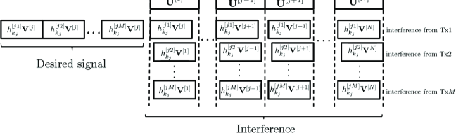
Figure 11: Interference alignment at receiver $j$ under state $k_{j}$

After aligning interference, the equivalent received signal is

$$y^{[j]}_{k_{j}}=A(\sum_{i=1}^{M}h^{[ji]}_{k_{j}}\mathbf{V}^{[j]}\mathbf{X}^{[ji]}+\sum_{l\neq j}\mathbf{U}^{[l]}\mathbf{X}^{[l]})+z^{[j]}_{k_{j}}$$ (209)

where each elements of column vector $\mathbf{X}^{[l]}$ is the sum of all interference along the same direction.

First note that members of $\mathbf{V}^{[1]},\ldots,\mathbf{V}^{[N]}$ are distinct. To show that each data stream can achieve $\frac{1}{m_{n}}$ DoF, we need to check if all elements of $h^{[j1]}_{k_{j}}\mathbf{V}^{[j]},h^{[j2]}_{k_{j}}\mathbf{V}^{[j]},\ldots,h^{[jM]}_{k_{j}}\mathbf{V}^{[j]}$ and $\mathbf{U}^{[1]},\ldots,$ $\mathbf{U}^{[j-1]},\mathbf{U}^{[j+1]},\ldots,\mathbf{U}^{[N]}$ are distinct. It can be seen that elements of $h^{[ji]}_{k_{j}}\mathbf{V}^{[j]}~{}\forall i=1,\ldots,M$ are distinct, since $h^{[ji]}_{k_{j}}$ is not contained in members of $\mathbf{V}^{[j]}$. In addition, $\mathbf{U}^{[l]}~{}\forall l\neq j$ does not have $h^{[li]}_{k_{l}},i=1,2,\ldots,M$ while it is contained in $\mathbf{V}^{[j]}$. Therefore, they are all distinct. Since none of them is equal to 1, the total number of degrees of freedom is

$$d = \frac{M\sum_{j=1}^{N}n^{\Gamma_{j}}}{1+\max_{j}\big{(}Mn^{\Gamma_{j}}+(N-1)(n+1)^{\Gamma_{j}}\big{)}}$$ (210)

almost surely. As $n\rightarrow\infty$, $d=\frac{MN}{M+N-1}$.  

Appendix F Proof of Theorem 6

Proof: The message from transmitter $i$ to receiver $i$ denoted as $W^{[i]}$ is encoded into $n^{\Gamma}$ independent data streams where $\Gamma=(K-1)(J_{1}+\ldots+J_{K})$. Let $X^{[i]}_{k}$ denote the symbol of the $k$th data stream from transmitter $i$. For any $\epsilon>0$, let $\mathcal{C}=\{x:x\in\mathbb{Z}\cap[-P^{\frac{1-\epsilon}{2(m_{n}+\epsilon)}},P^{\frac{1-\epsilon}{2(m_{n}+\epsilon)}}]\}$ where $m_{n}=1+(n+1)^{\Gamma}+n^{\Gamma}$. In other words, $\mathcal{C}$ denotes a set of all integers in the interval $[-P^{\frac{1-\epsilon}{2(m_{n}+\epsilon)}},P^{\frac{1-\epsilon}{2(m_{n}+\epsilon)}}]$. Each symbol in the data stream is obtained by uniformly i.i.d. sampling $\mathcal{C}$.

For transmitter $i=1,\ldots,K$, the transmitted signal is obtained by multiplexing different data streams $X^{[i]}_{k},\forall k=1,\ldots,n^{\Gamma}$ using the same $1\times n^{\Gamma}$ vector $\mathbf{V}$. Note that all elements of $\mathbf{V}$ are functions of channel coefficients which will be designed later. Then, the transmitted signal is

$$x^{[i]} = A\sum_{k=1}^{n^{\Gamma}}V_{k}X^{[i]}_{k}$$ (211)

$$= A\mathbf{V}\mathbf{X}^{[i]}~{}~{}~{}i=1,2,\ldots,K$$ (212)

where $\mathbf{X}^{[i]}=[X^{[i]}_{1}X^{[i]}_{2}\cdots X^{[i]}_{n^{\Gamma}}]^{T}$ and $\mathbf{V}=[V_{1}~{}V_{2}\cdots V_{n^{\Gamma}}]$. $A$ is a scalar which is designed such that the power constraints are satisfied, i.e.,

$$E(x_{i}^{2})\leq P~{}~{}\forall i=1,2,\cdots,M.$$ (213)

Since

$$E(x_{i}^{2})\leq A^{2}P^{\frac{1-\epsilon}{m_{n}+\epsilon}}\|\mathbf{V}\|^{2}\leq P,$$ (214)

we have

$$A=\frac{1}{\|\mathbf{V}\|}P^{\frac{m_{n}-1+2\epsilon}{2(m_{n}+\epsilon)}}$$ (215)

The received signal at receiver $j$ under state $k_{j}$ is given by:

$$y^{[j]}_{k_{j}} = A(\sum_{i=1}^{K}h^{[ji]}_{k_{j}}x^{[i]})+z^{[j]}_{k_{j}}$$ (216)

$$= A(\underbrace{h^{[jj]}_{k_{j}}\mathbf{V}\mathbf{X}^{[j]}}_{\textrm{desired signal}}+\underbrace{\sum_{i\neq j}h^{[ji]}_{k_{j}}\mathbf{V}\mathbf{X}^{[i]}}_{\textrm{interference}})+z^{[j]}_{k_{j}}\$$

In order to get $n^{\Gamma}$ interference free dimensions for the desired signal in a total of $1+n^{\Gamma}+(n+1)^{\Gamma}$ dimension, we align all interference into a $(n+1)^{\Gamma}$ dimensional subspace spanned by members of a $1\times(n+1)^{\Gamma}$ vector $\mathbf{U}$:

$$\left\{\begin{array}[]{ccc}\textrm{span}(h^{[j1]}_{k_{j}}\mathbf{V})&\subset&\textrm{span}(\mathbf{U})\\ &\vdots&\\ \textrm{span}(h^{[j(j-1)]}_{k_{j}}\mathbf{V})&\subset&\textrm{span}(\mathbf{U})\\ \textrm{span}(h^{[j(j+1)]}_{k_{j}}\mathbf{V})&\subset&\textrm{span}(\mathbf{U})\\ &\vdots&\\ \textrm{span}(h^{[jK]}_{k_{j}}\mathbf{V})&\subset&\textrm{span}(\mathbf{U})\end{array}\right.$$ (223)

Equivalently, the above alignment equations can be rewritten as

$$\textrm{span}(h^{[ji]}_{k_{j}}\mathbf{V}) \subset \textrm{span}(\mathbf{U})~{}~{}i,j=1,\ldots,K,~{}i\neq j,~{}k_{j}=1,\ldots,J_{j}$$ (224)

From Lemma 1, we can construct $\mathbf{V}$ and $\mathbf{U}$ as follows:

$$\mathbf{V} = \big{\{}\prod(h^{[ji]}_{k_{j}})^{\alpha^{[ji]}_{k_{j}}}:\forall\alpha^{[ji]}_{k_{j}}\in\{1,2,\ldots,n\},~{}i,j=1,\ldots,K,~{}i\neq j,~{}k_{j}=1,\ldots,J_{j}\big{\}}$$ (225)

$$\mathbf{U} = \big{\{}\prod(h^{[ji]}_{k_{j}})^{\alpha^{[ji]}_{k_{j}}}:\forall\alpha^{[ji]}_{k_{j}}\in\{1,2,\ldots,n+1\},~{}i,j=1,\ldots,K,~{}i\neq j,~{}k_{j}=1,\ldots,J_{j}\big{\}}$$ (226)

Note that $\mathbf{V}$ and $\mathbf{U}$ have $n^{\Gamma}$ and $(n+1)^{\Gamma}$ elements, respectively, where $\Gamma=(K-1)(J_{1}+\ldots+J_{K})$. Now after interference alignment, the received signal is equivalent to

$$y^{[j]}_{k_{j}}=A(h^{[jj]}_{k_{j}}\mathbf{V}\mathbf{X}^{[j]}+\mathbf{U}\bar{\mathbf{X}})+z^{[j]}_{k_{j}}$$ (227)

where $\bar{\mathbf{X}}$ is a $(n+1)^{\Gamma}\times 1$ vector and each element of $\bar{\mathbf{X}}$ is the sum of interference along the same direction. Note that elements of $\mathbf{U}$ do not contain $h^{[jj]}_{k_{j}}$ while elements of $h^{[jj]}_{k_{j}}\mathbf{V}$ have. Therefore, all elements of $h^{[jj]}_{k_{j}}\mathbf{V}$ and $\mathbf{U}$ are distinct. In addition, none of members of $h^{[jj]}_{k_{j}}\mathbf{V}$ and $\mathbf{U}$ is equal to 1. Thus, each user can achieve $\frac{n^{\Gamma}}{1+n^{\Gamma}+(n+1)^{\Gamma}}$ DoF regardless of channel realizations almost surely. As $n\rightarrow\infty$, each user can achieve $\frac{1}{2}$ degrees of freedom almost surely.

References

- [1] S. Jafar and M. Fakhereddin, “Degrees of Freedom for the MIMO interference channel”, IEEE Trans. on Information Theory, vol. 53, No. 7, July. 2007.
- [2] C. Huang, S. Jafar, S. Shamai and S. Vishwanath, “On Degrees of Freedom Region of MIMO Networks without CSIT”, Proceedings of ITA workshop at UC San Diego, 2009 (Full paper available on Arxiv)
- [3] V. Cadambe and S. Jafar, “Interference alignment and the degrees of freedom of the user interference channel”, IEEE Trans. on Information Theory, vol. 54, pp. 3425–3441, Aug. 2008.
- [4] V. Cadambe and S. Jafar, “Interference Alignment and the Degrees of Freedom of Wireless Networks”, IEEE Trans. on Information Theory, vol. 55, No. 9, Sep. 2009.
- [5] G. Caire, N. Jindal and S. Shamai, “On the Required Accuracy of Transmitter Channel State Information in Multiple Antenna Broadcast Channels”, IEEE ACSSC 2007, pp. 287–291, Nov. 2007.
- [6] T. Yoo, N. Jindal and A. Goldsmith,, “Finite-Rate Feedback MIMO Broadcast Channels with a Large Number of Users”, IEEE International Symposium on Information Theory, July 2006.
- [7] N. Jindal, “MIMO Broadcast Channels with Finite Rate Feedback”, IEEE Trans. Information Theory, Vol. 52, No. 11, pp. 5045-5059, Nov. 2006.
- [8] N. Ravindran and N. Jindal, “MIMO Broadcast Channels with Block Diagonalization and Finite Rate Feedback”, IEEE ICASSP, April 2007.
- [9] A. Lapidoth, S. Shamai and M. Wigger, “On the capacity of Fading MIMO broadcast channels with imperfect transmitter side-information”, arXiv:cs/0605079v1, May. 2006.
- [10] H. Weingarten, S. Shamai and G. Kramer, “On the compound MIMO broadcast channel”, Information Theory Workshop, Jan. 2007
- [11] M. Maddah-Ali, A. Motahari, and A. Khandani, “Signaling over MIMO multi-base systems Combination of multi-access and broadcast schemes”, in Proc. IEEE ISIT, 2006, pp. 2104 C2108, June 2006.
- [12] M. Maddah-Ali, A. Motahari, and A. Khandani, “Communication Over Channel: Signaling and Performance Analysis”, Unive.Waterloo,Waterloo, ON, Canada, Tech. Rep. UW-ECE-2006-27, Dec. 2006.
- [13] S. Jafar, S. Shamai, “Degrees of Freedom Region for the MIMO Channel”, IEEE Trans. on Information Theory, vol. 54, No. 1, pp. 151-170, Jan. 2008.
- [14] V. Cadambe, S. Jafar and C. Wang, “ Interference Alignment with Asymmetric Complex Signaling - Settling the Host-Madsen-Nosratinia Conjecture”, e-print, arxiv:0904.0274, April 2009.
- [15] A.S. Motahari, S. O. Gharan and A. K. Khandani, “Real Interference Alignment with Real Numbers,” http://arxiv.org/abs/0908.1208, Aug. 2009.
- [16] R. Etkin and E. Ordentlich, “On the Degrees-of-Freedom of the -User Gaussian Interference Channel”, http://arxiv.org/abs/0901.1695, Jan. 2009.
- [17] T. Gou, S. Jafar, “Degrees of Freedom of the User MIMO Interference Channel”, arxiv:0809.0099, Sept. 2008.
- [18] A.S. Motahari, S. O. Gharan, M.A. Maddah-Ali and A. K. Khandani, “Forming Pseudo-MIMO by Embedding Infinite Rational Dimensions Along a Single Real Line: Removing Barriers in Achieving the DOFs of Single Antenna Systems”, http://arxiv.org/abs/0908.2282, Aug. 2009.
- [19] G. Bresler, A. Parekh and D. Tse, “The approximate capacity of the many-to-one and one-to-many Gaussian interference channels”, http://arxiv.org/abs/0809.3554, 2008.
- [20] V. Cadambe, S. Jafar, and S. Shamai, “Interference Alignment on the Deterministic Channel and Application to Fully Connected Gaussian Interference Networks”, IEEE Transactions on Information Theory, Vol. 55, No. 1, Jan 2009
- [21] V. Cadambe, S. Jafar, “Degrees of Freedom of Wireless Networks - What a Difference Delay Makes”, Proceedings of Asilomar Conference on Signals, Systems and Computers, 2007
- [22] L. Grokop, D. Tse and R. Yates, “Interference Alignment for Line-of-Sight Channels”, arXiv:0809.3035, 2009.