The Clean Way to Identify a Scalar Glueball

Abstract

The existence of a glueball has been a tough work for many years study. Utilizing the well developed QCD theory for $B$ meson decays, we propose a new way to identify whether a scalar glueball existed or not. In the presence of mixing between glueballs and ordinary scalar mesons, we explore the possibility to extract the mixing parameters from semileptonic $B$ decays and nonleptonic $B$ decays. We also point out a clean way to identify a glueball through $B_{c}$ decays.

I Introduction

Quark model has achieved a great success to describe hadronic states, but the QCD also predicts the existence of mesons without any valence quark, which is called glueball. The confirmation of a glueball is one of the most important topics in hadron physics and this subject has received extensive interests rev . Lattice QCD, which is almost the only method to do calculations from the fundamental QCD, predicted that the mass of the lowest-lying scalar glueball ($0^{++}$) is around 1.5-1.8 GeV Bali:1993fb . Several different candidates have been observed in this mass region, but there is not any solid evidence on the existence of a pure glueball. For decades, people have tried to find a way to verify the existence of a glueball through its decay property. The glueball is quark flavor singlet, which should decay to $u\bar{u}$, $d\bar{d}$ and $s\bar{s}$ equally. However, the claimed “unique” feature of quark flavor singlet, is not unique, since the quark-antiquark state can also be flavor SU(3) singlet. Thus, it is not a firm evidence for a glueball. Furthermore, it is very likely that the glueball mix with the quark-antiquark scalar state and they together form several physical mesons. On the theoretical side, there are large ambiguities on the mixing mechanism scalarmesons . This makes the study even more complicated.

Recently, another important direction to uncover the mysterious structure of scalar mesons, is discussed, which investigates the scalar meson production property through $B$ meson decays. In $B$ meson decays, the $O_{8g}$ operator has a large Wilson coefficient, which could produce a number of gluons. These gluons in the final state may have the tendency to form a glueball state, thus the glueball production in inclusive $B$ decays has attracted some theoretical interest Minkowski:2004xf ; He:2006qk . In a recent study first , we calculate the transition form factors of $B$ meson decays into a scalar glueball in the light-cone formalism. Compared with form factors of $B$ to ordinary scalar mesons, the $B$-to-glueball form factors have the same power in the expansion of $1/m_{B}$. Taking into account the leading twist light-cone distribution amplitude, we find that they are numerically only a little smaller than those form factors of $B$ to ordinary scalar mesons. It means that the production rate of glueball in B decays is quite copious.

The scalar meson can be produced in $B$ decays by two gluon (glueball) and also an isosinglet $q\bar{q}$ pair (ordinary meson). In this paper, we will propose a method for experiments to measure the nonzero two gluon contribution, so that to prove the existence of a scalar glueball cleanly. This will require the detection of scalar meson production from $B_{c}$ decays.

II the study of mixing between glueball and quark states

Up to the leading Fock state, a glueball is made up of two constituent gluons. In exclusive $B$ decays, these two gluons can be emitted from either the heavy $b$ quark or the light quark. In the expansion of $\alpha_{s}$, the lowest order Feynman diagrams for form factors of $B$ decays into a scalar glueball are depicted in Fig. 1 (a), (b) and (c). In Fig. 1 (d) and (e), the light antiquark in $B$ meson and the energetic quark from the electro-weak vertex also form an isospin or SU(3) singlet scalar meson. Usually, people believe that the form factor of $B$ decays to an ordinary scalar meson is larger than that of $B$ decays into a scalar glueball. Our recent study shows first that the form factors of $B$ decays into a scalar glueball is big enough for the experiments to observe it. Compared with our previous studies Wang:2006ria ; Li:2008tk on the transition form factors of $B$ mesons decays into ordinary scalar mesons (denoted as $f_{0}$ with the mass around 1.5 GeV), the $B\to G$ form factors are at the same order of magnitude. The $B$-to-glueball form factors are only a factor of two smaller than the $B\to\pi$ form factors. These form factor results are collected in table 1 for comparison . In fact, the main decay channel of a scalar glueball is $\pi\pi$ or $K\bar{K}$. Thus a scalar glueball is much easier to detect than the iso-singlet pseudoscalar meson such as $\eta$. Compared with the recently measured semileptonic $B\to\eta$ decay Aubert:2008ct

$${\cal B}(B^{-}\to\eta l^{-}\bar{\nu}) = (3.1\pm 0.6\pm 0.8)\times 10^{-5},$$ (1)

the branching ratio of $B\to Gl\bar{\nu}$ first is comparable with that of $B\to\eta l\bar{\nu}$ decay and may be observed on the ongoing $B$ factories. It is very likely for the forthcoming Super B factory to observe a pure glueball, if it exists.

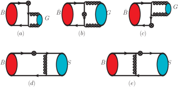
Figure 1: Feynman diagrams of $\bar{B}$ decays into a scalar glueball $G$ and an ordinary scalar meson. The $\otimes$ denotes the possible Lorentz structure arising from the electroweak interactions.

Table 1: $B$ to glueball $(G)$, $B$ to ordinary scalar meson ($f_{0}$) and $B$ to pseudoscalar meson ($\pi$) transition form factors in the PQCD approach

	$F_{0}(0)=F_{1}(0)$	$F_{T}(0)$
$B\to G$	$0.11^{+0.02}_{-0.02}$	$0.05^{+0.01}_{-0.01}$
$B\to\pi$	$0.22^{+0.04}_{-0.05}$	$0.27^{+0.05}_{-0.06}$
$B\to f_{0}$ Scenario I	$-0.30_{-0.09}^{+0.08}$	$-0.39_{-0.11}^{+0.10}$
$B\to f_{0}$ Scenario II	$0.63_{-0.14}^{+0.23}$	$0.76_{-0.17}^{+0.37}$

However, there is not any solid experimental evidence for a pure glueball state up to now. The reason may be that the glueball state can mix with the ordinary meson through the strong interactions. For example, the Lattice QCD collaboration predicted the mass of a scalar glueball ground state around $1.5$-1.8 GeV. It is very likely that the glueball state mix with the ordinary quark-antiquark state and they form several physical mesons. In this mass region, there are three scalar mesons: $f_{0}(1370)$, $f_{0}(1500)$ and $f_{0}(1710)$, which might be the potential candidates. The mixing matrix can be set as

$$\left(\begin{array}[]{c}f_{0}(1710)\\ f_{0}(1500)\\ f_{0}(1370)\end{array}\right)=\left(\begin{array}[]{ccc}a_{1}&a_{2}&a_{3}\\ b_{1}&b_{2}&b_{3}\\ c_{1}&c_{2}&c_{3}\end{array}\right)\left(\begin{array}[]{c}G\\ \bar{s}s\\ \bar{n}n\end{array}\right).$$ (11)

For each physical scalar meson for example $f_{0}(1370)$, which is a mixture of glueball and ordinary states, the coefficients $c_{1}$, $c_{2}$ and $c_{3}$ satisfy the normalization condition

$$\sqrt{|c_{1}|^{2}+|c_{2}|^{2}+|c_{3}|^{2}}=1.$$ (12)

A non-zero $c_{1}$ would be a clear evidence for the existence of a glueball. Let us aim this to see if there is a way to settle it in $B$ decays. The semileptonic $B\to f_{0}l\bar{\nu}$ decays receive contributions from the $\bar{n}n$ component but without $\bar{s}s$ component (at least negligible), while the semileptonic $B_{s}\to f_{0}l^{+}l^{-}$ channel only receive contributions from the $\bar{s}s$ but without $\bar{n}n$ component. Both of the decay channels can receive gluon component contributions. Thus from eq.(12), we notice that the two independent mixing parameters can be fitted from the above two experimental measurements, in principle. For the three kinds of $f_{0}$’s, we have altogether 6 experiments, but only three real parameters in eq.(11) to be fixed. Since the branching fraction of $B_{s}\to f_{0}l^{+}l^{-}$ is expected to have the order of $10^{-8}$ or even smaller, one needs to accumulate a large number of $B$ decay events. This could be achieved on the future experiments such as the Super B factory.

Semileptonic $B$ decays are clean but in $B\to f_{0}l\bar{\nu}$, the neutrino is identified as missing energy and the efficiency is limited; while the $B_{s}\to f_{0}l^{+}l^{-}$ has a small branching ratio. In these decays, the lepton pair does not carry any SU(3) flavor and the decay amplitudes receive less pollution from the strong interactions. The lepton pair can also be replaced by a charmonium state such as $J/\psi$ since $J/\psi$ does not carry any light flavor either. $B\to J/\psi f_{0}$ decays may provide another ideal probe to detect the internal structure of the scalar mesons. In $B\to J/\psi f_{0}$ decay, the $\bar{s}s$ component will not contribute at the leading order in $\alpha_{s}$. For example, the $B\to J/\psi\phi$ decay has been set a very stringent upper limit :2008bt : ${\cal B}(B\to J/\psi\phi)<9.4\times 10^{-7}$. Thus $B\to J/\psi f_{0}$ decay can filter out the glueball component and the $\bar{n}n$ component of a scalar meson. Meanwhile in $B_{s}\to J/\psi f_{0}$ decay, only the $\bar{s}s$ and the gluon component contributes. Moreover, the final mesons in these channels are easy to reconstruct and these channels could have sizable branching fractions. If we use the factorization method, decay amplitudes are given as

$$A(\bar{B}^{0}\to J/\psi f_{0}) = \frac{G_{F}}{\sqrt{2}}V_{cb}V_{cd}^{*}m_{B}^{2}f_{J/\psi}a_{2}F_{1}^{B\to f_{0}}(m_{J/\psi}^{2}).$$

The Wilson coefficient $a_{2}$ can be extracted from the $B\to J/\psi K$ decays Amsler:2008zzb

$${\cal B}(\bar{B}^{0}\to J/\psi\bar{K}^{0}) = (8.71\pm 0.32)\times 10^{-4}.$$ (14)

The branching ratios are roughly predicted as

$${\cal B}(\bar{B}^{0}\to J/\psi f_{0}(\bar{n}n)) \simeq \left\{\begin{array}[]{c}(23^{+12}_{-14})\times 10^{-6}\;\;\;\;\;{\rm S1}\\ (10^{+7}_{-5})\times 10^{-5}\;\;\;\;\;{\rm S2}\end{array}\right.,$$ (17)

$${\cal B}(\bar{B}^{0}\to J/\psi G) \simeq (6.2\pm 2.2)\times 10^{-6},$$ (18)

where we have assumed the same $q^{2}$ dependence for all form factors and $F_{1}^{B\to K}(0)=0.3$. The uncertainties are from the experimental data for ${\cal B}(B\to J/\psi K)$ and the $B\to S$ form factors at the $q^{2}=0$ point. For the $B_{s}$ decays, the branching ratios are comparable with that of $B\to J/\psi K$:

$${\cal B}(\bar{B}_{s}\to J/\psi f_{0}(\bar{s}s)) \simeq \left\{\begin{array}[]{c}(6.5^{+4.0}_{-4.5})\times 10^{-4}\;\;\;\;\;\;\;{\rm S1}\\ (3.5^{+2.3}_{-1.4})\times 10^{-3}\;\;\;\;\;\;\;{\rm S2}\end{array}\right.,$$ (21)

$${\cal B}(\bar{B}_{s}\to J/\psi G) \simeq (9.7\pm 3.9)\times 10^{-5}.$$ (22)

Such large branching fractions offer a great opportunity to probe structures of scalar mesons. With the available data in the future, the mixing problem between the scalar mesons will be solvable and the glueball component can be projected out in principle.

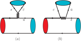
Figure 2: Feynman diagrams of $B\to f_{0}D$ decays.

If the power-suppressed annihilation diagrams are neglected, the charmful decays of $B$ meson, $B\to f_{0}D$, can also be used to constrain the mixing between scalar mesons. For instance in $B^{-}\to D_{s}^{-}f_{0}$, the $\bar{n}n$ and gluon component contribute but the $\bar{s}s$ component does not, while in $\bar{B}_{s}\to D^{0}f_{0}$, the $\bar{n}n$ component will not contribute, as shown in Fig. 2. Thus the mixing coefficients can also be determined if these two channels are experimentally measured. It is necessary to point out that this method may suffer from sizable uncertainties of annihilation diagrams Wang:2006ria .

To be more specific, we will discuss two mixing mechanisms in detail. Because the decay width of $f_{0}(1500)$ is not compatible with the ordinary $\bar{q}q$ state, Amsler and Close claimed that $f_{0}(1500)$ is primarily a scalar glueball Amsler:1995tu . In the subsequent studies, they extracted the mixing matrix through fitting the data of two-body decays of scalar mesons Close:2000yk :

$$\left(\begin{array}[]{c}f_{0}(1710)\\ f_{0}(1500)\\ f_{0}(1370)\end{array}\right)=\left(\begin{array}[]{ccc}0.36&0.93&0.09\\ -0.84&0.35&-0.41\\ 0.40&-0.07&-0.91\end{array}\right)\left(\begin{array}[]{c}G\\ \bar{s}s\\ \bar{n}n\end{array}\right).$$ (32)

Based on the SU(3) assumption for scalar mesons and the quenched LQCD results, Cheng et al. Cheng:2006hu reanalyze all existing experimental data and fit the mixing coefficient as

$$\left(\begin{array}[]{c}f_{0}(1710)\\ f_{0}(1500)\\ f_{0}(1370)\end{array}\right)=\left(\begin{array}[]{ccc}0.93&0.17&0.32\\ -0.03&0.84&-0.54\\ -0.36&0.52&0.78\end{array}\right)\left(\begin{array}[]{c}G\\ \bar{s}s\\ \bar{n}n\end{array}\right).$$ (42)

It is found that the $f_{0}(1710)$ tends to be a primary glueball. This is very different from the first matrix of mixing coefficients in (32). The scalar meson production rates in $B$ meson decays can be used to distinguish these assignments, starting with the $B\to S$ form factors collected in Tab. 1. For example in scenario I, if we use the mixing coefficients in Eq. (32), the production rates of $f_{0}(1710)$ and $f_{0}(1500)$ in $B$ decays are much smaller than that of $f_{0}(1370)$ but they have large and comparable production rates in $B_{s}$ decays; if we use the mixing coefficients in Eq. (42), $f_{0}(1710)$ has small production rates in both $B$ and $B_{s}$ decays but the other two mesons have large and comparable production rates in $B$ and $B_{s}$ decays. Based on our predictions on form factors Wang:2006ria ; Li:2008tk ; first , these differences in $B$ and $B_{s}$ decays are helpful to distinguish the two mixing matrix.

III Glueball production in $B_{c}$ decays

The ordinary light scalar meson is isospin singlet and/or flavor SU(3) singlet, while the glueball is flavor SU(6) singlet. Therefore it is difficult to distinguish them by the light $u$, $d$ and $s$ quark coupling. However, the light ordinary scalar meson has negligible $c\bar{c}$ component, while the glueball have the same coupling to $c\bar{c}$ as that to the $u\bar{u}$, $d\bar{d}$ or $s\bar{s}$. A clean way to identify a glueball is then through the $c\bar{c}$ coupling to the glueball.

In $B$ decays, the initial heavy meson contains a light quark, thus contributions of the gluon component always accompany with the quark content $\bar{n}n$ or $\bar{s}s$. It is not easy to isolate the gluon content. The situation in the doubly-heavy $B_{c}$ meson is different: it contains a heavy charm antiquark. The semileptonic $B_{c}\to f_{0}l\bar{\nu}$ decays would happen only through Fig. 1(a)(b) and (c) but not through Fig. 1(d) and (e). The observation of this decay channel in the experiments will surely establish the existence of a scalar glueball. Moreover the CKM matrix element in this channel is $V_{cb}$, thus the $B_{c}\to f_{0}l\bar{\nu}$ will have a sizable branching ratio. This channel will depend on the $B_{c}\to G$ transition form factor which requires the less-constrained $B_{c}$ meson’s light-cone distribution amplitude. But even if we assume the form factor of $B_{c}\to G$ is smaller than the $B_{c}\to\eta_{c}$ form factor by one order, branching ratios of $B_{c}\to Gl\bar{\nu}(l\bar{\nu})$ are suppressed by two orders

$${\cal B}(B_{c}\to Gl\bar{\nu}) \sim 1\%\times 0.01=10^{-4},$$ (43)

where the branching ratio of $B_{c}\to\eta_{c}l\bar{\nu}$ has been taken as $1\%$. This branching ratio is large enough for the experiments. One only needs to reconstruct the $f_{0}$ scalar meson in the final state and also the $B_{c}$ meson mass in the intermediate state, so that to make sure that the scalar meson is produced from two gluons. That experiment is achievable even if the $f_{0}$ meson is not a pure glueball, but at least has a large portion of it.

$B_{c}\to f_{0}\pi^{-}$ is another potential mode to figure out the gluon content. But in this mode, the $\bar{n}n$ component also contributes through the annihilation diagrams. The $b$ and $\bar{c}$ quark annihilates and the $d$ and $\bar{u}$ quark are created. The CKM matrix element $V_{cb}$ and the Wilson coefficient $a_{1}$ are the same with the emission diagram for the $B_{c}$-to-glueball transition. The offshellnes of the two internal particles in annihilation diagrams are of the order $m_{B_{c}}^{2}$. The electroweak vertex is the $V-A$ type and the decay amplitude is proportional to the light quark mass. Thus the decay amplitudes via annihilation diagram for the $\bar{n}n$ component are expected to be suppressed. As a result, the $B_{c}\to f_{0}\pi^{-}$ also filters out the gluon component of the scalar meson as an approximation.

IV Summary

Although the $B$-to-glueball form factors are small, they can not be neglected and more interestingly these form factors may have different interferences with those for the quark content, according to different descriptions of scalar mesons. If a scalar meson is a mixture of a glueball and an ordinary meson, we investigate the possibility to extract the mixing mechanism from semileptonic $B$ decays. Semileptonic $B\to f_{0}l\bar{\nu}$ and $B_{s}\to f_{0}l^{+}l^{-}$ decays can be used to determine the internal structures. The nonleptonic $B\to J/\psi f_{0}$ and $B_{s}\to J/\psi f_{0}$ decays are also analyzed. To avoid the interference between the quark and the gluon component, we find that the $B_{c}\to f_{0}l\bar{\nu}$ and $B_{c}\to f_{0}\pi^{-}$ will project out the gluon component of a scalar meson cleanly. Our results can be generalized to the other glueballs.

References

- (1) E. Klempt and A. Zaitsev, Phys. Rept. 454, 1 (2007) [arXiv:0708.4016 [hep-ph]]; D. M. Asner et al., arXiv:0809.1869 [hep-ex]; V. Crede and C. A. Meyer, Prog. Part. Nucl. Phys. 63, 74 (2009) [arXiv:0812.0600 [hep-ex]].
- (2) G. S. Bali, et al. [UKQCD Collaboration], Phys. Lett. B 309, 378 (1993); H. Chen, J. Sexton, A. Vaccarino and D. Weingarten, Nucl. Phys. Proc. Suppl. 34, 357 (1994); C. J. Morningstar and M. J. Peardon, Phys. Rev. D 60, 034509 (1999) ; A. Vaccarino and D. Weingarten, Phys. Rev. D 60, 114501 (1999) ; C. Liu, Chin. Phys. Lett. 18, 187 (2001); D. Q. Liu, J. M. Wu and Y. Chen, High Energy Phys. Nucl. Phys. 26, 222 (2002) ; N. Ishii, H. Suganuma and H. Matsufuru, Phys. Rev. D 66, 014507 (2002) ; M. Loan, X. Q. Luo and Z. H. Luo, Int. J. Mod. Phys. A 21, 2905 (2006) ; Y. Chen et al., Phys. Rev. D 73, 014516 (2006) ;
- (3) S. Spanier, N.A. Törnqvist, and C. Amsler, note on scalar mesons, review published on PDG.
- (4) P. Minkowski and W. Ochs, Eur. Phys. J. C 39, 71 (2005) [arXiv:hep-ph/0404194]; P. Minkowski and W. Ochs, arXiv:hep-ph/0304144.
- (5) X. G. He and T. C. Yuan, arXiv:hep-ph/0612108.
- (6) W. Wang, Y.L. Shen and C.D. Lu, e-Print: arXiv:0908.2216 [hep-ph].
- (7) W. Wang, Y. L. Shen, Y. Li and C. D. Lu, Phys. Rev. D 74, 114010 (2006) [arXiv:hep-ph/0609082].
- (8) R. H. Li, C. D. Lu, W. Wang and X. X. Wang, Phys. Rev. D 79, 014013 (2009) .
- (9) B. Aubert et al. [BABAR Collaboration], arXiv:0808.3524 [hep-ex].
- (10) Y. Liu et al. [Belle Collaboration], Phys. Rev. D 78, 011106 (2008) [arXiv:0805.3225 [hep-ex]].
- (11) C. Amsler and F. E. Close, Phys. Lett. B 353, 385 (1995) [arXiv:hep-ph/9505219]; C. Amsler and F. E. Close, Phys. Rev. D 53, 295 (1996) [arXiv:hep-ph/9507326].
- (12) F. E. Close and A. Kirk, Phys. Lett. B 483, 345 (2000) [arXiv:hep-ph/0004241]; F. E. Close and Q. Zhao, Phys. Rev. D 71, 094022 (2005) [arXiv:hep-ph/0504043].
- (13) H. Y. Cheng, C. K. Chua and K. F. Liu, Phys. Rev. D 74, 094005 (2006) [arXiv:hep-ph/0607206].
- (14) C. Amsler et al. [Particle Data Group], Phys. Lett. B 667, 1 (2008).