Pure Phase Decoherence in a Ring Geometry

Abstract

We study the dynamics of pure phase decoherence for a particle hopping around an $N$-site ring, coupled both to a spin bath and to an Aharonov-Bohm flux which threads the ring. Analytic results are found for the dynamics of the influence functional and of the reduced density matrix of the particle, both for initial single wave-packet states, and for states split initially into 2 separate wave-packets moving at different velocities. We also give results for the dynamics of the current as a function of time.

I Introduction

The dynamics of phase decoherence is central to our understanding of those physical systems whose properties depend on interference. This is particularly evident when particles are forced to propagate around closed paths; phase coherence then makes all physical properties depend on the topology of these paths thouless . For this reason the quantum dynamics of particles on rings has been extremely important in our understanding of quantum phase coherence. Examples at the microscopic level include the energetics and response to magnetic fields of molecules orbital , as well as charge transfer dynamics in a vast array of solid-state and biochemical systems. There is evidence now for coherent transport around ring structures even in some large biomolecules LH-2 . At the nanoscopic and mesoscopic scale many ring-like structures, both conducting and superconducting AhB-scond , show coherent transport around the rings, along with interesting Aharonov-Bohm style interference phenomena. We also note the importance of closed loop structures in quantum information processing QIP .

The interference around loops in all of these systems is very sensitive to phase decoherence. Questions about the mechanisms and dynamics of this decoherence are subtle, and have led to major controversies, notably in the discussion of mesoscopic conductors tau-phi . A quantitative understanding of decoherence processes in metallic systems and in superconducting ”qubits” has yet to be attained (in both cases local defect modes clearly make the major contribution to phase decoherence at low temperature $T$ TLS-TauPhi ; TLS-SQUID ). These controversies are examples of a wider problem: typically in solid-state systems, low $T$ decoherence rates are far higher in experiments than theoretical estimates based on the dissipation rates in these systems.

These problems are complex because both decoherence and dissipation rates depend strongly on which environmental modes are causing the decoherence SHPMP ; PS00 . Delocalized modes (electrons, phonons, photons, spin waves, etc.) can typically be modeled as ”oscillator bath” modes feynman63 ; cal83 ; weiss99 . In such models, decoherence goes hand-in-hand with dissipation AJL84 ; cal84 , in accordance with the fluctuation-dissipation theorem. However localized modes (defects, dislocations, dangling bonds, nuclear and paramagnetic impurity spins, etc.), which can be mapped to a ”spin bath” representation of the environment SHPMP ; PS00 , behave quite differently; indeed they often give decoherence with almost no dissipation. This is because although their low characteristic energy scale means they can cause little dissipation, nevertheless their phase dynamics can be strongly affected when they couple to some collective coordinate - this then causes strong decoherence in the dynamics of this coordinate PS00 ; gaita08 . The fluctuation-dissipation theorem is then not obeyed SHPMP , and often these localized modes are rather far from equilibrium.

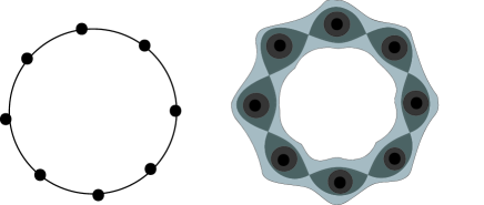
Figure 1: At left, An 8-site ring with nearest-neighbour hopping between sites. At right a potential $U({\bf R})$ with 8 potential wells (shown here symmetric under rotations by $\pi/4$), depicted as a contour map (with lower potential shown darker). When truncated to the 8 lowest eigenstates, this is equivalent to the 8-site model.

To understand how such non-dissipative decoherence processes work, it is then useful to look at models in which the environment causes pure phase decoherence, with no dissipation. As noted above, such models become particularly interesting when the decoherence is acting on systems propagating in ’closed loops’. Models of rings coupled to oscillator baths have already been studied guinea . However such models, in which decoherence is inextricably linked to dissipation, do not capture the largely non-dissipative decoherence processes that dominate many solids at low $T$. On the the other hand pure phase decoherence has been studied in many papersunruh95 ; ekert96 ; milburn05 , but not, as far as we know, the rather unique phenomena occurring on a ring.

In this paper we study a model which embodies in a simple way both the ’closed path’ propagation which is generic to quantum interference processes, and which involves pure phase decoherence coming from a spin bath. The model describes a particle propagating around a ring of $N$ discrete sites, while coupled to a spin bath; we assume hopping between nearest neighbors. The model becomes particularly interesting if we also have a flux $\Phi$ threading the ring (see Fig. 1). The spin bath variables are assumed to be Two-Level Systems (TLS); these are ubiquitous in solid-state systems, and are the main cause of decoherence at low $T$ in these systems.

One can also study the problem of a continuous ring, but the discrete model is simpler, and is easily related to diverse problems like quantum walks with phase decoherence PS06 ; QW-diss , or the dynamics of electrons in rings of quantum dots QDot-ring . The Hamiltonian we will study has the general form

$$H_{\phi}\;=\;\sum_{<ij>}[\Delta_{o}c^{{\dagger}}_{i}c_{j}e^{i(A_{ij}^{o}+\sum_{k}\mbox{\boldmath$\alpha$}_{k}^{ij}\cdot\mbox{\boldmath$\sigma$}_{k})}+H.c.]$$ (1)

The operator $c_{j}^{{\dagger}}$ creates a particle at site $j$; we assume a single particle only. The phase factors $\{A_{ij}^{o}\}$ result from the flux $\Phi$ threading the ring. In writing (1), we have assumed a symmetric ring, with $N$ sites, and assumed that the hopping matrix elements $t_{ij}$ between sites $i$ and $j$ have simplified to a nearest-neighbour amplitude $\Delta_{o}$ (here $\sum_{<ij>}$ denotes a sum over nearest neighbours). This also means we can ignore any diagonal site energies, since symmetry under rotations by angles $2\pi/N$ means these energies are all the same. The spin bath variables $\{\mbox{\boldmath$\sigma$}_{k}\}$ are Pauli spin-$1/2$ operators for the TLS, with $k=1,2,....N_{s}$. We emphasize immediately that these bath spins are, in real situations, often not spins, but instead the 2 lowest levels of localized modes in a solid (for example, as noted above, they could be defects or dangling bonds).

The paper is organized as follows. In section II we discuss the derivation of model Hamiltonians like (1) from more microscopic models, and the approximations which allow us to drop other terms that can also appear in the coupling of a ring particle to a spin bath. In section III we discuss the dynamics of the particle in the absence of the bath - this establishes a number of useful mathematical results. In section IV we show how the dynamics of the reduced density matrix for the particle is derived in the presence of the bath, and give some results for this dynamics. In section V we analyze the dynamics of a pair of interfering wave-packets moving around the ring, showing how pure phase decoherence destroys the interference between them. Finally, in section VI, we summarize our conclusions - since some of the calculations are quite extensive, readers may want to look first at this section for a guide to the main results. The more technical details of the derivations in sections III and IV are given in an Appendix.

II Derivation of Model

Consider first an $N$-site ring system without a bath. In site representation, this typically has a ”bare ring” model Hamiltonian

$$H_{o}\;=\;\sum_{<ij>}\left[t_{ij}c_{i}^{\dagger}c_{j}\>e^{iA_{ij}^{o}}+H.c.\right]+\sum_{j}\varepsilon_{j}c_{j}^{\dagger}c_{j}$$ (2)

This ”1-band” Hamiltonian is the result of truncating, to low energies, a high-energy Hamiltonian of form:

$$H_{V}\;=\;\frac{1}{2M}({\bf P}-{\bf A}({\bf R}))^{2}+U(\mbox{\boldmath$R$})$$ (3)

where a particle of mass $M$ moves in a potential $U(\mbox{\boldmath$R$})$ characterized by $N$ potential wells in a ring array (see again Fig. 1). Then $\varepsilon_{j}$ is the energy of the lowest state in the $j$-th well, and $t_{ij}$ is the tunneling amplitude between the $i$-th and $j$-th wells (which we take here to be nearest neighbours). In path integral language, this tunneling is over a semiclassical ”instanton” trajectory ${\bf R}_{ins}(\tau)$, occurring over a timescale $\tau_{B}\sim 1/\Omega_{0}$ (the ”bounce time” coleman ). Here $\Omega_{0}$ (the ”bounce frequency”) is roughly the small oscillation frequency of the particle in the potential wells. In a semiclassical calculation, the phase $A_{ij}^{o}$ is that incurred along the semiclassical trajectory by the particle, moving in the gauge field ${\bf A}({\bf R})$. For a symmetric ring the site energy $\varepsilon_{j}\rightarrow\varepsilon_{0},\forall j$, and we henceforth ignore it.

Consider now what happens when we couple the particle to a spin bath. The spin bath itself, independent of the ring particle, has the Hamiltonian

$$H_{SB}\;=\;\sum_{k}{\bf h}_{k}\cdot\mbox{\boldmath$\sigma$}_{k}\;+\;\sum_{k,k^{\prime}}V_{kk^{\prime}}^{\alpha\beta}\sigma_{k}^{\alpha}\sigma_{k^{\prime}}^{\beta}$$ (4)

in which each TLS has some local field ${\bf h}_{k}$ acting on it, and the interactions $V_{kk^{\prime}}^{\alpha\beta}$ are typically rather small because the TLS represent localized modes in the environment. The most general coupling between the ring particle and the bath has the form

$$H_{int}\;=\; \sum_{k}^{N_{s}} [\;\sum_{j}\mbox{\boldmath$F$}_{j}^{k}(\mbox{\boldmath$\sigma$}_{k})\hat{c}_{j}^{\dagger}\hat{c}_{j}$$

$$+ \sum_{<ij>}(\mbox{\boldmath$G$}_{ij}^{k}(\mbox{\boldmath$\sigma$}_{k})\hat{c}_{i}^{\dagger}\hat{c}_{j}+H.c.)]$$ (5)

in which both the diagonal coupling $\mbox{\boldmath$F$}_{j}^{k}$ and the non-diagonal coupling $\mbox{\boldmath$G$}_{ij}^{k}$ are vectors in the Hilbert space of the $k$-th bath spin. We shall see below, when considering the origin of these terms from microscopic models, that very often we can write the total Hamiltonian as

$$H\;=\;H_{band}+H_{SB}$$ (6)

where $H_{band}=H_{o}+H_{int}$ takes the form

$$H_{band}= \sum_{ij}[t_{ij}c_{i}^{\dagger}c_{j}e^{iA_{ij}^{o}+i\sum_{k}(\mbox{\boldmath$\phi$}_{k}^{ij}+\mbox{\boldmath$\alpha$}_{k}^{ij}\cdot\mbox{\boldmath$\sigma$}_{k})}+H.c.]$$ (7)

$$+\;\sum_{j}(\varepsilon_{j}+\sum_{k}\mbox{\boldmath$\gamma$}_{k}^{j}\cdot\mbox{\boldmath$\sigma$}_{k})c_{j}^{\dagger}c_{j}$$

in which the diagonal couplings to the spin bath assume a ”Zeeman” form, of strength $|\mbox{\boldmath$\gamma$}_{k}^{j}|$, linear in the $\{\mbox{\boldmath$\sigma$}_{k}\}$, and the non-diagonal couplings appear in the form of extra phase factors in the hopping amplitude between sites.

Before we consider the microscopic origins of this model, let us note how it simplifies when we assume the symmetry under rotations by $2\pi/N$ noted above (so that the site energy $\varepsilon_{j}$ is dropped, and $t_{ij}\rightarrow\Delta_{o}$, with nearest-neighbour hopping only). It is then natural to write $A_{ij}^{o}$ as

$$A_{ij}^{o}=\frac{e}{2}{\bf H}\cdot{\bf R}_{i}\times{\bf R}_{j}\;=\;\Phi/N$$ (8)

for $j=i+1$ (we now use MKS units, and put $\hbar=1$). Here, ${\bf H}$ is the magnetic field, and ${\bf R}_{i}$ is the radius-vector to the $i$th site; in cylindrical coordinates

$${\bf R}_{j} =(R_{o},\Theta_{j})$$

$$\Theta_{j} =2\pi j/N$$ (9)

for a ring of radius $R_{o}$. Fourier transforming from the site basis to a momentum basis for the couplings, we define quasi-momenta $k_{n}=2\pi n/N$, with $n=0,1,2,...,N-1$, for the particle on the ring, and define operators

$$c^{\dagger}_{j} =\sqrt{\frac{1}{N}}\sum_{k_{n}}e^{ik_{n}j}c^{\dagger}_{k_{n}}\ ,$$

$$c^{\dagger}_{k_{n}} =\sqrt{\frac{1}{N}}\sum_{\ell}e^{-ik_{n}\ell}c^{\dagger}_{\ell}\ ,$$

$$k_{n} =\frac{2\pi n}{N}\ ,\ \ n=0,1,\ldots,N-1\ .$$ (10)

We can write the free particle Hamiltonian as

$$H_{o} = \sum_{n}\epsilon^{o}_{k_{n}}c^{\dagger}_{k_{n}}c_{k_{n}}$$ (11)

$$= 2\Delta_{o}\sum_{n}\cos(k_{n}-\Phi/N)c^{\dagger}_{k_{n}}c_{k_{n}}\$$

Then in this basis we can write:

$$V_{int}=\sum_{k}^{N_{s}}\sum_{n}\left[\mbox{\boldmath$F$}^{k}_{n}(\mbox{\boldmath$\sigma$}_{k})\rho({k_{n}})\;+\;\mbox{\boldmath$G$}_{n}^{k}(\mbox{\boldmath$\sigma$}_{k})\hat{c}_{k_{n}}^{\dagger}\hat{c}_{k_{n}}\right]$$ (12)

where $\rho({k_{n}})=\sum_{n^{\prime}}\hat{c}_{k_{n}+k_{n^{\prime}}}^{\dagger}\hat{c}_{k_{n^{\prime}}}$ is the density operator in momentum space for the particle, and the Fourier-transformed interaction functions are

$$\mbox{\boldmath$G$}_{n}^{k}(\mbox{\boldmath$\sigma$}_{k}) = \sum_{ij}e^{ik_{n}(i-j)}\mbox{\boldmath$G$}^{k}_{ij}(\mbox{\boldmath$\sigma$}_{k})$$

$$\mbox{\boldmath$F$}_{n}^{k}(\mbox{\boldmath$\sigma$}_{k}) = \sum_{j}e^{i{k_{n}}j}\mbox{\boldmath$F$}^{k}_{j}(\mbox{\boldmath$\sigma$}_{k})$$ (13)

In this basis the band Hamiltonian $H_{band}$ has a dispersion which is a functional of the bath spin distribution:

$$H_{band}=\sum_{k}\sum_{n} \epsilon_{k_{n}}[\mbox{\boldmath$\sigma$}_{k}]\hat{c}_{k_{n}}^{\dagger}\hat{c}_{k_{n}}$$

$$+\;\sum_{n,n^{\prime}}v_{n}[\mbox{\boldmath$\sigma$}_{k}]\hat{c}_{k_{n}+k_{n^{\prime}}}^{\dagger}\hat{c}_{k_{n^{\prime}}}$$ (14)

and in which the ’band energy’ $\epsilon_{k_{n}}[\mbox{\boldmath$\sigma$}_{k}]$ and the ’scattering potential’ $v_{n}[\mbox{\boldmath$\sigma$}_{k}]$ are now both functionals over the spin bath coordinates $\{\mbox{\boldmath$\sigma$}_{k}\}$:

$$\epsilon_{k_{n}}[\mbox{\boldmath$\sigma$}_{k}] = \epsilon_{k_{n}}^{o}+\sum_{k}\mbox{\boldmath$G$}_{n}^{k}(\mbox{\boldmath$\sigma$}_{k})$$

$$v_{n}[\mbox{\boldmath$\sigma$}_{k}] = \sum_{k}\mbox{\boldmath$F$}_{n}^{k}(\mbox{\boldmath$\sigma$}_{k})$$ (15)

Under many circumstances one can assume that this symmetry under rotations also applies to the bath couplings, so these no longer depend on site variables, ie., $\mbox{\boldmath$F$}_{j}^{k}\rightarrow\mbox{\boldmath$F$}^{k}$, and $\mbox{\boldmath$G$}_{ij}^{k}\rightarrow\mbox{\boldmath$G$}^{k}$. The results then simplify a great deal; $\mbox{\boldmath$G$}_{n}^{k}(\mbox{\boldmath$\sigma$}_{k})\rightarrow 2\mbox{\boldmath$G$}^{k}(\mbox{\boldmath$\sigma$}_{k})\cos k_{n}$, and $\mbox{\boldmath$F$}_{n}^{k}\rightarrow\mbox{\boldmath$F$}^{k}$.

Now let us consider the microscopic origin of this model (ie., before truncation to the lowest band). The most obvious interaction between the particle moving around the ring and a set of bath spins has the local form dube98 :

$$H_{int}({\bf R},\mbox{\boldmath$\sigma$}_{k})\;=\; \sum_{k}\mbox{\boldmath$F$}(\mbox{\boldmath$R$}-\mbox{\boldmath$r$}_{k})\cdot\mbox{\boldmath$\sigma$}_{k}$$

$$\;\equiv\; \sum_{k}H_{int}^{k}({\bf R},\mbox{\boldmath$\sigma$}_{k})$$ (16)

where $\mbox{\boldmath$F$}(\mbox{\boldmath$r$})$ is some vector function, and $\mbox{\boldmath$r$}_{k}$ is the position at the $k$-th bath spin. The diagonal coupling $\mbox{\boldmath$F$}_{j}^{k}$, or its linearized form $\mbox{\boldmath$\gamma$}_{k}^{j}$, is then easily obtained from (16) when we truncate to the single band form. But the term (16) must also generate a non-diagonal term, which is more subtle. We can see this by defining the operator

$$\hat{T}_{ij}^{k}\;=\;\exp{[-i/\hbar\;\int_{\tau_{in}({\bf R}_{i})}^{\tau_{f}({\bf R}_{j})}d\tau\;H_{int}^{k}({\bf R},\mbox{\boldmath$\sigma$}_{k})]}$$ (17)

where the particle is assumed to start in the $i$-th potential well centered at position ${\bf R}_{i}$, at the initial time $\tau_{in}$, and finish at position ${\bf R}_{j}$ in the adjacent $j$-th well at time $\tau_{f}$; the intervening trajectory is the instanton trajectory (which in general is modified somewhat by the coupling to the spin bath). Now we operate on $\mbox{\boldmath$\sigma$}_{k}$ with $\hat{T}_{ij}^{k}$, to get

$$|\mbox{\boldmath$\sigma$}^{f}_{k}\rangle\;=\;\hat{T}_{ij}^{k}\;|\mbox{\boldmath$\sigma$}^{in}_{k}\rangle\;=\;e^{i(\phi_{k}^{ij}+\mbox{\boldmath$\alpha$}_{k}^{ij}\cdot\mbox{\boldmath$\sigma$}_{k})}|\mbox{\boldmath$\sigma$}^{in}_{k}\rangle$$ (18)

where we note that both the phase $\phi_{k}^{ij}$ multiplying the unit Pauli matrix $\sigma_{k}^{0}$, and the vector $\mbox{\boldmath$\alpha$}_{k}^{ij}$ multiplying the other 3 Pauli matrices $\sigma_{k}^{x},\sigma_{k}^{y},\sigma_{k}^{z}$, are in general complex. In this way the instanton trajectory of the particle acts as an operator in the Hilbert space of the $k$-th bath spin PS00 ; PS93 . Note that one important implication of this derivation is that typically $|\mbox{\boldmath$\alpha$}_{k}^{ij}|\ll 1$, in fact exponentially small, since the interaction energy scale set by $|\mbox{\boldmath$F$}(\mbox{\boldmath$R$}-\mbox{\boldmath$r$}_{k})|$ is usually much smaller than the ”bounce energy” scale $\hbar\Omega_{o}$ set by the potential $U({\bf R})$, ie., the tunneling of the particle between wells is a sudden perturbation on the bath spins PS00 . Detailed calculations in specific cases PS93 ; PS00 ; TPS96 show that $|\mbox{\boldmath$\alpha$}_{k}^{ij}|\sim\pi|\mbox{\boldmath$\omega$}_{k}^{ij}|/2\Omega_{o}$ in this ’sudden’ regime, where $\mbox{\boldmath$\omega$}_{k}^{ij}=\mbox{\boldmath$\gamma$}_{k}^{j}-\mbox{\boldmath$\gamma$}_{k}^{i}$ is the change in the diagonal coupling acting between the particle and the $k$-th bath spin when the particle hops from site $i$ to site $j$ (this result can be found directly from time-dependent perturbation theory in the sudden approximation).

From these considerations we see that, starting from a ring with the particle-bath interaction given in (16), we will end up with an effective Hamiltonian for the lowest band of the form given in (7), in which the non-diagonal interaction $\mbox{\boldmath$G$}_{ij}^{k}(\mbox{\boldmath$\sigma$}_{k})$ in (5) has assumed a rather special form.

One can in fact have a more general form for $\mbox{\boldmath$G$}_{ij}^{k}(\mbox{\boldmath$\sigma$}_{k})$ in the lowest-band approximation, provided one also introduces in the microscopic Hamiltonian a coupling

$$H_{int}({\bf P},\mbox{\boldmath$\sigma$}_{k})\;=\;\sum_{k}\mbox{\boldmath$G$}(\mbox{\boldmath$P$},\mbox{\boldmath$\sigma$}_{k})$$ (19)

to the momentum of the particle. This can include various terms, including functions of $\mbox{\boldmath$P$}\times\mbox{\boldmath$\sigma$}_{k}$ and $\mbox{\boldmath$P$}\cdot\mbox{\boldmath$\sigma$}_{k}$; a detailed analysis is fairly lengthy. The main new effect of these is to generate terms in the band Hamiltonian which couple the spins to the amplitude of $t_{ij}$ as well as to its phase; these do not appear in (7).

In any case, if we know $U(\mathbf{R})$, $\mbox{\boldmath$F$}(\mbox{\boldmath$R$}-\mbox{\boldmath$r$}_{k})$, and $\mbox{\boldmath$G$}(\mbox{\boldmath$P$},\mbox{\boldmath$\sigma$}_{k})$, we can clearly then calculate all the parameters in the generic model Hamiltonian, using various methods PS00 ; TPS96 . However we are not interested here in the generic case, since our main object is to study the dynamics of decoherence in a ring model which contains only phase decoherence. We therefore make the following approximations:

(i) We drop the interaction $V_{kk^{\prime}}^{\alpha\beta}$, between bath spins (often a very good approximation, since interactions between defects or nuclear spins are often very weak), and also neglect the local fields $\mbox{\boldmath$h$}_{k}$ acting on the $\{\mbox{\boldmath$\sigma$}_{k}\}$. Thus we make $H_{SB}=0$.

(ii) We drop the momentum coupling $\mbox{\boldmath$G$}(\mbox{\boldmath$P$},\mbox{\boldmath$\sigma$}_{k})$ entirely, and in the band Hamiltonian (7) we drop the diagonal interaction $\mbox{\boldmath$\gamma$}_{k}^{j}$. This implies that the energy of the $k$-th bath spin does not depend on whether the $j$-th site is occupied. We make this approximation (in many cases not physically reasonable) only because we wish to study phase decoherence without the complication of energy relaxation.

(iii) We assume a symmetric ring, so that $\varepsilon_{j}\rightarrow 0$ and $t_{ij}\rightarrow\Delta_{o}$ as before; and we absorb the phases $\phi_{k}^{ij}\rightarrow\phi_{k}$ into a renormalization of $\Delta_{o}$ (from $\sum_{k}\mbox{Im}\;\phi_{k}$), and of $A^{o}_{ij}$ (from $\sum_{k}\mbox{Re}\;\phi_{k}$).

The resulting model $H_{\phi}$ is then just that given in (1). This turns out to be explicitly solvable, and reveals some important properties of phase decoherence. We will usually assume the parameters $\mbox{\boldmath$\alpha$}_{k}^{ij}$ are small, in line with the remarks above (although the net effect of all of them may be very large), and we will also usually specialize to the case $\mbox{\boldmath$\alpha$}_{k}^{ij}\rightarrow\mbox{\boldmath$\alpha$}_{k}$, consistent with a completely symmetric ring.

Finally, let us briefly compare with the kind of Hamiltonian one would expect for a particle on a ring coupled to an oscillator bath. Let us assume a set of oscillators with Hamiltonian $H_{o}+H_{osc}+H_{int}$, where $H_{o}$ is again the free particle hopping Hamiltonian, coupling to a set of $N_{o}$ oscillators with Hamiltonian

$$H_{osc}=\sum_{q=1}^{N_{o}}{1\over 2}({p_{q}^{2}\over m_{q}}+m_{q}\omega_{q}^{2}x_{q}^{2})\\$$ (20)

In general there will be diagonal couplings $\{V_{j}(q)\}$ and non-diagonal couplings $\{U_{ij}(q)\}$ between particle and oscillators. We could also have a coupling to the oscillator momenta - however in this case one can make a canonical transformationajl84 which transforms this back into a coupling to the $\{x_{q}\}$. Typically the couplings $\{V_{j}(q),U_{ij}(q)\}\sim O(N_{o}^{-1/2})$. We note here that in many microscopic models of this kind, the couplings $\{V_{j}(q),U_{ij}(q)\}$ are actually also strong functions of temperature, either because the underlying effective Hamiltonian is strongly $T$-dependent (eg., in a superconductor amb83 ), or because the coupling to the oscillators is non-linear (eg., in the coupling to a soliton wada78 ).

If we restrict the problem to rotationally invariant couplings on the ring, then we can write

$$H_{int}=\sum_{q}\left[\sum_{<ij>}(U_{q}\hat{c}_{i}^{\dagger}\hat{c}_{j}+H.c.)+\sum_{j}V_{q}\hat{c}_{j}^{\dagger}\hat{c}_{j}\right]x_{q}$$ (21)

where $U_{ij}(q)\rightarrow U_{q}$, $V_{j}(q)\rightarrow V_{q}$, and the sum $\sum_{<ij>}$ is over nearest neighbours. It is then straightforward to go through the same manipulations as in (12)-(15), to get a renormalised band which is a functional of the $\{x_{q}\}$.

In these results there is no connection between the ring sites and the space in which the oscillators are supposed to exist. However in many cases the oscillator displacement field $x_{j}$ can be defined at each site $j$ of the ring; the coupling then reduces to

$$\hat{V}\;=\; \sum_{\bf q}\sum_{j}v_{\bf q}\hat{c}_{j}^{\dagger}\hat{c}_{j}e^{i{\bf q}\cdot{\bf R}_{j}}x_{\bf q}$$

$$\equiv\; \sum_{jj^{\prime}}v({\bf R}_{j}-{\bf r}_{j^{\prime}})\hat{c}_{j}^{\dagger}\hat{c}_{j}x({\bf r}_{j^{\prime}})$$ (22)

in which ${\bf R}_{j}$, ${\bf r}_{j^{\prime}}$ are site vectors on the ring, and $x_{\bf q}$ is now the Fourier transform of $x_{j}$.

III Free band particle Dynamics

We first consider the dynamics of a free particle in some initial state moving on the symmetric $N$-site ring described by $H_{o}$ in (11), with no bath.

For this free particle the dynamics is entirely described in terms of the bare 1-particle Green function

$$G^{o}_{jj^{\prime}}(t) \equiv\langle j|G^{o}(t)|j^{\prime}\rangle\equiv\langle j|e^{-i{\cal H}_{o}t}|j^{\prime}\rangle$$

$$=\frac{1}{N}\sum_{n}e^{-i2\Delta_{0}t\cos(k_{n}-\Phi/N)}e^{ik_{n}(j^{\prime}-j)}\ ,$$ (23)

which gives the amplitude for the particle to propagate from site $j^{\prime}$ at time zero to site $j$ at time $t$. These paths are rather simple (see Fig. 2); they can be labelled by the initial and final sites, and by the winding number of the path around the ring.

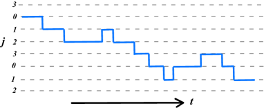
Figure 2: Colour online: A particular path in a path integral for the particle, shown here for an $N=3$ ring. This path, from site $0$ to site $1$, has winding number $p=1$.

The 1-particle Green function can be evaluated in various ways (see Appendix); the result can be usefully written as

$$G^{o}_{jj^{\prime}}(t)=\sum_{p=-\infty}^{+\infty}J_{Np+j^{\prime}-j}(2\Delta_{o}t)e^{-i(Np+j^{\prime}-j)(\Phi/N+\pi/2)}$$ (24)

where $\sum_{p}$ is a sum over winding numbers. The ”return amplitude” $G^{o}_{00}(t)$ is then given by

$$G^{o}_{00}(t) =\sum_{p}e^{-ip\Phi}(-i)^{|Np|}J_{|Np|}(2\Delta_{o}t)$$

$$=\sum_{p}e^{-ip\Phi}I_{Np}(-2i\Delta_{o}t)$$ (25)

where in the last form we use the hyperbolic Bessel function.

It is often more useful to have expressions for the density matrix; even though these depend trivially for a free particle on the Green function, they are essential when we come to compare with the reduced density matrix for the particle coupled to the bath. One has, for the ’bare’ density matrix operator of the system at time $t$,

$$\hat{\rho}^{o}(t)=e^{-i{\cal H}_{o}t}\hat{\rho}^{o}(0)e^{i{\cal H}_{o}t}.$$ (26)

Thus, suppose we have an initial density matrix $\rho^{(in)}_{ll^{\prime}}=\langle l|\rho(t=0)|l^{\prime}\rangle$ (where $l$ and $l^{\prime}$ are site indices), then at a later time $t$ we have

$$\rho^{o}_{jj^{\prime}}(t)\equiv\langle j|\hat{\rho}^{o}(t)|j^{\prime}\rangle =\langle j|e^{-i{\cal H}_{o}t}|l\rangle\rho_{ll^{\prime}}^{(in)}\langle l^{\prime}|e^{i{\cal H}_{o}t}|j^{\prime}\rangle$$

$$=\rho_{ll^{\prime}}^{(in)}G^{o}_{jl}(t)G^{o}_{j^{\prime}l^{\prime}}(t)^{\dagger},$$ (27)

where we use the Einstein summation convention (summing over $l,l^{\prime}$). This equation defines the propagator $K^{o}_{jj^{\prime},ll^{\prime}}(t)$ for the free particle density matrix, as

$$K^{o}_{jj^{\prime},ll^{\prime}}(t)=G^{o}_{jl}(t)G^{o}_{j^{\prime}l^{\prime}}(t)^{\dagger}.$$ (28)

In the main text of this paper we will almost always quote results for the special case where the particle begins at $t=0$ on site $0$. In the case of the free particle, this means that $\rho_{ll^{\prime}}^{(in)}=\delta_{0l}\delta_{l^{\prime}0}$, and only the propagator matrix $K^{o}_{jj^{\prime},00}(t)$ enters the results; then we have

$$\langle j|\hat{\rho}^{o}(t)|j^{\prime}\rangle\rightarrow K^{o}_{jj^{\prime},00}(t)=G^{o}_{j0}(t)G^{o}_{j^{\prime}0}(t)^{\dagger}.$$ (29)

In the Appendix we give the results for an arbitrary initial density matrix.

The evaluation of the time-dependent density matrix for the free particle turns out to be quite interesting mathematically. As discussed in the Appendix, one can evaluate $\rho^{o}_{jj^{\prime}}(t)$ as a sum over pairs of paths in a path integral, to give a double sum over winding numbers, or else as a single sum over winding numbers. Consider first the double sum form; again, for the special case where $\rho^{(in)}_{ll^{\prime}}=\delta_{0l}\delta_{l^{\prime}0}$ (the particle starts at the origin), this can be written as

$$\rho^{o}_{jj^{\prime}}(t)=\sum_{pp^{\prime}}e^{i(p-p^{\prime})\Phi}e^{i\Phi(j-j^{\prime})/N}(-i)^{Np+j}(i)^{Np^{\prime}+j^{\prime}}J_{Np+j}(2\Delta_{o}t)J_{Np^{\prime}+j^{\prime}}(2\Delta_{o}t),$$ (30)

where $p,p^{\prime}$ are the winding numbers (see Appendix for the derivation for a general initial density matrix). This form has a simple physical interpretation - the particle propagates along pairs of paths in the density matrix, one finishing at site $j$ and the other at site $j^{\prime}$, and the order of each Bessel function simply gives the total number of sites traversed in each path, with appropriate Aharonov-Bohm phase multipliers for each path.

If one instead writes the answer as a single sum over winding numbers, again assuming $\rho^{(in)}_{ll^{\prime}}=\delta_{0l}\delta_{l^{\prime}0}$, we get:

$$\rho^{o}_{jj^{\prime}}(t)=\frac{1}{N}\sum_{m=0}^{N-1}\sum_{p^{\prime}=-\infty}^{\infty}J_{Np^{\prime}+j^{\prime}-j}[4\Delta_{o}t\sin(k_{m}/2)]e^{i\Phi[p^{\prime}+(j^{\prime}-j)/N]-ik_{m}(j+j^{\prime}-Np^{\prime})/2}\$$ (31)

where as before the $\{k_{m}\}$ are the momenta of the particle eigenfunctions. The physical interpretation of this form is less obvious, but the sums are much easier to evaluate since they only contain single Bessel functions instead of pairs of them. Thus wherever possible we reduce double sum forms to single sums. Notice that for these finite rings, the bare density matrix is of course strictly periodic in time. Notice also that the diagonal elements of $\rho(t)$ are generally periodic in $\Phi$. However, the off-diagonal elements are only periodic in $\Phi/N$. In contrast, $e^{i\Phi(j-j^{\prime})/N}\langle j|\rho(t)|j^{\prime}\rangle$ is periodic in $\Phi$, with period $2\pi$. This latter is the quantity needed for calculating the currents, as we will see below.

From either $G^{o}_{jj^{\prime}}(t)$ or $\rho^{o}_{jj^{\prime}}(t)$ we may immediately compute two useful physical quantities. First, the probability $P^{o}_{j0}(t)$ to find the particle at time $t$ at site $j$, assuming it starts at the origin; and second, the current $I^{o}_{j,j+1}(t)$ between adjacent sites as a function of time.

Looking first at the probability $P^{o}_{j0}(t)$, one has

$$P^{o}_{j0}(t)=\langle j|\hat{\rho}^{o}(t)|j\rangle=|G^{o}_{j0}(t)|^{2}$$ (32)

which from above can be written in double sum form as

$$P^{o}_{j0}(t)= \sum_{pp^{\prime}}J_{Np+j}(2\Delta_{o}t)J_{Np^{\prime}+j}(2\Delta_{o}t)$$

$$\;\;\;\;\;\;\;\;\;\times\;e^{-iN(p^{\prime}-p)(\Phi/N+\frac{\pi}{2})}$$ (33)

or in single sum form as

$$P^{o}_{j0}(t)= \frac{1}{N}\sum_{m=0}^{N-1}\sum_{p=-\infty}^{\infty}e^{ip(\Phi+Nk_{m}/2)}$$

$$\times J_{Np}[4\Delta_{o}t\sin(k_{m}/2)]\ .$$ (34)

One may also compute moments of these probabilities. These are not terribly meaningful for a small ring, because any wave-packet will be spread around the ring. However for a large ring they can be useful- for example, the 2nd moment $\sum_{j}j^{2}P^{o}_{j0}(t)$ tells us the rate at which an initial density matrix spreads in time, provided the spatial extent of the density matrix is much smaller than the ring circumference. Coherent dynamics will then manifest itself as ballistic propagation of an initial wave-packet.

From these general expressions it is hard to see what is going on. To give some idea of how the probability density behaves, it is useful to then look at these results for a small 3-site ring, where the oscillation periods are quite short. One then has, for the case where the particle starts at the origin, that

$$P^{o}_{j0}(t)=\frac{1}{3}\bigl{(}1+(3\delta_{j,0}-1)\bigl{[}J_{0}(2\Delta_{o}\sqrt{3}t)$$

$$+2\sum_{p=1}^{\infty}J_{6p}(2\Delta_{o}\sqrt{3}t)\cos(2p\Phi)\bigr{]}$$

$$+(\delta_{j,1}-\delta_{j,2})2\sqrt{3}\sum_{p=1}^{\infty}J_{6p-3}(2\Delta_{o}\sqrt{3}t)\sin((2p-1)\Phi)\bigl{)}\ .$$ (35)

In Fig. 3 the return probability $P^{o}_{00}(t)$ is plotted for the case $N=3$, using (35). From the results one striking feature immediately emerges - we see that the periodic behaviour depends strongly on the flux $\Phi$. This flux dependence illustrates the way in which the flux controls the particle dynamics, by acting directly on the particle phase. In section V we will see how this also happens when one looks at interference between 2 wave-packets; and in sections IV and V we will see how decoherence washes out the flux dependence of the particle dynamics. Thus the flux dependence of the particle dynamics very effectively measures how coherent its dynamics may be.

Turning now to the current $I^{o}_{j,j+1}(t)$ from site $j$ and site $j+1$, this is given from elementary quantum mechanics by

$$I^{o}_{j,j+1} (t)\;\;=\;\;2\;{\rm Im}\;[\Delta_{o}e^{-i\Phi/N}\rho^{o}_{j,j+1}(t)]$$

$$=\;\;i\Delta_{o}\Bigl{(}e^{i\Phi/N}\rho^{o}_{j+1,j}(t)-e^{-i\Phi/N}\rho^{o}_{j,j+1}(t)\Bigr{)}$$ (36)

where the flux per link appears in each contribution. Again, one can write this expression as either a double sum over pairs of winding numbers, or as a single sum (see Appendix for the general results and derivation). For the case where the particle starts from the origin, these expressions reduce to

$$I^{o}_{j+1,j}\;= \;2\Delta_{o}\sum_{pp^{\prime}}J_{Np+j}(2\Delta_{o}t)J_{Np^{\prime}+j+1}(2\Delta_{o}t)\cos[(\frac{\pi}{2}N+\Phi)(p^{\prime}-p)]$$

$$= \;\frac{2\Delta_{o}}{N}\sum_{m=0}^{N-1}\sum_{p}J_{Np+1}(4\Delta_{o}t\sin\frac{k_{m}}{2})e^{-ik_{m}(\frac{Np+1}{2}+j)}i^{Np+1}\cos[(\frac{\pi}{2}N+\Phi)p]$$ (37)

for the double and single sum forms respectively.

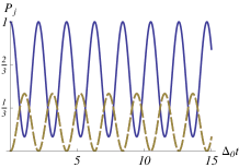
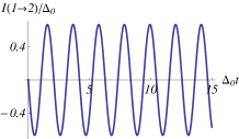
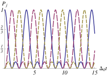
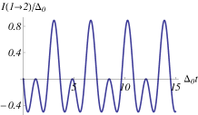
Figure 3: Colour online: Results for the free particle for $N=3$ and for a particle initially on site $1$. Left: The probabilities to occupy site $1$ (full line), $2$ (large dashes), and $3$ (small dashes). Right: the current from site $1$ to site $2$. Top: $\Phi=0$. Bottom: $\Phi=\pi/2$.

Again, the currents across any links must be strictly periodic in time for this free particle system; and again, it is useful to show the results for a 3-site system. For this case $N=3$, and assuming that the particle begins at the origin, we find

$$\begin{split}I^{o}_{0,1}\;=\;\frac{2\Delta_{o}}{3}&{\rm Im}\sum_{m=1}^{2}\sum_{p}J_{3p+1}(4\Delta_{o}t\sin\frac{m\pi}{3})\\ &\times e^{-im\pi(3p+1)/3}i^{3p+1}\cos[(\frac{3\pi}{2}+\Phi)p]\end{split}$$ (38)

which we can also write in the form

$$I^{o}_{0,1}\;=\; \frac{2\Delta_{o}}{3}{\rm Im}\sum_{p}J_{3p+1}(2\sqrt{3}\Delta_{o}t)\cos[(\frac{3\pi}{2}+\Phi)p]$$

$$\times i^{3p+1}\sum_{m=1}^{2}(e^{-i\pi(3p+1)/3}+e^{-i2\pi(3p+1)/3})$$ (39)

Now let us write $(e^{-i\pi(3p+1)/3}+e^{-i2\pi(3p+1)/3})=(-1)^{p}e^{-i\pi/3}+e^{-2i\pi/3}$. If $p$ is even, this becomes $-i\sqrt{3}$ and $\cos[(\frac{3\pi}{2}+\Phi)p]=(-1)^{3p/2}\cos(\Phi p)$; If $p$ is odd, it becomes $-1$ and $\cos[(\frac{3\pi}{2}+\Phi)p]=(-1)^{3(p-1)/2}\sin(\Phi p)$. Therefore, we have

$$I^{o}_{0,1}= \frac{2}{3}\Delta_{o}\sum_{p=-\infty}^{\infty}J_{3p+1}(2\Delta_{o}\sqrt{3}t)K(p,\Phi)\ ,$$

$$K(p,\Phi)=\sin(p\Phi)\ \ \ {\rm if}\ \ p={\rm odd}\ ,$$

$$K(p,\Phi)=\sqrt{3}\cos(p\Phi)\ \ \ {\rm if}\ \ p={\rm even}\ .$$ (40)

These results are also shown in Fig. 3. Notice that in this special case the result is periodic in $\Phi$; this is not however true for a general initial density matrix $\rho^{(in)}_{ll^{\prime}}$, when the result is periodic in $\Phi/N$.

IV Ring plus Bath: Phase Averaging

We now wish to solve for the dynamics of the particle once it is coupled to the bath, via the Hamiltonian (1). This is done in general by integrating out the bath spins, to produce expressions for the reduced density matrix of the particle. In this section we first show how this is done, and then give results for physical quantities (in particular, the probability $P_{j0}(t)$ and the current $I_{j,j+1}(t)$). Finally, we briefly compare the results to the behaviour one expects for a ring coupled to an oscillator bath.

IV.1 General results

As shown in the Appendix, the reduced density matrix for the particle obeys the equation of motion

$$\rho_{jj^{\prime}}(t)=\sum_{l,l^{\prime}}{\cal K}_{jj^{\prime},ll^{\prime}}(t)\rho^{(in)}_{l,l^{\prime}}$$ (41)

where ${\cal K}_{jj^{\prime},ll^{\prime}}(t)$ is the propagator for the reduced density matrix. This latter can be written in the form of a double sum over winding numbers

$${\cal K}_{jj^{\prime},ll^{\prime}}(t)=\sum_{pp^{\prime}}K^{o}_{jj^{\prime},ll^{\prime}}(p,p^{\prime};t)F_{jj^{\prime}}^{ll^{\prime}}(p,p^{\prime})$$ (42)

where the function $K^{o}_{jj^{\prime},ll^{\prime}}(p,p^{\prime};t)$ is the free particle propagator for fixed winding numbers $p,p^{\prime}$ (so that $K^{o}_{jj^{\prime},ll^{\prime}}(t)=\sum_{pp^{\prime}}K^{o}_{jj^{\prime},ll^{\prime}}(p,p^{\prime};t)$; see the Appendix, eqtn. (82) et seq.). All effects from the spin bath are then contained in $F_{jj^{\prime}}^{ll^{\prime}}(p,p^{\prime})$, which we will call the ”influence function”. The remarkable thing is that this function depends only on the initial and final states, and on the winding numbers - all other aspects of the two paths involved in the density matrix propagation have disappeared. As explained in the appendix, this is a particular feature of the pure phase decoherence being treated here.

The form the influence function takes depends on what kind of averaging we do over the bath. To discuss this, let us first discriminate between two different ways of averaging over the bath, as follows:

(i) The first and most obvious case is where the $\mbox{\boldmath$\alpha$}_{k}^{mn}$ are considered to be a set of fixed couplings, for a specific single ring. In this case the average is only over the bath states; we will denote this bath average by $<....>$. Often it will only involve a thermal average over the bath states.

(ii) However it is often the case that one is either interested in an ensemble of rings, all having the same free particle Hamiltonian but with the $\mbox{\boldmath$\alpha$}_{k}$ possibly varying from one ring to another, or a single ring in which the values of the couplings $\mbox{\boldmath$\alpha$}_{k}$ are indeterminate. In this case it makes sense to define a probability distribution $P(\mbox{\boldmath$\alpha$})$ over a coupling variable $\alpha$. One then must average not only over the bath states themselves, but also over the bath couplings. We will denote this double average by $<<.....>>$, to signify the average over both the bath states and the probability distribution; and the influence function for this case will be written as $\bar{F}_{jj^{\prime}}^{ll^{\prime}}(p,p^{\prime})$, with the bar over the $F$ signifying that an average over couplings is being done as well.

In general the results for the dynamics of the density matrix and the current, and their dependence on the influence function, may be quite complicated. Thus, before we begin quoting results, it is useful to note what are the important parameters in the problem. We will only consider here the simplest completely symmetric case where $\mbox{\boldmath$\alpha$}_{k}^{mn}\rightarrow\mbox{\boldmath$\alpha$}_{k}$ for all links $\{mn\}$; and we will assume that $|\mbox{\boldmath$\alpha$}_{k}|\ll 1$ for all $k$, as discussed in section II. Now in the previous literature for this case of pure phase decoherence, it has been usual to define a ’topological decoherence’ parameter PS00 ; PS93

$$\lambda\;=\;\frac{1}{2}\sum_{k}|\mbox{\boldmath$\alpha$}_{k}|^{2}$$ (43)

which provides a measure of the strength of the pure phase decoherence PS00 . If the number $N_{s}$ of bath spins is large, then we can have $\lambda\gg 1$; this is the limit of strong phase decoherence.

However we shall see in what follows that on a ring it is often more useful to define a parameter $F_{0}(\bar{p})$ that also depends on a winding number $\bar{p}$. The form of this parameter depends on which of the two bath averages is performed. In the case where only an average over the bath states is performed, we have

$$F_{0}(\bar{p})\;=\;\prod_{k}\cos(N\bar{p}|\mbox{\boldmath$\alpha$}_{k}|)$$ (44)

which defines a rather complicated function of the fixed bath couplings. The strong decoherence limit for this case is defined by the parameter $\lambda$ defined above.

In the case where we also perform an average over the bath couplings, we have

$$\bar{F}_{0}(\bar{p})=\prod_{k}\int d\mbox{\boldmath$\alpha$}_{k}P(\mbox{\boldmath$\alpha$}_{k})\cos(N\bar{p}|\mbox{\boldmath$\alpha$}_{k}|)$$ (45)

The result then depends on what form one has for the distribution function $P(\mbox{\boldmath$\alpha_{k}$})$. In what follows we will use, as an example, a Gaussian distribution, given by

$$P(|\mbox{\boldmath$\alpha$}_{k}|)=e^{-|\mbox{\boldmath$\alpha$}_{k}|^{2}/2\lambda_{o}}/\sqrt{2\pi\lambda_{o}}$$ (46)

so that

$$\bar{F}_{0}(\bar{p})=e^{-\lambda N^{2}\bar{p}^{2}/2},\ \ \ \ \lambda=N_{s}\lambda_{o}\$$ (47)

The limit $\lambda\rightarrow\infty$ is the “strong decoherence” limit for this distribution, where we have $\bar{F}_{0}(\bar{p})\rightarrow\delta_{\bar{p},0}$. However we will see below that it is convenient to think of the strong decoherence regime for the present problem as that for which the particle dynamics is independent of flux - we will see that this happens already for quite small values of $\lambda$.

We can see why these functions enter by considering the forms for $F_{jj^{\prime}}^{ll^{\prime}}(p,p^{\prime})$ and $\bar{F}_{jj^{\prime}}^{ll^{\prime}}(p,p^{\prime})$ that enter into physical quantities. In the appendix the full expressions for these are derived; but here we will again only use them for the case where $\rho^{(in)}_{l,l^{\prime}}=\delta_{0l}\delta_{l^{\prime}0}$, ie., the particle starts at the origin, and so only the function $F_{jj^{\prime}}(p,p^{\prime})\equiv F_{jj^{\prime}}^{00}(p,p^{\prime})$ comes in. We will also again assume the purely symmetric case where $\mbox{\boldmath$\alpha$}_{k}^{ij}\rightarrow\mbox{\boldmath$\alpha$}_{k}$ for every link.

Let us first consider the case of fixed bath couplings. In this case the form of the influence function reduces to (see Appendix):

$$F_{jj^{\prime}}(p,p^{\prime})\;=\;\langle e^{-iN[(p-p^{\prime})+(j-j^{\prime})]\sum_{k}\mbox{\boldmath$\alpha$}_{k}\cdot\mbox{\boldmath$\sigma$}_{k}}\rangle$$ (48)

Notice that $F_{jj^{\prime}}(p,p^{\prime})$ is a function only of the distance $j-j^{\prime}$ between initial and final sites, and of the difference $\bar{p}=p-p^{\prime}$ in winding numbers. Writing this now as $F_{jj^{\prime}}(\bar{p)}$, let us evaluate it by assuming the usual thermal initial bath spin distribution. Since all the bath states are degenerate, then at any finite $T$ all states are equally populated; we then get:

$$F_{jj^{\prime}}(\bar{p})\;=\;\prod_{k}\cos((N\bar{p}+j-j^{\prime})|\mbox{\boldmath$\alpha$}_{k}|)$$ (49)

Other initial non-thermal distributions for the spin bath states are also easily evaluated from (48).

IV.2 Physical Quantities

From expressions like (49) one can now write down expectation values of physical quantities as a function of time. The simplest example is the probability for the particle to end up at some site after a time $t$, having started at another. Thus, eg., the probability $P_{j0}(t)$ to move to site $j$ from the origin in time $t$ is now given by

$$P_{j0}(t)\;=\; \rho_{jj}(t)$$

$$= \;\sum_{pp^{\prime}}J_{Np+j}(2\Delta_{o}t)J_{Np^{\prime}+j}(2\Delta_{o}t)$$

$$\;\;\;\;\times e^{-iN(p^{\prime}-p)(\Phi/N+\frac{\pi}{2})}\;F_{0}(p,p^{\prime})$$ (50)

which is a simple generalization of the free particle result in (33); we note that only the term

$$F_{0}(p,p^{\prime})\;=\;\prod_{k}\cos(N(p-p^{\prime})|\mbox{\boldmath$\alpha$}_{k}|)$$ (51)

in the influence function survives in this expression. Since this function depends only on the difference $p-p^{\prime}$, it is identical to the function $F_{0}(\bar{p})$ defined in (44) above (letting $p=\bar{p}$). We shall see below that the ring current is also controlled by this same function. Note that it has a complex multiperiodicity, as a function of the $N_{s}$ different parameters $N\bar{p}|\mbox{\boldmath$\alpha$}_{k}|$; we do not have space here to examine the rich variety of behaviour found in the system dynamics as we vary these parameters.

Now let us consider the case where we also average over the bath couplings. One then finds (see appendix) that

$$\bar{F}_{jj^{\prime}}(\bar{p})=\prod_{k}\int d\mbox{\boldmath$\alpha$}_{k}P(\mbox{\boldmath$\alpha$}_{k})\langle e^{-iN[\bar{p}+(j-j^{\prime})]\mbox{\boldmath$\alpha$}_{k}\cdot\mbox{\boldmath$\sigma$}_{k}}\rangle$$ (52)

In the symmetric case we can treat each bath spin in the same way, and simply use a distribution function $P(|\mbox{\boldmath$\alpha$}|)$, the same for all the different $\{\mbox{\boldmath$\sigma$}_{k}\}$. Then we can treat everything in terms of this single average, over a single representative spin $\sigma$ from the bath. Then, eg., for an initial thermal ensemble for the bath spins, this gives

$$\bar{F}_{jj^{\prime}}(\bar{p})=[\int d\mbox{\boldmath$\alpha$}P(\mbox{\boldmath$\alpha$})\cos((N\bar{p}+j-j^{\prime})|\mbox{\boldmath$\alpha$}|)]^{N_{s}}$$ (53)

To give something of the flavour of this case, we use the Gaussian distribution for the $P(|\mbox{\boldmath$\alpha$}|)$, given by (46) above. Then, for the thermal ensemble just given, we have

$$\bar{F}_{jj^{\prime}}(\bar{p})=\exp[-\lambda(N\bar{p}+j^{\prime}-j)^{2}/2]$$ (54)

It is then immediately obvious that the result for the probability for the particle to go from site $0$ to site $j$ in time $t$ is the same expression as (50) above, but now with $\bar{F}_{0}(\bar{p})$ instead of $F_{0}(\bar{p})$.

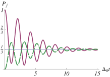
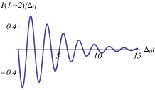
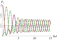
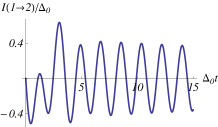
Figure 4: Colour online: Plot of $P_{j0}(t)$ for a $3$-site ring, for a particle initially on site $1$, in the intermediate decoherence limit, with $\lambda=.02$. Left: The probability to occupy site $0$ (full line), $1$ (large dashes), and $2$ (small dashes). Right: the current from site $0$ to site $1$. Top: $\Phi=0$. Bottom: $\Phi=\pi/2$ .

To see how this behaves, let us take the specific case where $N=3$ again. Then for this 3-site ring one has, for example, that

$$P_{10}(t)=\frac{1}{3} \bigl{(}1+2[J_{0}(2\Delta_{o}\sqrt{3}t)$$

$$+2\sum_{p=1}^{\infty}J_{6p}(2\Delta_{o}\sqrt{3}t)\cos(2p\Phi)\bar{F}_{0}(6p)]\bigr{)}\ .$$ (55)

To analyse this result, note that for $x\gg(6p)^{2}$, we can use $J_{6p}(x)\approx(-1)^{p}\sqrt{2/(\pi x)}\cos(x-\pi/4)$. The function ${\bar{F}}_{0}({\bar{p}})$ decays with ${\bar{p}}$, and becomes negligible for large enough ${\bar{p}}$. For example, Eqtn. (47) implies that ${\bar{F}}_{0}(6p)<e^{-10}$ for ${\bar{p}}>p_{max}$, with $p_{max}=\sqrt{5/9\lambda}$. Neglecting these terms in the sum in Eq. (55) we conclude that for $2\Delta_{o}\sqrt{3}t\gg(6p_{max})^{2}$ we have e.g.

$$P_{10}(t) \approx\frac{1}{3}\bigl{[}1+\frac{2A}{\sqrt{\pi\Delta_{o}\sqrt{3}t}}\cos(2\Delta_{o}\sqrt{3}t-\pi/4)\bigr{]}\ ,$$

$$A=1+2\sum_{p=1}^{\infty}(-1)^{p}\cos(2p\Phi)\bar{F}_{0}(6p)\ .$$ (56)

The sum in the amplitude $A$ reduces to $\sum(-1)^{p}\bar{F}_{0}(6p)$, for $\Phi=0$, and to $\sum\bar{F}_{0}(6p)$, for $\Phi=\pi/2$. Clearly, switching from $\Phi=0$ to $\Phi=\pi/2$ causes a large increase in $A$. Notice that the inverse Fourier transform of the amplitude $A(\phi)$ can be used to measure the decoherence function $\bar{F}_{0}(6p)$. Results for this low decoherence regime are shown in Fig. 4.

As $\lambda$ increases, $p_{max}$ decreases, and Eq. (56) applies at shorter times. Remarkably, if $\lambda>0.1$ the whole sum becomes negligible, and we have already reached the strong decoherence result where the result is $\Phi-$independent. The result is shown in Fig. 5. Thus, if we define the ’strong decoherence’ regime as that where all results are flux-independent, then it is reached for very low values of $\lambda$. We emphasize here that the detailed form of the results, as well as the decoherence strength required for flux-independent dynamics, depends strongly on the form we adopt for either $F_{0}(p)$ or $\bar{F}(p)$; we do not have space to explore this question here.

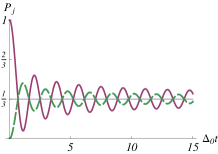
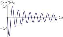
Figure 5: Colour online: Plot of $P_{j0}(t)$ for a $3$-site ring, for a particle initially on site $1$, in the strong decoherence limit. Left: The probability to occupy site $0$ (full line), $1$ (large dashes), and $2$ (small dashes). Right: the current from site $0$ to site $1$ (compare Fig. 3). The results do not depend on $\Phi$.

Turning now to the current through the ring, we generalize the free particle results in the same way as above. Quite generally one has

$$I_{j,j+1}(t)\;=\;i\langle\tilde{\Delta}_{j,j+1}\rho_{j+1,j}(t)-\tilde{\Delta}_{j+1,j}\rho_{j,j+1}(t)\rangle$$ (57)

where we average the operator

$$\tilde{\Delta}_{j,j+1}=\Delta_{o}e^{i\Phi/N}e^{i\sum_{k}\mbox{\boldmath$\alpha$}_{k}^{j,j+1}\cdot\mbox{\boldmath$\sigma$}_{k}}$$ (58)

over bath states, with fixed bath couplings - the case where one also averages over an ensemble of bath couplings is a by now obvious generalization of this. This expression is evaluated in detail in the Appendix; as noted there, the result is more complicated than it seems, because the density matrix depends implicitly on both the initial state, and on the full details of the propagator for the density matrix. Here we consider only the special case where the particle starts from the origin, and the fully symmetric case $\mbox{\boldmath$\alpha$}_{k}^{ij}\rightarrow\mbox{\boldmath$\alpha$}_{k}$. Then one has, for the case of a bath state average only, that

$$I_{j,j+1}(t)\;=\;\frac{2\Delta_{o}}{N}\sum_{m=0}^{N-1}\sum_{p}J_{Np+1}(4\Delta_{o}t\sin\frac{k_{m}}{2})e^{-ik_{m}(\frac{Np+1}{2}+j)}i^{Np+1}F_{0}(p)\cos[(\frac{\pi}{2}N+\Phi)p]$$ (59)

with a similar result for the current $\bar{I}_{j,j+1}(t)$ arising in the case where one also averages over bath couplings, with $F_{0}(p)$ then replaced by $\bar{F}_{0}(p)$. One can also analyze this result as a function of time, and of the decoherence strength, the ring size, and the flux - there is no space for this here. To nevertheless give some flavour for the results, consider again the 3-site ring, for the coupling averaged case, in the strong decoherence limit. Current then only flows in regions where the initial density matrix is inhomogeneous; for some general initial density matrix one finds

$$\bar{I}_{j,j+1}(t)\rightarrow\frac{2\sqrt{3}}{3}\Delta_{o}(\rho^{(in)}_{j,j}-\rho^{(in)}_{j+1,j+1})J_{1}(2\Delta_{o}\sqrt{3}t)\ ,$$ (60)

where $\rho^{(in)}_{ll^{\prime}}$ is the initial density matrix. Again we see that the result is completely independent of the flux.

IV.3 Comparison with Oscillator Bath

To gain some perspective on the results just given, it is useful to compare with what one might expect for a ring particle coupled to an oscillator bath. The differences are both formal and physical, and both are important. Here we simply sketch these - a more detailed study of this rather complex problem will appear elsewhere zhen3 . To specify the formal problem completely, one needs first to define ’spectral functions’ for the couplings between the oscillator bath and the ring particle cal83 . These couplings were defined earlier, in (21); Fourier transforming them in the same way as we did for the spin bath couplings, we then define the spectral functions as:

$$J_{\bf p}^{\perp}(\omega)= {\pi\over 2}\sum_{q}{U_{q}^{2}({\bf p})\over\omega_{q}}\delta(\omega-\omega_{q})$$

$$J_{\bf p}^{\parallel}(\omega)= {\pi\over 2}\sum_{q}{V_{q}^{2}({\bf p})\over\omega_{q}}\delta(\omega-\omega_{q})$$ (61)

In many cases the non-diagonal function $J_{\bf p}^{\perp}(\omega)$ can be neglected compared to the diagonal $J_{\bf p}^{\parallel}(\omega)$, and we will assume this here. $J_{\bf p}^{\parallel}(\omega)$ can take many forms; the most commonly analysed is the ”Ohmic form”, where $J_{\bf p}^{\parallel}(\omega)=\eta\omega$ at low frequency, but this form is very useful for systems coupled to an itinerant electron bath, it is inappropriate for insulating systems (where a more accurate low-$\omega$ form is the ”superOhmic” form $J_{\bf p}^{\parallel}(\omega)\sim\omega^{k}$, with $k>1$). In addition, there is often significant low-energy structure in $J_{\bf p}^{\parallel}(\omega)$, not describable by a simple power-law form; and in many cases $J_{\bf p}^{\parallel}(\omega)$ also depends strongly on temperature $T$.

Defining the influence functional ${\cal F}[\Theta,\Theta^{\prime}]$ in the usual way for general paths $\Theta(t),\Theta^{\prime}(t)$ (cf. eqtn. (93) of the Appendix), we can write

$${\cal F} [\Theta,\Theta^{\prime}]=\;\exp{iN^{2}\over\hbar}\int dt_{1}\int dt_{2}\;\times$$

$$[\dot{\varphi}(t_{1})D_{\bf p}(t_{1}-t_{2})\dot{\varphi}(t_{2})+i\Gamma_{\bf p}(t_{1}-t_{2})\dot{\varphi}(t_{1})\dot{\psi}(t_{1})]$$ (62)

where we have defined the sum and difference angular variables

$$\psi(t)= \;(\Theta(t)+\Theta^{\prime}(t))/2$$

$$\varphi(t)= \;(\Theta(t)-\Theta^{\prime}(t))/2$$ (63)

and the oscillator propagator ${\cal D}_{\bf p}(t)=D_{\bf p}(t)+i\Gamma_{\bf p}(t)$, with

$$D_{\bf p}(t)=\; {4\over N^{2}}\int d\omega\;{J_{\bf p}^{\parallel}(\omega)\over\omega^{2}}(1-\cos\omega t)\coth({\beta\hbar\omega\over 2})$$

$$\Gamma_{\bf p}(t)=\; {4\over N^{2}}\int d\omega\;{J_{\bf p}^{\parallel}(\omega)\over\omega^{2}}\sin\omega t$$ (64)

The behaviour in time of $D_{\bf p}(t)$ can be quite complex, and varies strongly with the form of $J_{\bf p}(\omega)$, and with temperature; the details of this behaviour have been reviewed extensively weiss99 ; ajl87 .

In the same way as for the spin bath, we may now construct expressions for the reduced density matrix, and physical correlation functions derived therefrom, by summing over all paths; this is done in a simple generalisation of methods developed for the spin-boson ajl87 and Schmid schmid83 ; mpaf85 models. For example, the probability $P_{n0}(t)$ takes the form

$$P_{n0}(t)\;=\;\sum_{p=-\infty}^{\infty}\sum_{l=|n+Np|}^{\infty}(-1)^{l-n-Np}e^{i\Phi(p+n/N)}\Delta_{o}^{2l}\int_{0}^{t}dt_{2l}\int_{0}^{t_{2l}}...\int_{0}^{t_{1}}\sum_{\{q_{r}\}}\sum_{\{\sigma_{r}\}}F(\{q_{r}\},\{\sigma_{r}\};\{t_{l}\})$$ (65)

written as a sum over winding numbers $p$ and the number of intersite hops $l$. In this expression the influence functional has now become a function $F(\{\xi_{r}\},\{\chi_{r}\};\{t_{l}\})$ of the times $t_{l}$ at which the particle hops, and of two sets of ’charges’ $\{q_{r}\}=\pm 1$, $\{\sigma_{r}\}=\pm 1$. These charges are defined in terms of the sum and difference paths by

$$\psi(t)=\; {\pi\over N}\sum_{r=1}^{l}q_{r}\theta(t-t_{r})$$

$$\varphi(t)=\; {\pi\over N}\sum_{r=1}^{l}\sigma_{r}\theta(t-t_{r})$$ (66)

so that the $q_{r}$ describe hops in the ’centre of mass’ part of the density matrix, and the $\sigma_{r}$ are hops in the ’difference’ or off-diagonal elements of the density matrix. The general form of $F(\{\xi_{r}\},\{\chi_{r}\};\{t_{l}\})$ is

$$F( \{\xi_{r}\},\{\chi_{r}\};\{t_{l}\})\;=\;\delta(2n-\sum_{r=1}^{2l}q_{r})\;\delta(\sum_{r=1}^{2l}\sigma_{r})$$

$$\times\;\exp{i\over\hbar}\sum_{r^{\prime}<r}[D_{\bf p}(t_{r}-t_{r^{\prime}})q_{r}\sigma_{r^{\prime}}+i\Gamma(t_{r}-t_{r^{\prime}})\sigma_{r}\sigma_{r^{\prime}}]$$ (67)

and we get the well-known oscillator-mediated interactions between the charges, familiar from the spin-boson and Kondo problems. Thus from the formal point of view, for a ring particle coupled to either an oscillator or spin bath, the principal difference between the two cases is the existence, in the oscillator bath case, of retarded interactions between particle hops at different times, whose form depends on $J_{\bf p}^{\parallel}(\omega)$ and on $T$. Just as in the spin-boson and Schmid models, the interactions between the charges in the Ohmic case eventually cause a zero temperature Kosterlitz-Thouless binding transition between the charges, which localizes the particle at one site in the ring. This happens at a critical Ohmic coupling strength $\eta\rightarrow\eta_{c}=\hbar/2\pi$, independent of the ring size zhen3 . When $\eta<\eta_{c}$, the particle dynamics is strongly diffusive - we do not go here into the details of how the dynamics varies with $\eta$, with $N$, and with temperature $T$. In the superOhmic case there is no localization transition, no matter how strong the coupling; the analysis of this case is very lengthy zhen3 .

None of these features has any formal counterpart in the coupling to a spin bath. In the present case the spin bath results are entirely independent of $T$, because all bath levels are degenerate. Even when this is not the case (ie., when we add back the local fields $\{{\bf h}_{k}\}$, so that the decoherence becomes temperature dependent), the only way that interactions can be generated between different bath spins is through their coupling to the particle itself - there is no analogue to the propagator ${\cal D}_{\bf p}(t)$.

The key physical difference between this ring-oscillator bath model, and the ring coupled to a spin bath, is that in the oscillator bath system, decoherence is in a certain sense a mere side effect of the dissipation taking place each time the particle excites an oscillator. On the other hand in the spin bath model, no such dissipation occurs, only phase decoherence. This difference is most obviously seen in the centre of mass dynamics of a particle wave-packet - for the oscillator bath model a wave-packet initially moving around the ring will dissipate centre of mass momentum (formally this happens via the interactions between $q_{r}$ and $\sigma_{r^{\prime}}$ in the influence function), slowly bringing it to rest. However, as we see in the next section, for a ring particle coupled to a spin bath, the centre of mass momentum of a wave-packet is completely conserved, even in the strong decoherence limit, provided the spin bath dynamics is governed by its coupling to the ring particle (the typical case). This leads to some counter-intuitive features, as we now see.

V Wave-Packet Interference

It is interesting to now turn to the situation where two signals are launched at $t=0$ from 2 different points in the ring. The idea is to see how the spin bath affects their mutual interference, and how, by effectively coupling to the momentum of the particle, it destroys the coherence between states with different momenta. We do not give complete results here, but only enough to show how things work.

We therefore start with two-wave-packets which will initially be in a pure state, and will then gradually be dephased by the bath. In the absence of a bath, we will assume the wave function of this state to be the symmetric superposition

$$\Psi(t)={1\over\sqrt{2}}(\psi_{1}(t)+\psi_{2}(t))$$ (68)

where the two wave-packets are assumed to have Gaussian form:

$$|\psi_{1}(t)\rangle= {1\over Z} \sum_{n=0}^{N-1}e^{-(k_{n}-\pi/2)^{2}D/2}$$

$$\times e^{-ij_{0}k_{n}-i2\Delta_{0}t\cos(k_{n}-\Phi/N)}|k_{n}\rangle$$ (69)

$$|\psi_{2}(t)\rangle= \frac{1}{Z} \sum_{n=0}^{N-1}e^{-(k_{n}-\pi/2)^{2}D/2}$$

$$\times e^{-i2\Delta_{0}t\cos(k_{n}-\Phi/N)}|2\pi-k_{n}\rangle$$ (70)

where we assume the usual symmetric ring with flux $\Phi$, and $Z=\sqrt{\sum_{n=0}^{N-1}e^{-(k_{n}-\pi/2)^{2}D}}$ is the wave-function normalization factor. At $t=0$, one of the packets is centred at the origin, and the other at site $j_{o}$, and they both have width $D$. Note that the velocity of each wave-packet is conserved, and at times such that $\Delta_{o}t=2n$, they cross each other. From (69) we see that the main effect of the flux is to shift the relative momentum of the wave-packets. It also affects the rate at which the wave-packets disperse in real space - this dispersion rate is at a minimum when $\Phi/N=\frac{\pi}{2}$.

The free-particle wave function in real space is then

$$\begin{split}|\Psi_{j}(t)\rangle=&\frac{1}{Z\sqrt{2N}}\sum_{n=0}^{N-1}e^{-(k_{n}-\pi/2)^{2}D/2}\\ &\times(e^{i(j-j_{0})k_{n}}e^{-2i\Delta_{o}t\cos{(k_{n}+\Phi/N)}}\\ &\;\;\;\;+e^{-ijk_{n}}e^{-2i\Delta_{o}t\cos{(k_{n}-\Phi/N)}})|j\rangle\end{split}$$ (71)

so that the probability to find a particle at time $t$ on site $j$ is $P(j)=|\Psi_{j}(t)|^{2}$.

Let us now consider the effect of phase decoherence from the spin bath. Using the results for $P_{jj^{\prime}}(t)$ from the last section, with an initial reduced density matrix

$$\rho^{(in)}_{jj^{\prime}}\;=\;|\Psi_{j}(t=0)\rangle\langle\Psi_{j^{\prime}}(t=0)|$$ (72)

we find a rather lengthy result for the probability that the site $j$ is occupied at time $t$:

$$\begin{split}P_{j}(t)={1\over 2NZ^{2}}\sum_{n,n^{\prime}=0}^{N-1}\sum_{m=-\infty}^{+\infty}&e^{-((k_{n}-\pi/2)^{2}+(k_{n^{\prime}}-\pi/2)^{2})D/2}F_{0}(m)\\ \times&\{e^{i(j-j_{0})(k_{n}-k_{n^{\prime}})}J_{m}(4\Delta_{o}t\sin{((k_{n}-k_{n^{\prime}})/2)})e^{im((k_{n}+k_{n^{\prime}})/2+\Phi/N)}+\\ &+e^{-i(k_{n}-k_{n^{\prime}})j}J_{m}(4\Delta_{o}t\sin{((k_{n}-k_{n^{\prime}})/2)})e^{im((k_{n}+k_{n^{\prime}})/2-\Phi/N)}+\\ &+[e^{i((j-j_{0})k_{n}+jk_{n^{\prime}})}J_{m}(4\Delta_{o}t\sin{((k_{n}+k_{n^{\prime}})/2)})e^{im((k_{n}-k_{n^{\prime}})-\Phi/N)}+H.c.]\}\end{split}$$ (73)

One can also, in the same way, derive results for the current in the situation where we start with 2 wave-packets. We see that expressions like (73) are too unwieldy for simple analysis. However in the strong decoherence limit (73) simplifies to:

$$P_{j}(t)={1\over 2NZ^{2}} \sum_{n,n^{\prime}=0}^{N-1}e^{-((k_{n}-\pi/2)^{2}+(k_{n^{\prime}}-\pi/2)^{2})D/2}\{e^{i(j-j_{0})(k_{n}-k_{n^{\prime}})}J_{0}(4\Delta t\sin{((k_{n}-k_{n^{\prime}})/2)})+$$

$$+e^{-ij(k_{n}-k_{n^{\prime}})}J_{0}(4\Delta t\sin{((k_{n}-k_{n^{\prime}})/2)})+[e^{i((j-j_{0})k_{n}+jk_{n^{\prime}})}J_{0}(4\Delta t\sin{((k_{n}+k_{n^{\prime}})/2)})+H.c.]\}$$ (74)

and again we see that the flux has disappeared from this equation.

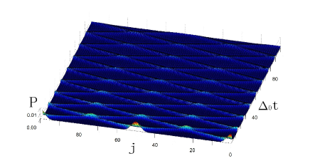
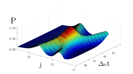
Figure 6: Colour online: Plot for $P_{j}(t)$ as a function of both $j$ and $\Delta_{o}t$ in the strong decoherence limit. $j_{o}=50$ and $N=100$. The relative velocity is $\frac{\pi}{2}$, in phase units. Top: global view. Bottom: a particular peak

This result is shown in Fig. 6. As one might expect, the interference between the two wave-packets is completely washed out in this strong decoherence limit. However there is also a more unexpected feature - each wave-packet now has portions moving in opposite directions to each other. The explanation is to be found by noticing that as the particle hops, at the same time causing the bath spins to make transitions, the topological phase it exchanges with the spins also changes the total phase around the ring seen by the particle. Thus, from the point of view of the particle, these transitions are forcing the total flux through the ring to fluctuate, in a way which depends on the trajectory followed by the particle. This dependence, such that the changing phase is conditional on the particle path, is of course why we get decoherence. Now the changing effective flux changes the particle momentum and velocity, and in the case of the pair of wave-packets here, it also changes their relative momentum. Indeed, given that the transformation $\Phi\rightarrow\Phi+\pi$ completely reverses the momentum, we see that a strong coupling to the bath spins can even cause a part of the initial wave-packets to reverse its direction. However we emphasize that the centre of mass momentum for the combined wave-packet system has not changed - the average momentum imparted to the ring particle is zero. Thus, as noted in the last section, the decoherence caused by the bath is not accompanied by any net dissipation of the particle momentum, or of its energy. Indeed, if a wave-packet starts off with a net angular momentum around the ring, this will be conserved, long after all coherence has been lost.

Note that these results are not the same as one would get by just adding a fluctuating noise $\delta\Phi(t)$ to the static flux. Such an external noise term will also cause ’noise’ decoherence, but of a quite different form from that of the spin bath decoherence discussed here, since there is no correlation between the noise and the particle dynamics. In fact, as we will discuss elsewhere, a fluctuating flux noise acting on the particle causes exponential decay in time of the particle correlation functions, quite different from the power law decay typical for the present case.

VI Summary & Conclusions

Let us first recall the main results derived in sections II-V. In section II we show how the basic Hamiltonian (1) we have studied can be derived, including the fairly severe approximations that are involved. No attempt is made to connect the model with any specific physical system, since the main focus of this paper is to study pure phase decoherence in a solvable model. The most important features of the model are that (i) the spin bath which couples to the model can cause severe phase decoherence with no dissipation, and (ii) the phase interference in the ring (including Aharonov-Bohm oscillations) is affected in a rather fascinating way by the decoherence; and (iii) the model can be solved exactly. The main tasks we set ourselves in this paper were to set up a formal apparatus to solve this model, and to study some aspects of the decoherence dynamics in it.

Before studying the decoherence, it turns out to be important to develop the detailed solution for the dynamics of the $N$-site ring without the bath, in section III - to our surprise, this does not seem to have been done before. It is convenient to develop the free particle density matrix $\hat{\rho}^{o}(t)$ and its propagator $\hat{K}^{o}(t)$ as double sums over winding numbers around the ring (see eqtn. (83) for the propagator); but we also show how this can be rewritten as a single sum over winding numbers (see eqtn. (84), a form more useful for numerical work on large rings.

The importance of the work on the free particle problem is seen in the result (42) for the propagator $\hat{\cal K}(t)$ of the reduced density matrix once one integrates out the spin bath - we can find this by summing over winding numbers an expression involving matrix elements of $\hat{K}^{o}(t)$ and a weighting function $F_{jj^{\prime}}^{ll^{\prime}}(p,p^{\prime})$, the influence function. The influence function can be found exactly (Appendix A.2); we do this both for the case where the couplings between the particle and the bath spins are fixed, and the case where we make an ensemble average over these couplings. This allows us to derive a whole series of exact expressions for the propagator $\hat{\cal K}(t)$ (see Appendix A.2, eqtns. (100) and (104)), and thence for the time evolution of the reduced density matrix, the probability density, and the current (section IV). In deriving results for these physical quantities, one finds that the full details of $F_{jj^{\prime}}^{ll^{\prime}}(p,p^{\prime})$ are not required, but only certain matrix elements (often only the element $F_{0}(\bar{p})$, produced by letting $\mu=j-j^{\prime}+l-l^{\prime}=0$, and $p^{\prime}-p=\bar{p}$; see (44) et seq.). The characteristics of the decoherence are controlled by these.

It turns out that the decoherence dynamics, and how it affects different physical quantities, depends on the ring size $N$, the flux $\Phi$, and the form of the function $F_{0}(\bar{p})$; and also on the initial state of the system. A full exploration of this large parameter space would take a lot of space, so we have focussed on certain questions. One of these is the flux dependence of the various physical quantities, and how phase decoherence affects these - how this works is shown in section IV, with details given for a 3-site ring. We also look at the interference of 2 wave-packets on a large ring, in section V. This of course depends crucially on the flux, and as we switch on decoherence, this flux dependence disappears, even though the wave-packets still propagate (although the coupling to the spin bath also strongly distorts the shape of the wave-packets). In all cases we find that the detailed dynamics is quite different from what one would get if the decoherence was simulated by adding flux noise to the problem - in particular, all coherence properties show power law decay in time, instead of exponential decay.

Because of the size of the parameter space, there is much that is unexplored in this paper - in particular, we expect the decoherence dynamics, and its dependence on flux, to depend very dramatically on the form of $F_{0}(\bar{p})$; and we have hardly explored the dependence on ring size. Nor have we attempted any connection to experiment. The main reason for this is that for a detailed comparison with experiments on most real systems one has to add two crucial ingredients, viz. (i) we must add back the local fields $\{{\bf h}_{k}\}$ acting on the bath spins, and the diagonal couplings $\{\mbox{\boldmath$\gamma$}_{k}^{j}\}$ (compare eqtns. (4) and (7)); and (ii) in many physical applications there are also important couplings to delocalised modes like phonons, which are modeled using oscillator bath interactions. Actually one can also solve the problem when these couplings are added, in certain parameter ranges - this will be the subject of future papers zhen3 .

Appendix A

In this Appendix we derive some of the expressions for Green functions and density matrices that are used in the text, and also explain some of the mathematical transformations required to go from single sums over winding number to double sums.

A.1 Free Particle

We consider first the free particle for the $N$-site symmetric ring, with Hamiltonian

$$H_{o}\;=\;\sum_{<ij>}\left[\Delta_{o}c_{i}^{\dagger}c_{j}\>e^{i\Phi/N}+H.c.\right]$$ (75)

and band dispersion $\epsilon_{k_{n}}=2\Delta_{o}\cos(k_{n}-\Phi/N)$.

For this free particle the dynamics is entirely described in terms of the bare 1-particle Green function

$$G^{o}_{jj^{\prime}}(t) \equiv\langle j|G^{o}(t)|j^{\prime}\rangle\equiv\langle j|e^{-i{\cal H}_{o}t}|j^{\prime}\rangle$$

$$=\frac{1}{N}\sum_{n}e^{-i2\Delta_{0}t\cos(k_{n}-\Phi/N)}e^{ik_{n}(j^{\prime}-j)}\ .$$ (76)

which gives the amplitude for the particle to propagate from site $j^{\prime}$ at time zero to site $j$ at time $t$. This can be written as a sum over winding numbers $m$, viz.,

$$G^{o}_{jj^{\prime}}(t)=\sum_{\ell=0}^{\infty} \sum_{m=0}^{\ell}\frac{(-i\Delta_{o}t)^{\ell}}{m!(\ell-m)!}e^{i\Phi/N(\ell-2m)}$$

$$\times\frac{1}{N}\sum_{n=0}^{N-1}e^{-i\frac{2\pi n(\ell-2m-j+j^{\prime})}{N}}\$$ (77)

This sum may be evaluated in various forms, the most useful being in terms of Bessel functions:

$$\begin{split}&G^{o}_{jj^{\prime}}(t)\\ &=\frac{1}{N}\sum_{n=0}^{N-1}\sum_{m=-\infty}^{+\infty}J_{m}(2\Delta_{o}t)(-i)^{m}e^{im(k_{n}-\Phi/N)+ik_{n}(j-j^{\prime})}\\ &=\sum_{m=-\infty}^{+\infty}J_{m}(2\Delta_{o}t)(-i)^{m}e^{-im\Phi/N}\delta_{Np,m+j-j^{\prime}}\\ &=\sum_{p=-\infty}^{+\infty}J_{Np+j^{\prime}-j}(2\Delta_{o}t)e^{-i(Np+j^{\prime}-j)(\Phi/N+\pi/2)}\end{split}$$ (78)

(this last form, where we have eliminated the sum over winding numbers, is also of course directly derivable from (76)). We can also write this last form as

$$G^{o}_{jj^{\prime}}(t)=\sum_{p}e^{ip\Phi+i{\Phi\over N}(j-j^{\prime})}I_{Np+j-j^{\prime}}(-2i\Delta_{o}t)\ ,$$ (79)

where we use the hyperbolic Bessel function $I_{\alpha}(x)$, defined as $I_{\alpha}(x)=(i)^{-\alpha}J_{\alpha}(ix)$.

Consider now the free particle density matrix. As discussed in the main text, we have in general some initial density matrix $\rho^{(in)}_{l,l^{\prime}}=\langle l|\hat{\rho}^{o}(t=0)|l^{\prime}\rangle$ at time $t=0$ (where $l$ and $l^{\prime}$ are site indices). Then at a later time $t$ we have

$$\rho^{o}_{jj^{\prime}}(t)=\sum_{l,l^{\prime}}K^{o}_{jj^{\prime},ll^{\prime}}(t)\rho^{(in)}_{l,l^{\prime}}$$ (80)

where $K^{o}_{jj^{\prime},ll^{\prime}}(t)$ is the propagator for the free particle density matrix. Its form follows directly from the definition of this density matrix as $\hat{\rho}^{o}(t)=|\psi(t)\rangle\langle\psi(t)|$, where $|\psi(t)\rangle$ is the particle state vector at time $t$. One thus has

$$K^{o}_{jj^{\prime},ll^{\prime}}(t)=G^{o}_{jl}(t)G^{o}_{j^{\prime}l^{\prime}}(t)^{\dagger}.$$ (81)

An obvious way of writing this propagator is then:

$$K^{o}_{jj^{\prime},ll^{\prime}}(t)=\sum_{pp^{\prime}}K^{o}_{jj^{\prime},ll^{\prime}}(p,p^{\prime};t)$$ (82)

where we have a double sum over winding numbers $p,p^{\prime}$. The explicit form for $K^{o}_{jj^{\prime},ll^{\prime}}(p,p^{\prime};t)$ is then given from (78) as

$$K^{o}_{jj^{\prime},ll^{\prime}}(t) =\sum_{pp^{\prime}}e^{i(p-p^{\prime})\Phi}e^{i\Phi(j-j^{\prime}+l-l^{\prime})/N}i^{-Np-j+l}i^{Np^{\prime}+j^{\prime}-l^{\prime}}J_{Np+j-l}(2\Delta_{o}t)J_{Np^{\prime}+j^{\prime}-l^{\prime}}(2\Delta_{o}t)$$

$$=\sum_{pp^{\prime}}e^{i(p-p^{\prime})\Phi}e^{i\Phi(j-j^{\prime}+l-l^{\prime})/N}I_{Np+j-l}(-2i\Delta_{o}t)I_{Np^{\prime}+j^{\prime}-l^{\prime}}(2i\Delta_{o}t)\ .$$ (83)

However this expression is somewhat unwieldy, particularly for numerical evaluation, because of the sum over pairs of Bessel functions. It is then useful to notice that we can also derive the answer as a single sum over winding numbers, as follows:

$$K^{o}_{jj^{\prime},ll^{\prime}}(t)=\frac{1}{N^{2}}\sum_{n,n^{\prime}=0}^{N-1}e^{-i(k_{n}(j-l)-k_{n^{\prime}}(j^{\prime}-l^{\prime}))+4i\Delta_{o}t\sin[\Phi/N-(k_{n}+k_{n^{\prime}})/2]\sin[(k_{n}-k_{n^{\prime}})/2]}$$

$$=\frac{1}{N^{2}}\sum_{n,m=0}^{N-1}\sum_{p=-\infty}^{\infty}J_{p}[4\Delta_{o}t\sin(k_{m}/2)]e^{ip(\Phi/N-k_{n}+k_{m}/2)-ik_{n}(j-l)+i(k_{n}-k_{m})(j^{\prime}-l^{\prime})}$$

$$=\frac{1}{N}\sum_{p^{\prime}=-\infty}^{\infty}\sum_{m=0}^{N-1}\bigl{(}J_{Np^{\prime}+j^{\prime}-j+l-l^{\prime}}[4\Delta_{o}t\sin(k_{m}/2)]e^{ik_{m}(l+l^{\prime}-j-j^{\prime}+Np^{\prime})/2}\bigr{)}e^{i\Phi/N(Np^{\prime}+j^{\prime}-j+l-l^{\prime})}\ .$$ (84)

In the second step we replaced $n^{\prime}=m-n$. In the third step we also used the identity $\sum_{n^{\prime}=0}^{N-1}e^{ik_{n^{\prime}}\ell}\equiv\sum_{p^{\prime}=-\infty}^{\infty}N\delta_{\ell,Np^{\prime}}$.

The result for the density matrix then depends on what is the initial density matrix, according to (80). If we start with $\hat{\rho}^{(in)}=|0\rangle\langle 0|$, the density matrix is then just $\rho^{o}_{jj^{\prime}}(t)=K^{o}_{jj^{\prime},00}(t)$. One then gets a much simpler expression; the density matrix at time $t$ is:

$$\begin{split}\rho^{o}_{jj^{\prime}}(t)=\frac{1}{N}&\sum_{m=0}^{N-1}\sum_{p^{\prime}=-\infty}^{\infty}J_{Np^{\prime}+j^{\prime}-j}[4\Delta_{o}t\sin(k_{m}/2)]\\ &\times e^{i\phi(Np^{\prime}+j^{\prime}-j)-ik_{m}(j+j^{\prime}-Np^{\prime})/2}\end{split}$$ (85)

It is useful and important to show that the double- and single-sum expressions (83) and (84) are equivalent to each other. To do this we use Graf’s summation theorem for Bessel functions Graf , in the form:

$$J_{\nu}(2x\sin\frac{\theta}{2})(-e^{-i\theta})^{\frac{\nu}{2}}=\sum_{\mu=-\infty}^{+\infty}J_{\nu+\mu}(x)J_{\mu}(x)e^{i\mu\theta}$$ (86)

We set $\theta=0,\frac{2\pi}{N},...\frac{2\pi m}{N},...\frac{2\pi(N-1)}{N}$, which is the $k_{m}$ in (84) and multiply by $e^{-i\theta j}$ on each side. We then have

$$J_{\nu} (2x\sin\frac{k_{m}}{2})e^{-i(k_{m}+\pi)\frac{\nu}{2}}e^{-ik_{m}j}$$

$$=\sum_{\mu=-\infty}^{+\infty}J_{\nu+\mu}(x)J_{\mu}(x)e^{i(\mu-j)k_{m}}$$ (87)

Noticing then that $\sum_{m=0}^{N-1}e^{ik_{m}n}=N\sum_{p}\delta_{Np,n}$ we then do the sum over $m$; only $\mu-j=Np$ survives, and thus

$$\frac{1}{N} \sum_{m=0}^{N-1}J_{\nu}(2x\sin\frac{k_{m}}{2})e^{-i(k_{m}+\pi)\frac{\nu}{2}}e^{-ik_{m}j}$$

$$=\frac{1}{N}\sum_{p}J_{Np+j+\nu}(x)J_{Np+j}(x)$$ (88)

Setting $\nu=Np^{\prime}+j^{\prime}-Np-j+l-l^{\prime}$, $x=2\Delta_{o}t$, we then substitute back into (83), to get

$$K^{o}_{jj^{\prime},ll^{\prime}}(t) =\sum_{pp^{\prime}}e^{i(\Phi/N+\pi/2)(Np^{\prime}-Np+j^{\prime}-j+l-l^{\prime})}J_{Np+j-l}(2\Delta_{o}t)J_{Np^{\prime}+j^{\prime}-l^{\prime}}(2\Delta_{o}t)$$

$$=\frac{1}{N}\sum_{p}e^{+i(Np+j^{\prime}-j+l-l^{\prime})(\frac{\Phi}{N}+\frac{\pi}{2})}\sum_{m=0}^{N-1}J_{Np+j^{\prime}-j+l-l^{\prime}}(4\Delta_{o}t\sin\frac{k_{m}}{2})e^{-i(k_{m}+\pi)\frac{Np+j^{\prime}-j+l-l^{\prime}}{2}}e^{-ik_{m}j}$$

$$=\frac{1}{N}\sum_{p}\sum_{m=0}^{N-1}J_{Np+j^{\prime}-j+l-l^{\prime}}(4\Delta_{o}t\sin\frac{k_{m}}{2})e^{i(Np+j^{\prime}-j)\frac{\Phi}{N}-ik_{m}(j+j^{\prime}-l-l^{\prime}+Np)/2}$$ (89)

The propagator $\rho$ is Hermitian, ie., $K^{o}_{jj^{\prime},ll^{\prime}}(t)=K^{o}_{j^{\prime}j,l^{\prime}l}(t)^{*}$; setting $p^{\prime}=-p$, we then have

$$K^{o}_{jj^{\prime},ll^{\prime}}(t) =\frac{1}{N}\sum_{p^{\prime}}\sum_{m=0}^{N-1}J_{-Np^{\prime}+j-j^{\prime}+l^{\prime}-l}(4\Delta_{o}t\sin\frac{k_{m}}{2})e^{i(Np^{\prime}+j^{\prime}-j+l-l^{\prime})\frac{\Phi}{N}+ik_{m}(j+j^{\prime}-l-l^{\prime}-Np^{\prime})/2}$$

$$=\frac{1}{N}\sum_{m=0}^{N-1}\sum_{p^{\prime}=-\infty}^{\infty}J_{Np^{\prime}+j^{\prime}-j+l-l^{\prime}}[4\Delta_{o}t\sin(k_{m}/2)]e^{i\phi(Np^{\prime}+j^{\prime}-j+l-l^{\prime})-ik_{m}(j+j^{\prime}-l-l^{\prime}-Np^{\prime})/2}$$ (90)

where in the last line, we set $k_{m}\rightarrow-k_{m}$, and use the fact that for integer order $n$, $J_{n}(-x)=J_{-n}(x)$. Thus we have demonstrated the equivalence of the single and double sum forms for the density matrix.

A.2 Including Phase Decoherence

To calculate the reduced density matrix for the particle in the presence of the spin bath, we need to average over the spin bath degrees of freedom. We will do this in a path integral technique, adapting the usual Feynman-Vernon feynman63 theory for oscillator baths to a spin bath; the following is a generalization of the method discussed previously PS00 . We can parametrize a path for the angular coordinate $\Theta(t)$ which includes $m$ transitions between sites in the form

$$\Theta_{(m)}(\{q_{i}\},t)\;\;=\;\;\Theta(t=0)\;+\;\sum_{i=1}^{m}q_{i}\theta(t-t_{i})\;$$ (91)

where $\theta(x)$ is the step-function; we have transitions either clockwise (with $q_{j}=+1$) or anticlockwise (with $q_{j}=-1$) at times $t_{1},t_{2},\dots,t_{m}$. The propagator ${\cal K}(1,2)$ for the particle reduced density matrix between times $\tau_{1}$ and $\tau_{2}$ is then

$${\cal K}(1,2)\ =\displaystyle\int^{\Theta_{2}}_{\Theta_{1}}d\Theta\displaystyle\int^{\Theta^{\prime}_{2}}_{\Theta^{\prime}_{1}}d\Theta^{\prime}\ e^{-{i\over\hbar}(S_{o}[\Theta]-S_{o}[\Theta^{\prime}])}{\cal F}[\Theta,\Theta^{\prime}]\;$$ (92)

where $S_{o}[\Theta]$ is the free particle action, and ${\cal F}[\Theta,\Theta^{\prime}]$ is the “influence functional” feynman63 , defined by

$${\cal F}[\Theta,\Theta^{\prime}]=\prod_{k}\langle\hat{U}_{k}(\Theta,t)\hat{U}_{k}^{{\dagger}}(\Theta^{\prime},t)\rangle\;$$ (93)

Here the unitary operator $\hat{U}_{k}(\Theta,t)$ describes the evolution of the $k$-th environmental mode, given that the central system follows the path $\Theta(t)$ on its ”outward” voyage, and $\Theta^{\prime}(t)$ on its ”return” voyage. Thus ${\cal F}[\Theta,\Theta^{\prime}]$ acts as a weighting function, over different possible paths $(\Theta(t),\Theta^{\prime}(t))$. The average $\langle...\rangle$ is performed over environmental modes - its form depends on what constraints we apply to the initial full density matrix. In what follows we will assume an initial product state for the full particle/environment density matrix.

For the general Hamiltonian in eqtns. (6)-(4), the environmental average is a generalisation of the form that appears PS00 ; PS06 when we average over a spin bath for a central 2-level system, or ”qubit”. The essential result is that we can calculate the reduced density matrix for a central system by performing a set of averages over the bare density matrix. For a spin bath these can be reduced to phase averages and energy averages; and for the present case it reduces to a simple phase average.

To see this, notice that the sole effect of the pure phase coupling to the spin bath is simply to accumulate an additional phase in the path integral each time the particle hops. Just as for the free particle, we can then classify the paths by their winding number; for a path with winding number $p$ which starts at site $l$ (the initial state) and ends at site $j$, the additional phase factor can then be written as

$$\exp\{-ip\sum_{k}\left(\sum_{\langle mn\rangle=\langle 01\rangle}^{\langle N0\rangle}-\sum_{\langle mn\rangle=\langle l,l+1\rangle}^{\langle j-1,j\rangle}\right)(\mbox{\boldmath$\alpha$}_{k}^{mn}\cdot\mbox{\boldmath$\sigma$}_{k})\}$$ (94)

and for fixed initial and final sites, this additional phase only depends on the winding number.

Consider now the form this implies for the reduced density matrix of the particle, once the bath has been averaged out. The equation of motion for the reduced density matrix will be written as

$$\rho_{jj^{\prime}}(t)=\sum_{l,l^{\prime}}{\cal K}_{jj^{\prime},ll^{\prime}}(t)\rho^{(in)}_{l,l^{\prime}}$$ (95)

where ${\cal K}_{jj^{\prime},ll^{\prime}}(t)$ is the propagator for the reduced density matrix. Now the key result is that

$${\cal K}_{jj^{\prime},ll^{\prime}}(t)=\sum_{pp^{\prime}}K^{o}_{jj^{\prime},ll^{\prime}}(p,p^{\prime};t)F_{jj^{\prime}}^{ll^{\prime}}(p,p^{\prime})$$ (96)

where the function $K^{o}_{jj^{\prime},ll^{\prime}}(p,p^{\prime};t)$ is the free particle propagator for fixed winding numbers $p,p^{\prime}$ (see eqtn. (82) above). This form follows from the argument just given, viz., that the only effect of the spin bath is to add the extra phase factor (94) in each path in the path integral for the propagator. Thus the influence functional, initially over the entire pair of paths for the reduced density matrix, has now reduced to the much simpler weighting function $F_{jj^{\prime}}^{ll^{\prime}}(p,p^{\prime})$, which we will henceforth call the ”influence function”. To evaluate this influence function, we must specify what kind of bath average we wish to take. We consider here the two cases discussed in the text, viz., (i) a simple average $<...>$ over bath states, and (ii) an average $<<....>>$ over both the bath states and over a distribution $P(\mbox{\boldmath$\alpha$}_{k}^{mn})$ of couplings to the bath spins. The results are obtained as follows:

(i) In the case of fixed bath couplings $\mbox{\boldmath$\alpha$}_{k}^{mn}$, the average is obtained by simply inserting the phase factors (94) from above into the paths of different winding number. We then get:

$$F_{jj^{\prime}}^{ll^{\prime}}(p,p^{\prime})\;=\;\langle e^{-i(p-p^{\prime})\sum_{k}\sum_{\langle mn\rangle=\langle 0,1\rangle}^{\langle N-1,N\rangle}\mbox{\boldmath$\alpha$}_{k}^{mn}\cdot\mbox{\boldmath$\sigma$}_{k}}e^{-i\sum_{k}\sum_{\langle mn\rangle=\langle l^{\prime},l^{\prime}+1\rangle}^{\langle l-1,l\rangle}\mbox{\boldmath$\alpha$}_{k}^{mn}\cdot\mbox{\boldmath$\sigma$}_{k}}\;e^{-i\sum_{k}\sum_{\langle mn\rangle=\langle j^{\prime},j^{\prime}+1\rangle}^{\langle j-1,j\rangle}\mbox{\boldmath$\alpha$}_{k}^{mn}\cdot\mbox{\boldmath$\sigma$}_{k}}\rangle$$ (97)

In the symmetric coupling case where $\mbox{\boldmath$\alpha$}_{k}^{mn}\rightarrow\mbox{\boldmath$\alpha$}_{k}$, this expression reduces to a much simpler result:

$$F_{jj^{\prime}}^{ll^{\prime}}(p,p^{\prime})\;=\;\langle e^{i(\mu+N\bar{p})\sum_{k}\mbox{\boldmath$\alpha$}_{k}\cdot\mbox{\boldmath$\sigma$}_{k}}\rangle$$ (98)

where we define

$$\mu=j^{\prime}-j+l^{\prime}-l\;,\;\;\;\;\;\;\;\;\;\;\;\;\bar{p}=p^{\prime}-p.$$ (99)

If the particle is launched from the origin, this gives the even simpler result (48) quoted in the main text.

We can now give the explicit result for the propagator of the reduced density matrix in double sum form as

$${\cal K}_{jj^{\prime}}^{ll^{\prime}}(t)\;=\;\sum_{pp^{\prime}}\langle e^{i(\mu+N\bar{p})\sum_{k}\mbox{\boldmath$\alpha$}_{k}\cdot\mbox{\boldmath$\sigma$}_{k}}\rangle\;e^{-i\bar{p})\Phi}e^{-i\Phi\mu/N}i^{N\bar{p}+\mu}J_{Np+j-l}(2\Delta_{o}t)J_{Np^{\prime}+j^{\prime}-l^{\prime}}(2\Delta_{o}t)$$ (100)

Typically the average $<...>$ here will be over a set of thermally weighted states, but this is not required - in principle one could average with a non-thermal state of the bath (or even a definite bath state, eg., one which had been polarized beforehand - in this case no bath averaging is required at all). If we do assume a thermal state, then since all bath states are degenerate, and hence equally populated at any finite $T$, eqtn. (98) reduces to

$$F_{jj^{\prime}}^{ll^{\prime}}(p,p^{\prime})\;=\;\langle e^{i(\mu+N\bar{p})\sum_{k}\mbox{\boldmath$\alpha$}_{k}\cdot\mbox{\boldmath$\sigma$}_{k}}\rangle\;\;\rightarrow\;\;\prod_{k}\cos((N\bar{p}+\mu)|\mbox{\boldmath$\alpha$}|)$$ (101)

These results can also be written in single sum form - we do not go through the details here. Both forms are fairly easily summed numerically, even for rather large rings.

(ii) In the case where we must also average over the distribution of bath couplings, the same phase factors appear, but now we must average over the bath spin couplings; this gives instead

$$\bar{F}_{jj^{\prime}}^{ll^{\prime}}(p,p^{\prime})\;=\;\prod_{k}\int d\mbox{\boldmath$\alpha$}_{k}^{mn}P(\mbox{\boldmath$\alpha$}_{k}^{mn})$$

$$\times\langle e^{-i(p-p^{\prime})\sum_{\langle mn\rangle=\langle 0,1\rangle}^{\langle N-1,N\rangle}\mbox{\boldmath$\alpha$}_{k}^{mn}\cdot\mbox{\boldmath$\sigma$}_{k}}e^{-i\sum_{\langle mn\rangle=\langle l^{\prime},l^{\prime}+1\rangle}^{\langle l-1,l\rangle}\mbox{\boldmath$\alpha$}_{k}^{mn}\cdot\mbox{\boldmath$\sigma$}_{k}}\;e^{-i\sum_{\langle mn\rangle=\langle j^{\prime},j^{\prime}+1\rangle}^{\langle j-1,j\rangle}\mbox{\boldmath$\alpha$}_{k}^{mn}\cdot\mbox{\boldmath$\sigma$}_{k}}\rangle$$ (102)

where we put a bar over the influence function to signify an extra average over bath couplings; again $<...>$ signifies the average over bath states, and $P(\mbox{\boldmath$\alpha$}_{k}^{mn})$ is the probability weighting for the different bath couplings. Typically it makes little sense, in this ensemble average, to have any dependence of the $P(\mbox{\boldmath$\alpha$}_{k}^{mn})$ on the link ${mn}$, so that this reduces to

$$\bar{F}_{jj^{\prime}}^{ll^{\prime}}(p,p^{\prime})\;\equiv\;\prod_{k}\langle\langle e^{i(\mu+N\bar{p})\mbox{\boldmath$\alpha$}_{k}\cdot\mbox{\boldmath$\sigma$}_{k}}\rangle\rangle\;=\;\prod_{k}\int d\mbox{\boldmath$\alpha$}_{k}P(\mbox{\boldmath$\alpha$}_{k})\;\langle e^{i(\mu+N\bar{p})\mbox{\boldmath$\alpha$}_{k}\cdot\mbox{\boldmath$\sigma$}_{k}}\rangle$$ (103)

where $\mu=j^{\prime}-j+l^{\prime}-l$, and $\bar{p}=p^{\prime}-p$ as above, and where we use the fact that the distribution $P(\mbox{\boldmath$\alpha$}_{k})$, defined for the individual bath couplings, reduces in an ensemble average to a simple average over some coupling strength $\alpha$, with weighting $P(\mbox{\boldmath$\alpha$})$, acting on some representative spin $\sigma$ (see main text, section IV.B). Thus our explicit result for the propagator of the reduced density matrix is now

$${\cal K}_{jj^{\prime}}^{ll^{\prime}}(t)\;=\;\sum_{pp^{\prime}}\langle\langle e^{i(\mu+N\bar{p})\mbox{\boldmath$\alpha$}\cdot\mbox{\boldmath$\sigma$}}\rangle\rangle^{N_{s}}\;e^{-i\bar{p}\Phi}e^{-i\Phi\mu/N}i^{N\bar{p}+\mu}J_{Np+j-l}(2\Delta_{o}t)J_{Np^{\prime}+j^{\prime}-l^{\prime}}(2\Delta_{o}t)$$ (104)

To make this result more specific, let us assume the Gaussian distribution of couplings given in the text (eqtn. (45)). If we again assume a thermal average then we can easily evaluate this average, in the same way as in the main text, to get

$$\langle\langle e^{i(\mu+N\bar{p})\mbox{\boldmath$\alpha$}\cdot\mbox{\boldmath$\sigma$}}\rangle\rangle^{N_{s}}\;\;\rightarrow\;\;\exp[-\lambda(N\bar{p}+\mu)^{2}/2]$$ (105)

As before, the result (104) can be rewritten as a single sum, and this is again fairly easily summed numerically. We note that the effect of the influence function is now to rapidly suppress paths in which $|N\bar{p}+\mu|$ is non-zero.

Now consider the current $I_{j,j+1}(t)$. Again we may distinguish between the case where we average only over the bath states, and the case where we average over both the bath states and the bath couplings. In the case of a single average over bath states, with fixed couplings, the current is given by Eqs. (57) and (58), with the brackets in (57) replaced by double brackets when we average over the bath couplings as well. We see that formally everything depends only on the phase between sites $j$ and $j+1$, via the bath-generated phase-dependent coupling $\tilde{\Delta}_{j,j+1}$, and on the density matrix element $\rho_{j,j+1}(t)$ and its conjugate at time $t$. However this apparent simplicity is deceptive, because the density matrix depends itself on the form of the initial density matrix $\rho^{(in)}_{ll^{\prime}}$ at time $t=0$, and on the propagation of this density matrix in the interim; thus (57) contains implicitly the full propagator $K_{jj^{\prime}}^{ll^{\prime}}(p,p^{\prime})$.

Using the results derived above for this propagator, we can now derive expressions for $I_{j,j+1}(t)$. In what follows we only quote the results of the case of a bath average with fixed couplings - the case where one also does an ensemble average over the couplings is easily deduced from these expressions, following the same manoeuvres as above. The results can be found in both single and double winding number forms. The double Bessel function form is

$$I_{j,j+1}(t)\;=\;2 \Delta_{o}\sum_{pp^{\prime}}J_{Np+j-l}(2\Delta_{o}t)J_{Np^{\prime}+j+1-l^{\prime}}(2\Delta_{o}t)$$

$$\times\mbox{Re}\langle\rho^{(in)}_{ll^{\prime}}i^{N(p-p^{\prime})}e^{i[(p-p^{\prime})+{1\over N}]\Phi}\;e^{-i(p-p^{\prime})\sum_{k}\sum_{\langle mn\rangle=\langle 01\rangle}^{\langle N0\rangle}\mbox{\boldmath$\alpha$}_{k}^{mn}\cdot\mbox{\boldmath$\sigma$}_{k}}e^{2i\sum_{k}\sum_{\langle mn\rangle=\langle j^{\prime},j^{\prime}+1\rangle}^{\langle j-1,j\rangle}\mbox{\boldmath$\alpha$}_{k}^{j,j+1}\cdot\mbox{\boldmath$\sigma$}_{k}}\rangle$$ (106)

Again, let us make the assumption of a completely ring-symmetric bath, so that $\mbox{\boldmath$\alpha$}_{k}^{ij}\rightarrow\mbox{\boldmath$\alpha$}_{k}$. Then we get

$$I_{j,j+1}(t)\;=\;2\Delta_{o}\sum_{pp^{\prime}}\sum_{l,l^{\prime}}J_{Np+j-l}(2\Delta_{o}t)J_{Np^{\prime}+j+1-l^{\prime}}(2\Delta_{o}t)F_{l,l^{\prime}}(p^{\prime},p)\times\mbox{Re}[\rho^{(in)}_{ll^{\prime}}e^{i\Phi[p^{\prime}-p+(l-l^{\prime})/N)]}]$$ (107)

From this we can derive the single Bessel Function summation form as follows. Using the equation

$$\sum_{p}J_{Np+n-l}(x)J_{Np+n-l+\nu}(x)=\frac{1}{N}\sum_{m=0}^{N-1}J_{k}(2x\sin\frac{k_{m}}{2})e^{-i(n-l)k_{m}-i(k_{m}-\pi)\nu/2}$$ (108)

which is another form of Graf’s identityGraf , we set $\nu=N(p^{\prime}-p)+1+l-l^{\prime}$, $x=2\Delta_{o}t$; then

$$I_{j,j+1}(t)\;=\;\frac{2\Delta_{o}}{N}\sum_{m=0}^{N-1}\sum_{p}\sum_{l,l^{\prime}} J_{Np+1+l-l^{\prime}}(4\Delta_{o}t\sin\frac{k_{m}}{2})$$

$$\times\;e^{-ik_{m}[\frac{Np+1}{2}+n-(l+l^{\prime})/2]}i^{Np+1+l-l^{\prime}}F_{ll^{\prime}}(p)\mbox{Re}[\rho^{(in)}_{ll^{\prime}}e^{i\Phi[(p^{\prime}-p+l-l^{\prime})/N)]}]$$ (109)

where we define $F_{ll^{\prime}}(p,0)\equiv F_{ll^{\prime}}(p)$.

If we make the assumption that the particle starts at the origin, these results simplify considerably; one gets

$$I_{j,j+1}(t)\;=\; 2\Delta_{o}\sum_{pp^{\prime}}J_{Np+j}(2\Delta_{o}t)J_{Np^{\prime}+j+1}(2\Delta_{o}t)F_{0}(p^{\prime},p)\cos[(\frac{\pi}{2}N+\Phi)(p^{\prime}-p)]$$

$$=\; \frac{2\Delta_{o}}{N}\sum_{m=0}^{N-1}\sum_{p}J_{Np+1}(4\Delta_{o}t\sin\frac{k_{m}}{2})e^{-ik_{m}(\frac{Np+1}{2}+j)}i^{Np+1}F_{0}(p)\cos[(\frac{\pi}{2}N+\Phi)p]$$ (110)

for the double and single sums over winding numbers, respectively; and $F_{0}(p)\equiv F_{jj}(p,0)$. The latter expression is used in the text for practical analysis.

References

- (1) D.J. Thouless, ”Topological Quantum numbers in non-relativisitc physics”, World Scientific (1998)
- (2) L. Pauling, J. Chem. Phys. 4, 673 (1936); F. London, J. Phys. Radium 8, 397 (1937)
- (3) H. Lee, Y.-C. Cheng, G.R. Fleming, Science 316, 1462 (2007); see also A. Damjanovic, I. Kosztin, U. Kleinekathofer, K. Schulten, Phys. Rev. E65, 031919 (2002), and X. Hu, K. Schulten, Phys. Today 50 (8), 28 (1997)
- (4) Y. Imry, ”Introduction to Mesoscopic Physics”, Oxford University Press (1997)
- (5) The earliest quantum ideas for quantum computation involved ’control loops’ (see, eg., R.P. Feynman, Found. Phys. 16, 507 (1986); or D. de Falco, D. Tamascelli, J. Phys A37, 909 (2004)). The role of loops in modern quantum information processing is most clearly seen in the quantum walk formulation - see E. Farhi, S. Gutmann, Phys. Rev. A58, 915 (1998); J. Kempe, Contemp. Phys. 44, 307 (2003); A.P. Hines, P.C.E. Stamp, Phys. Rev. A75, 062321 (2007); and also refs. PS06 ; QW-diss below.
- (6) P. Mohanty, E. M. Q. Jariwala, R. A. Webb, Phys. Rev. Lett. 78, 3366 (1997); J. von Delft, pp. 115-138 in ”Fundamental Problems of Mesoscopic Physics”, ed. I.V. Lerner, B.L. Altshuler, Y. Gefen (Kluwer, 2004); and refs. therein.
- (7) F. Pierre, N.O. Birge, Phys. Rev. Lett. 89, 206804 (2002); F.Pierre et al., Phys. Rev. B68, 085413 (2003)
- (8) J.M. Martinis et al., Phys.Rev. Lett. 95, 210503 (2005)
- (9) P.C.E. Stamp, Stud. Hist. Phil. Mod. Phys. 37, 467 (2006)
- (10) N.V. Prokof’ev, P.C.E. Stamp, Rep. Prog. Phys. 63, 669 (2000)
- (11) R.P. Feynman, F.L. Vernon, Ann. Phys. (NY) 24, 118 (1963)
- (12) A.O. Caldeira, A.J. Leggett, Ann. Phys. (NY), 149, 374 (1983)
- (13) U. Weiss, ”Quantum Dissipative Systems”, World Scientific (1999)
- (14) A.J. Leggett, Phys. Rev. B30, 1208 (1984)
- (15) A.O. Caldeira, A.J. Leggett, Physica 121A, 587 (1983)
- (16) P.C.E. Stamp, A. Gaita-Ariño, J. Mat. Chem. 19, 1718 (2009)
- (17) See F. Guinea, Phys. Rev B65, 205317 (2002); D. Cohen, B. Horovitz, Europhys. Lett. 81, 30001 (2008); and refs. therein.
- (18) W.G. Unruh, Phys. Rev. A51, 992 (1995)
- (19) G.M. Palma, K-A. Suominen, A. Ekert, Proc. Roy. Soc. A452, 567 (1996)
- (20) C.M. Dawson, A.P. Hines, R.H. McKenzie, G.J. Milburn, Phys. Rev. A71, 052321 (2005)
- (21) N.V. Prokof’ev, P.C.E. Stamp, Phys. Rev. A74, 020102(R) (2006)
- (22) V. Kendon, Math. Struct. Comp. Sci. 17, 1169 (2006)
- (23) O. Entin-Wohlman, Y. Imry, A. G. Aronov, and Y. Levinson, Phys. Rev. B51, 11584 (1995).
- (24) C. G. Callan, S. Coleman, Phys. Rev. D16, 1762 (1977)
- (25) M. Dubé, P.C.E. Stamp, J. Low. Temp. Phys. 110, 779-840 (1998).
- (26) N.V. Prokof’ev, P.C.E. Stamp, J. Phys. CM 5, L663 (1993)
- (27) I.S. Tupitsyn, N.V. Prokof’ev, P.C.E. Stamp, Int. J. Mod. Phys. B11, 2901-2926 (1997).
- (28) A.J. Leggett, Phys. Rev. B30, 1208 (1984)
- (29) V. Ambegaokar, U. Eckern, G. Schn, Phys. Rev. Lett. 48, 1745 (1982).
- (30) Y. Wada, J.R. Schrieffer, Phys. Rev. B18, 3897 (1978); P.C.E. Stamp, Phys. Rev. Lett. 66, 2802 (1991); A.H. Castro-Neto and A.O.Caldeira, Phys. Rev. E48, 4037 (1993); and ref. dube98 .
- (31) Z. Zhu, P.C.E. Stamp, to be published
- (32) A.J. Leggett, S. Chakravarty, A.T. Dorsey, M.P.A. Fisher, A. Garg, W. Zwerger, Rev. Mod. Phys. 59, 1 (1987)
- (33) A. Schmid, Phys. Rev. Lett. 51, 1506 (1983)
- (34) M.P.A. Fisher, W. Zwerger, Phys. Rev. B32, 6190 (1985)
- (35) G.N. Watson, ”A Treatise on the Theory of Bessel Functions”, section 11.3, pp. 359-361 (Merchant books, 2008).