On the first $k$ moments of the random count of a pattern in a multi-states sequence generated by a Markov source

Abstract

In this paper, we develop an explicit formula allowing to compute the first $k$ moments of the random count of a pattern in a multi-states sequence generated by a Markov source. We derive efficient algorithms allowing to deal both with low or high complexity patterns and either homogeneous or heterogenous Markov models. We then apply these results to the distribution of DNA patterns in genomic sequences where we show that moment-based developments (namely: Edgeworth’s expansion and Gram-Charlier type B series) allow to improve the reliability of common asymptotic approximations like Gaussian or Poisson approximations.

1 Introduction

The distribution of pattern counts in random sequence generated by Markov source have many applications in a wide range of fields including: reliability, insurance, communication systems, pattern matching, or bioinformatics. In this particular field, a common application is the statistical detection of pattern of interest in biological sequences like DNA or proteins. Such approaches have successfully led both to the confirmation of known biological signals (PROSITE signatures, CHI motifs , etc.) as well as the identification of new functional patterns (regulatory motifs in upstream regions, binding sites, etc.). Here follows a short selection of such work: [20, 37, 8, 13, 3, 15, 19, 22].

From the statistical point of view, studying the distribution of the random count of a pattern (simple or complex) in a multi-states Markov chain is a difficult problem. A great deal of efforts have been spent on this problem in the last fifty years with many concurrent approaches and we give here only few references (see [32, 24, 28] for more comprehensive reviews). Exact methods are based on a wide range of techniques like Markov chain embedding, moment generating functions, combinatorial methods, or exponential families [16, 35, 1, 9, 7, 27, 36, 6]. There is also a wide range of asymptotic approximations, the most popular among them being: Gaussian approximations [30, 10, 21, 31], Poisson approximations [18, 17, 33, 14] and Large deviations approximations [12, 26].

More recently, the connexion between this problem and the pattern matching theory have been pointed out by several authors [25, 11, 23, 29, 34]. Thanks to these approaches, it is now possible to obtain an optimal Markov chain embedding of any pattern problem through minimal Deterministic Finite state Automata (DFA). In this paper, we want to apply this technique to the exact computation of the first $k$ moments of a pattern count in a random sequence generated by a Markov source. Our aim is to provide efficient algorithms to perform these computations both for low and high complexity patterns and either considering homogeneous Markov model or heterogeneous ones.

The paper is organized as follow. In a first part, we recall the principles of optimal Markov chain embedding through DFA. We then derive from the moment-generating function of the random pattern count a new expression for its first $k$ moments, and introduce three different algorithms to compute it. The relative complexity of these algorithms in respect with previous approaches are then discussed. Finally, we apply Edgeworth’s expansion and Gram-Charlier type B series techniques to obtain near Gaussian or near Poisson approximations and show how this allows to improve the reliability of classical asymptotic approximations with a modest additional cost.

2 DFA and optimal Markov chain embedding

2.1 Sequence model

Let $(X_{i})_{1\leqslant i\leqslant\ell}$ be a order $d\geqslant 0$ Markov chain over the cardinal $s\geqslant 2$ alphabet $\mathcal{A}$. For all $1\leqslant i\leqslant j\leqslant\ell$, we denote by $X_{i}^{j}\stackrel{{\scriptstyle\text{def}}}{{=}}X_{i}\ldots X_{j}$ the subsequence between positions $i$ and $j$. For all $a_{1}^{d}\stackrel{{\scriptstyle\text{def}}}{{=}}a_{1}\ldots a_{d}\in\mathcal{A}^{d}$, $b\in\mathcal{A}$, and $1\leqslant i\leqslant\ell-d$, let us denote by $\nu\left(a_{1}^{d}\right)\stackrel{{\scriptstyle\text{def}}}{{=}}\mathbb{P}\left(X_{1}^{d}=a_{1}^{d}\right)$ the starting distribution and by $\pi_{i+d}(a_{1}^{d},b)\stackrel{{\scriptstyle\text{def}}}{{=}}\mathbb{P}(X_{i+d}=b|X_{i}^{i+d-1}=a_{1}^{d})$ the transition probability towards $X_{i+d}$.

2.2 Pattern count

Let $\mathcal{W}$ be a finite set of words (for simplification purpose, we assume that $\mathcal{W}$ contains no word of length smaller or equal to $d$) over $\mathcal{A}$. We consider the random number $N$ of matching position of $\mathcal{W}$ in $X_{1}^{\ell}$ defined by

$$N\stackrel{{\scriptstyle\text{def}}}{{=}}\sum_{i=1}^{\ell}\mathbb{I}_{\{\mathcal{W}\cap\mathcal{S}(X_{1}^{i})\neq\emptyset\}}$$ (1)

where $\mathcal{S}(X_{1}^{i})$ is the set of all the suffixes of $X_{1}^{i}$ and where $\mathbb{I}_{A}$ is the indicatrix function of event $A$.

2.3 DFA

As suggested in [25, 11, 23, 29], we perform a optimal Markov chain embedding of the problem through a DFA. We use here the notations of [29]. Let $(\mathcal{A},\mathcal{Q},\sigma,\mathcal{F},\delta)$ be a minimal DFA that recognize the language $\mathcal{A}^{*}\mathcal{W}$ ($\mathcal{A}^{*}$ denote the set of all – possibly empty – texts over $\mathcal{A}$) of all texts over $\mathcal{A}$ ending with an occurrence of $\mathcal{W}$. $\mathcal{Q}$ is a finite state space, $\sigma\in\mathcal{Q}$ is the starting state, $\mathcal{F}\subset\mathcal{Q}$ is the subset of final states, and $\delta:\mathcal{Q}\times\mathcal{A}\rightarrow\mathcal{Q}$ is the transition function. We recursively extend the definition of $\delta$ over $\mathcal{Q}\times\mathcal{A^{*}}$ thanks to the relation $\delta(p,aw)\stackrel{{\scriptstyle\text{def}}}{{=}}\delta(\delta(p,a),w)$ for all $p\in\mathcal{Q},a\in\mathcal{A},w\in\mathcal{A}^{*}$. We additionally suppose that this automaton is non $d$-ambiguous (a DFA having this property is also called a $d$-th order DFA in [23]) which means that for all $q\in\mathcal{Q}$, $\delta^{-d}(p)\stackrel{{\scriptstyle\text{def}}}{{=}}\left\{a_{1}^{d}\in\mathcal{A}_{1}^{d},\exists p\in\mathcal{Q},\delta\left(p,a_{1}^{d}\right)=q\right\}$ is either a singleton, or the empty set. When the notation is not ambiguous, $\delta^{-d}(p)$ may also denotes its unique element (singleton case).

2.4 Markov chain embedding

Theorem 1.

We consider the random sequence over $\mathcal{Q}$ defined by $\widetilde{X}_{0}\stackrel{{\scriptstyle\text{def}}}{{=}}\sigma$ and $\widetilde{X}_{i}\stackrel{{\scriptstyle\text{def}}}{{=}}\delta(\widetilde{X}_{i-1},X_{i})$ $\forall i,1\leqslant i\leqslant\ell$. Then $(\widetilde{X}_{i})_{i\geqslant d}$ is a heterogeneous order 1 Markov chain over $\mathcal{Q}^{\prime}\stackrel{{\scriptstyle\text{def}}}{{=}}\delta(s,\mathcal{A}^{d}\mathcal{A}^{*})$ such as, for all $p,q\in\mathcal{Q}^{\prime}$ and $1\leqslant i\leqslant\ell-d$ the starting distribution $\mu_{d}(p)\stackrel{{\scriptstyle\text{def}}}{{=}}\mathbb{P}\left(\widetilde{X}_{d}=p\right)$ and the transition matrix $T_{i+d}(p,q)\stackrel{{\scriptstyle\text{def}}}{{=}}\mathbb{P}\left(\widetilde{X}_{i+d}=q|\widetilde{X}_{i+d-1}=p\right)$ are given by:

$$\mu_{d}(p)=\left\{\begin{array}[]{ll}\nu\left(\delta^{-d}(p)\right)&\text{if $\delta^{-d}(p)\neq\emptyset$}\\ 0&\text{else}\\ \end{array}\right.;$$ (2)

$$T_{i+d}(p,q)=\left\{\begin{array}[]{ll}\pi_{i+d}\left(\delta^{-d}(p),b\right)&\text{if $\exists b\in\mathcal{A},\delta(p,b)=q$}\\ 0&\text{else}\end{array}\right..$$ (3)

Proof.

The result is immediate considering the properties of the DFA. See [23] or [29] for more details. ∎

2.5 Moment generating function

Corollary 2.

The moment generating function $f(y)$ of $N$ is given by:

$$f(y)\stackrel{{\scriptstyle\text{def}}}{{=}}\sum_{n=0}^{+\infty}\mathbb{P}\left(N=n\right)y^{n}=\mu_{d}\left(\prod_{i=1}^{\ell-d}\left(P_{i+d}+yQ_{i+d}\right)\right)\mathbf{1}$$ (4)

where $\mathbf{1}$ is a column vector of ones (in the same manner, we denote by $\mathbf{0}$ is a column vector of zeros) and where, for all $1\leqslant i\leqslant\ell-d$, $T_{i+d}=P_{i+d}+Q_{i+d}$ with $P_{i+d}(p,q)\stackrel{{\scriptstyle\text{def}}}{{=}}\mathbb{I}_{q\notin\mathcal{F}}T_{i+d}(p,q)$ and $Q_{i+d}(p,q)\stackrel{{\scriptstyle\text{def}}}{{=}}\mathbb{I}_{q\in\mathcal{F}}T_{i+d}(p,q)$ for all $p,q\in\mathcal{Q}^{\prime}$.

Proof.

Since $Q_{i+d}$ contains all counting transitions, we keep track of the number of occurrence by associating a dummy variable $y$ to these transitions. We hence just have to compute the marginal distribution at the end of the sequence and sum up the contribution of each state. See [25, 11, 23, 29] for more details. ∎

Corollary 3.

In the particular case where $(X_{i})_{1\leqslant i\leqslant\ell}$ is a homogeneous Markov chain we can drop the indices in $P_{i+d}$ and $Q_{i+d}$ and Equation (4) simplifies into

$$f(y)=\mu_{d}\left(P+yQ\right)^{\ell-d}\mathbf{1}.$$ (5)

Corollary 3 can be found explicitely in [23] or [34] but its (however straightforward) generalization to heterogenous model (Corollary 2) appears to be a new result.

3 Main result

Lemma 4.

For all $k\geqslant 0$ we have

$$f^{(k)}(y)=k!\mu_{d}\left(\sum_{1\leqslant i_{1}<\ldots<i_{k}\leqslant\ell-d}A_{i,\{i_{1},\ldots,i_{k}\}}(y)\right)\mathbf{1}$$ (6)

where for all $I\subset\mathbb{N}$, $A_{i,I}(y)=P_{i+d}+yQ_{i+d}$ if $i\notin I$ and $A_{i,I}(y)=Q_{i+d}$ if $i\in I$.

Proof.

The lemma is obvious for $k=0$. We assume now that the lemma is true at fixed rank $k$. When derivating Equation (6), the key is then to see that for all $I\subset\mathbb{N}$, $A^{\prime}_{i,I}(y)=\sum_{j\notin I}A_{i,I\cup\{j\}}(y)$. For each configuration $I=\{i_{1},\ldots,i_{k+1}\}$, it is hence obvious that $A_{i,I}(y)$ appears in $A^{\prime}_{i,I\setminus\{j\}}$ for all $j\in I$. This explains the $k+1$ factor which is combined to $k!$ to establish the lemma at rank $k+1$. ∎

Theorem 5.

For all $k\geqslant 0$ we have

$$\mathbb{E}\left(\frac{N!}{(N-k)!}\right)=k![g(y)]_{y^{k}}\quad\text{with}\quad g(y)=\mu_{d}\left(\prod_{i=1}^{\ell-d}\left(T_{i+d}+yQ_{i+d}\right)\right)\mathbf{1}$$ (7)

and where $[g(y)]_{y^{k}}$ denotes the coefficient of degree $k$ in $g(y)$.

Proof.

By derivating $k$ times the moment generating function $f$ we easily get $\mathbb{E}[N!/(N-k)!]=f^{(k)}(1)$. Expanding the expression of $g(y)$ at degree $k$ then allows to identify the right term in Equation (6) for $y=1$ thus proving the theorem. ∎

Corollary 6.

In the particular case where $(X_{i})_{1\leqslant i\leqslant\ell}$ is a homogeneous Markov Equation (7) simplifies into

$$\mathbb{E}\left(\frac{N!}{(N-k)!}\right)=k![g(y)]_{y^{k}}\quad\text{with}\quad g(y)=\mu_{d}\left(T+yQ\right)^{\ell-d}\mathbf{1}.$$ (8)

4 Three algorithms

4.1 Full recursion

For all $1\leqslant i\leqslant\ell-d$ we consider column polynomial vector defined by

$$E_{i}(y)\stackrel{{\scriptstyle\text{def}}}{{=}}\left(\prod_{j=i}^{\ell-d}\left(T_{j+d}+yQ_{j+d}\right)\right)\mathbf{1}.$$ (9)

If we denote now by $E_{k}(i)\stackrel{{\scriptstyle\text{def}}}{{=}}\left[E_{i}(y)\right]_{y^{k}}$ its coefficient of degree $k$ for all $k\geqslant 0$, then it is clear that we can rewrite the expression of $g(y)$ in Equation (7) as $[g(y)]_{y^{k}}=\mu_{d}E_{k}(1)$.

Proposition 7.

We have the following results for all $1\leqslant i\leqslant\ell-d$:

1. $E_{0}(i)=\mathbf{1}$;

2. $E_{1}(\ell-d)=Q_{\ell}\mathbf{1}$;

3. if $k\geqslant 1$ and $(\ell-d-i+1)<k$ then $E_{k}(i)=\mathbf{0}$;

4. if $k\geqslant 1$ and $i<\ell-d$ then $E_{k}(i)=T_{i+d}E_{k}(i+1)+Q_{i+d}E_{k-1}(i+1)$.

Proof.

i) It is clear that $E_{0}(i)=(\prod_{j=1}^{\ell-d}T_{j+d})\mathbf{1}$ which is equal to $\mathbf{1}$ since all $T_{j+d}$ are stochastic matrices; ii) immediate; iii) the product must contains at least $k$ terms to have degree $k$ contribution; iv) is easily proved by recurrence using the fact that $E_{i}(y)=(T_{i+d}+yQ_{i+d})E_{i+1}(y)$. ∎

0:  The starting distribution $\mu_{d}$, matrices $T_{i}$ and $Q_{i}$ for all $1\leqslant i\leqslant\ell-d$, and a $O(k\times L)$ workspace to keep the current values of $E_{j}(i)$ for $0\leqslant j\leqslant k$, where $L$ denotes the cardinal of $\mathcal{Q}^{\prime}$.

  Initialization:

  $E_{0}(\ell-d)=\mathbf{1}$, $E_{1}(\ell-d)=Q_{\ell}\mathbf{1}$, and $E_{j}(\ell-d)=\mathbf{0}$ for $2\leqslant j\leqslant k$.

  Recursion:

  for $i=(\ell-d-1)..1$ do

     for $j=k..1$ do

        $E_{j}(i)=T_{i+d}E_{j}(i+1)+Q_{i+d}E_{j-1}(i+1)$

     end for

  end for

  for all $0\leqslant j\leqslant k$, $[g(y)]_{y^{j}}=\mu_{d}E_{j}(1)$

Algorithm 1 Compute the $k$ first terms of $g(y)$ in the most general case by performing a full recursion. The workspace complexity is $O(k\times L)$ and since all matrix vector product exploit the sparse structure of the matrices, the time complexity is $O(\ell\times k\times s\times L)$ where $s\times L$ corresponds to the maximum number of non zero terms in $T_{i+d}$.

4.2 Direct power computation

From now on, we consider the particular case where the Markov model is homogeneous. According to Equation (8) the expression of $g(y)$ in such a case is then simplified into $g(y)=\mu_{d}(T+yQ)^{\ell-d}\mathbf{1}$. If we denote by $M_{i}(y)\stackrel{{\scriptstyle\text{def}}}{{=}}[(T+yQ)^{i}]_{y^{0..k}}$ our problem is then only to compute $M_{\ell-d}(y)$ since $[g(y)]_{y^{j}}=[\mu_{d}M_{\ell-d}(y)\mathbf{1}]_{y^{j}}$ for all $0\leqslant j\leqslant k$.

Proposition 8.

We have

$$M_{\ell-d}(y)=\prod_{j=0}^{J}M_{2^{j}}(y)^{\mathbb{I}_{\{a_{j}=1\}}}$$ (10)

where $\ell-d=a_{0}2^{0}+a_{1}2^{1}+\ldots+a_{J}2^{J}$ with $a_{j}\in\{0,1\}$ for $0\leqslant j\leqslant J\stackrel{{\scriptstyle\text{def}}}{{=}}\lfloor\log_{2}(\ell-d)\rfloor$ ($\forall x\in\mathbb{R}$, $\lfloor x\rfloor$ denotes the largest integer smaller than $x$).

Proof.

Immediate. ∎

Since we only need to compute the terms of degree smaller than $k$ in $M_{\ell-d}(y)$ to obtain the first $k$ moments of $N$, we can speed up the computation by ignoring terms of degree greater than $k$ in Equation (10). We hence obtain Algorithm 2 where $\tau_{k}[p(y)]$ denotes the truncated polynomial obtained from $p(y)$ by dropping all terms of degree greater than $k$.

0:  The starting distribution $\mu_{d}$, matrices $T$ and $Q$, $\ell$, $d$, and $O(k\times L^{2}\times J)$ for $M_{2^{j}}(y)$ for $0\leqslant j\leqslant J$ and a polynomial matrix $M(y)$.

  Preliminary computations:

  perform the binary decomposition $\ell-d=a_{0}2^{0}+\ldots a_{J}2^{J}$

  $M_{2^{0}}(y)=(P+yQ)^{1}$

  for $j=1..J$ do

     $M_{2^{j}}(y)=\tau_{k}\left[M_{2^{j-1}}(y)^{2}\right]$

  end for

  Computing $M_{\ell-d}(y)$:

  $M(y)=M_{0}(y)$

  for $j=0..J$ do

     if $a_{j}=1$ then $M(y)=\tau_{k}\left[M(y)\times M_{2^{j}}(y)\right]$

  end for

  for all $0\leqslant j\leqslant k$, $[g(y)]_{y^{j}}=[\mu_{d}M_{\ell-d}(y)\mathbf{1}]_{y^{j}}$

Algorithm 2 Compute the $k$ first terms of $g(y)$ in the particular case of a homogeneous Markov model through a direct power computation. The workspace complexity is $O(k\times L^{2}\times\log_{2}\ell)$ and the time complexity is $O(k^{2}\times L^{3}\times\log_{2}\ell)$ ($k^{2}$ for the polynomial products and $L^{3}$ for the matrix products).

4.3 Partial recursion

In this particular section, we assume that $T$ is an irreducible and aperiodic matrix and we denote by $\nu$ the magnitude of its second eigenvalue when we order them by decreasing magnitude.

For all $i\geqslant 0$ we consider the polynomial vector $F_{i}(y)\stackrel{{\scriptstyle\text{def}}}{{=}}(T+yQ)^{i}\mathbf{1}$, and for all $k\geqslant 0$ we denote by $F_{k}(i)\stackrel{{\scriptstyle\text{def}}}{{=}}[F_{i}(y)]_{y^{k}}$ the term of degree $k$ in $F_{i}(y)$. By convention, $F_{k}(i)=\mathbf{0}$ if $i<0$. It is then possible to rewrite the expression of $g(y)$ in Equation (8) as $[g(y)]_{y^{k}}=\mu_{d}F_{k}(\ell-d)$. Additionnaly, let us finally define recursively the quantity $D_{j}^{k}(i)$ for all $k,i,j\geqslant 0$ by $D_{k}^{0}(i)\stackrel{{\scriptstyle\text{def}}}{{=}}F_{k}(i)$ and, if $i\geqslant 1$ and $j\geqslant 1$, $D_{k}^{j}(i)\stackrel{{\scriptstyle\text{def}}}{{=}}D_{k}^{j-1}(i)-D_{k}^{j-1}(i-1)$ so that

$$D_{k}^{j}(i)=\sum_{\delta=0}^{j}(-1)^{\delta}{j\choose\delta}F_{k}(i-\delta).$$ (11)

Lemma 9.

We have the following initial conditions:

1. $\forall i\geqslant 0$, $D_{0}^{0}(i)=\mathbf{1}$

2. $\forall j\geqslant 1$, $D_{0}^{j}(i)=(-1)^{i}{j-1\choose i}\mathbf{1}$ if $0\leqslant i\leqslant j-1$, and $D_{0}^{j}(i)=\mathbf{0}$ if $i\geqslant j$

3. $\forall k\geqslant 1$, $D_{k}^{0}(0)=\mathbf{0}$, and $D_{k}^{0}(i)=TD_{k}^{0}(i-1)+QD_{k-1}^{0}(i-1)$ for $i\geqslant 1$.

And for all $k,j,i\geqslant 1$ we have the following recurrence relations:

1. $D_{k}^{j}(i)=D_{k}^{j-1}(i)-D_{k}^{j-1}(i-1)$

2. $D_{k}^{j}(i)=TD_{k}^{j}(i-1)+QD_{k-1}^{j}(i-1)$

Proof.

i) It is clear that $D_{0}^{0}(i)=T^{i}\mathbf{1}=\mathbf{1}$ since $T$ is a stochastic matrix; ii) consequence of i) and Equation (11); iii) is proved by recurrence; a) is simply the definition of $D_{k}^{j}(i)$; b) consequence of iii) and of the recursive definition of $D_{k}^{j}(i)$. ∎

Lemma 9 provides an efficient way to compute all $D_{k}^{j}(i)$ for $0\leqslant k,j\leqslant K$ and $0\leqslant i\leqslant\alpha$ (see Algorithm 3). However, these computations suffer numerical instability in floating point algebra. This phenomenon is emprically studied in section 5.3.

Lemma 10.

For all $k\geqslant 1$ we have:

1. $D_{k}^{k}(i)=\sum_{j=k}^{i}T^{i-j}QD_{k-1}^{k}(j-k)$ for $i\geqslant k$;

2. $\exists\mathbf{C}_{k}\in\mathbb{R}^{L}$ such as $D_{k}^{k}(i)=\mathbf{C}_{k}+O(k\nu^{i/k})$ and $D_{k}^{k+1}(i)=\mathbf{0}+O(k\nu^{i/k})$ for all $i\geqslant 2k$.

Proof.

i) is a direct application of Lemma 1b). For $k=1$, i) simply gives $D_{1}^{1}(i)=T^{i-1}Q\mathbf{1}$ which proves ii) for $k=1$. We assume that ii) is true for some fixed rank $k$ and then decompose $D_{k+1}^{k+1}(i)$ into:

$$D_{k+1}^{k+1}(i)=\underbrace{T^{i-\alpha}\left(\sum_{j=k+1}^{\alpha}T^{\alpha-j}QD_{k}^{k+1}(j-k-1)\right)}_{A}+\underbrace{\sum_{j=\alpha+1}^{i}T^{i-j}QD_{k}^{k+1}(j-k-1)}_{B}$$ (12)

for some $\alpha\geqslant 2k$. Thanks to the stochasticity of $T$, $\exists\mathbf{C}^{\alpha}_{k+1}\in\mathbb{R}^{L}$ such as $A=\mathbf{C}^{\alpha}_{k+1}+O(\nu^{i-\alpha})$, and since ii) is true at rank $k$, $B=\sum_{j=\alpha}^{i}O(k\nu^{j/k})$. Elementary analysis proves that $\min_{\alpha}\left\{\nu^{i-\alpha}+\sum_{j=\alpha}^{i}k\nu^{i^{\prime}/k}\right\}=O\left((k+1)\nu^{i/(k+1)}\right)$ the minimum being obtained for $\alpha=i(k-1)/k$. ii) it then proved at rank $k+1$ with $\mathbf{C}_{k+1}=\mathbf{C}^{\alpha}_{k+1}$ for that particular $\alpha$. ∎

Proposition 11.

For all $k\geqslant 1$ and $0\leqslant j\leqslant k$ and for any $i\geqslant\alpha\geqslant 2k$

$$D_{k}^{j}(i)=\sum_{j^{\prime}=0}^{k-j}{i-\alpha\choose j^{\prime}}D_{k}^{j+j^{\prime}}(\alpha)+O\left(k{i-\alpha\choose k-j}\nu^{\alpha/k}\right)$$ (13)

and in the particular case where $j=0$ we get:

$$F_{k}(i)=F_{k}(\alpha)+\sum_{j^{\prime}=1}^{k}{i-\alpha\choose j^{\prime}}D_{k}^{j^{\prime}}(\alpha)+O\left(k{i-\alpha\choose k}\nu^{\alpha/k}\right).$$ (14)

Proof.

A simple application of Lemma 10ii) proves that $D_{k}^{k}(i)=D_{k}^{k}(\alpha)+O(\nu^{\alpha/k})$ which is exactly Equation (13) for $j=k$. We then obtain the result for $j<k$ by recurrence and the fact that $D_{k}^{j}(i)=D_{k}^{j}(\alpha)+\sum_{i^{\prime}=\alpha+1}^{i}D_{k}^{j+1}(i^{\prime})$ and that $\sum_{i^{\prime}=\alpha+1}^{i}{i^{\prime}-\alpha\choose j^{\prime}}={i-\alpha\choose j^{\prime}+1}$.

∎

0:   The matrices $T$ and $Q$, a value $\alpha\geqslant K$, and a $O(K^{2}\times L)$ workspace to keep the current value of $D_{k}^{j}(i)$ and $D_{k}^{j}(i-1)$ for all $0\leqslant k,j\leqslant K$

  for $i=0..\alpha$ do

     Initialization:

     $D_{0}^{0}(i)=\mathbf{1}$

     for $j=1..K$ do $D_{0}^{j}(i)=(-1)^{i}{j-1\choose i}\mathbf{1}$ if $0\leqslant i\leqslant j-1$, and $D_{0}^{j}(i)=\mathbf{0}$ if $i\geqslant j$ endfor

     for $k=1..K$ do $D_{k}^{0}(i)=\mathbf{0}$ if $i=0$, and $D_{k}^{0}(i)=TD_{k}^{0}(i-1)+QD_{k-1}^{0}(i-1)$ if $i\geqslant 1$ endfor

  end for

  Recursion:

  for $k=1..K$ and $j=1..K$ do

     update $D_{k}^{j}(i)$ either with $D_{k}^{j-1}(i)-D_{k}^{j-1}(i-1)$ or $TD_{k}^{j}(i-1)+QD_{k-1}^{j}(i-1)$

  end for

Algorithm 3 Compute $D_{k}^{j}(\alpha)$ for all $0\leqslant k,j\leqslant K$. The workspace complexity is $O(K^{2}\times L)$ and since all matrix vector product exploit the sparse structure of the matrices, the time complexity is $O(\alpha\times K^{2}\times s\times L)$.

4.4 Comparison with known methods

Up to our knowledge, there is no record of method allowing to compute order $k$ moments of pattern count in heterogeneous Markov sequences. This work was in fact initially motivated by this observation. In the homogeneous case however, many interesting approaches can be found in the literature. In most case, these methods are limited to the computation of the first two moments, but several of them can be also used to get arbitrary order moments like with our method.

One of these approaches consist to consider the bivariate moment generating function

$$f(y,z)\stackrel{{\scriptstyle\text{def}}}{{=}}\sum_{n\geqslant 0,\ell\geqslant d}\mathbb{P}(N_{\ell}=n)y^{n}z^{\ell}$$ (15)

where $N_{\ell}$ is the random number of pattern occurrences in a sequence of length $\ell$. Thanks to Equation (5) it is easy to show that

$$f(y,z)=z^{d}\times\mu_{d}\left(I-z(P+yQ)\right)^{-1}\mathbf{1}$$ (16)

where $I$ denotes the identity matrix. It is then possible to get order $k$ moments of $N_{\ell}$ using the relation:

$$\frac{\partial^{k}f}{\partial y^{k}}(1,z)=\sum_{\ell\geqslant d}\mathbb{E}\left(\frac{N_{\ell}!}{(N_{\ell}-k)!}\right)z^{\ell}.$$ (17)

Such interesting approach have been developed by several authors including [25] and [23]. In order to apply this method, one should first use a Computer Algebra System (CAS) to perform the bivariate polynomial inversion of matrix $I-z(P+yQ)$ to get $f(y,z)$ thus resulting in a complexity $O(L^{3})$ where $L$ is the number of states in the embedding Markov chain. One hence needs to compute the order $k$ partial derivative in $y$ of $f(y,z)$ prior to to perform (fast) Taylor expansion of the result up to $z^{\ell}$. The resulting complexity is $O(\log_{2}\ell\times D^{3})$ where $D$ is the degree of the denominator in $\partial^{k}f/\partial y^{k}(1,z)$. Like in Algorithm 2 we get a cubic complexity with $L^{3}$ for linear algebra computations, and a logarithmic complexity with $\ell$ thanks to the binary decomposition. However, this method is much more sophisticated to implement (CAS against simple manipulation of polynomial matrices) and the $D^{3}$ term that appears in the Taylor expansion complexity hide in fact at least a cubic complexity in $k$ which is not easy to handle. Let us note that [25] also suggests to obtain asymptotic development of moments by computing only the local behaviour of the generating function $f(y,z)$ which allows computation to be performed in faster floating point arithmetic. However, this approach can not gives the exact moments but only approximations, and one still require to perform the formal inversion of an order $L$ bivariate polynomial matrix which is an expensive step.

More recently, [34] suggested to compute full bulk of the exact distribution of $N_{\ell}$ through Equation (5) using a power method like in Section 4.2 with the difference that all polynomial products are performed using Fast Fourier Transform (FFT). The drawback FFT polynomial products is that the resulting coefficient are known with an absolute precision equal to the largest one times the relative precision of floating point. As a consequence, the distribution is well computed only in its center part. Fortunately, this is precisely the part of the distribution that matters for moment computations. Using this approach, and a very careful implementation, one can then compute the full distribution with a complexity $O(L^{3}\times\log_{2}\ell\times n_{\text{max}}\log_{2}n_{\text{max}})$ where $n_{\text{max}}$ is the maximum number of pattern occurrences in the sequence. Once again, the resulting complexity is likely to be much higher that the one of Algorithm 2 since $k^{2}$ is usually far smaller than $n_{\text{max}}\log_{2}n_{\text{max}}$. Moreover, Algorithm 2 is again much easier to implement than this sophisticated FFT approach.

Finally, one should note that both these two known approaches involve a complexity $O(L^{3})$ in time (and at least $O(L^{2})$ in memory) which makes difficult or even impossible to use them for moderate or high complexity patterns (ex: $L=100$ or $L=1000$). For such patterns, Algorithm 1 appears to be a safe but slow alternative (linear complexity with sequence length $\ell)$ and Algorithm 3 seems to be a very promising approach since it allows to handle such complex patterns while retaining a logarithmic complexity with $\ell$ like in Algorithm 2. Unfortunately, the numerical instabilities observed in practice with Algorithm 3 need to be investigated further before to trust this approach.

5 Application to DNA patterns in genomics

5.1 Dataset

We consider the a order $d=1$ homogeneous Markov model over $\mathcal{A}=\{{\tt A},{\tt C},{\tt G},{\tt T}\}$ which transition matrix estimated over the complete genome of the bacteria Escherichia. coli is given by:

$$\pi=\left(\begin{array}[]{cccc}0.30&0.21&0.22&0.27\\ 0.23&0.23&0.33&0.22\\ 0.28&0.29&0.23&0.20\\ 0.19&0.28&0.23&0.30\\ \end{array}\right)$$

We consider a sequence $X=X_{1}\ldots X_{\ell}$ of length $\ell=400\,000$ and starting with $X_{1}={\tt A}$.

5.2 Some moments

In this section, we compute the first $k=4$ moments of several DNA patterns. We then use these moments to compute:

$$\text{expectation $m=m_{1}$},\quad\text{standard deviation $\sigma=\sqrt{m_{2}}$}$$

$$\text{skewness $\gamma_{1}=m_{3}/m_{2}^{3/2}$},\quad\text{and excess kurtosis $\gamma_{2}=m_{4}/m_{2}^{2}-3$}$$

where $m_{i}\stackrel{{\scriptstyle\text{def}}}{{=}}\mathbb{E}[(N-m_{1})^{i}]$ is the centered moment of order $i$. A negative (resp. positive) skewness indicates that the mass of the distribution is concentrated on the right (resp. left) side of the expectation. A skewness of zero indicates a balanced distribution. A negative (resp. positive) excess kurtosis indicates that the distribution is more flat (resp. more peaked) than the Gaussian distribution. A Gaussian distribution has a excess kurtosis of zero.

Table 1: First four moments of several DNA patterns computed through the power algorithm (running time indicated in seconds). The background model is the order $d=1$ homogeneous Markov model defined in section 5.1 and the sequence length is $\ell=400,000$.

Pattern	L	exp.	std. dev.	skewness	ekurtosis	time
${\tt GCTGGT}$	9	70.09	8.364	0.11910	0.01413	0.09
${\tt AGAGAG}$	9	84.89	9.791	0.12780	0.01903	0.09
${\tt GGGGGG}$	9	65.91	10.260	0.20290	0.05363	0.09
${\tt GCTGGTGG}$	11	3.782	1.945	0.51420	0.26430	0.11
${\tt GCTGGNGG}$	14	20.79	4.559	0.21920	0.04801	0.11
${\tt GNTGGNGG}$	21	79.55	9.014	0.11570	0.01390	0.49
${\tt GNTGNNGG}$	28	340.1	18.680	0.05628	0.00331	1.10
${\tt GNNGNNGG}$	63	1508.0	42.290	0.03283	0.00136	15.80

On Table 1 we can see the value of these quantities for several DNA patterns. For the first three simple patterns, we can see how the additional information off skewness and excess kurtosis gives us a better description of their distribution. For example, we know from theory that highly overlapping patterns are distributed according to compound Poisson approximations. This is exactly why we observe an increasement of skewness and kurtosis from Pattern ${\tt GCTGGT}$ (non-overlapping) to Pattern ${\tt GGGGGG}$ (highly self-overlapping).

If we consider now the more complex patterns of the second part of Table 1 we can observe how the running time of Algorithm 2 quickly increases with $L$. This is obviously not a surprise since we expect a cubic complexity in this parameter with this approach. One should however note that it is nevertheless possible to deal with moderately complex patterns like ${\tt GNNGNNGG}$ which contains in fact a total of $4^{4}=256$ simple patterns. Another interesting observation is that both skewness and kurtosis get closer to zero when we add more symbol ${\tt N}$ into the pattern. This is due to the fact that adding more ${\tt N}$ makes the pattern more frequent (this can be seen with the geometrically increasing expectation) and that Gaussian approximations for pattern problem are well known to work better for frequent patterns.

5.3 Numerical stability of the partial recursion

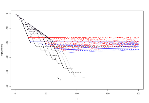
Figure 1: Plot of $\log_{10}\left|\left|D_{k}^{k+1}(i)\right|\right|_{\infty}$ ($y$-axis) for $1\leqslant k\leqslant 9$ (from left to right), and $1\leqslant i\leqslant 100$ ($x$-axis) for the pattern $\mathcal{W}={\tt GNTGNNGG}$ over the DNA alphabet $\mathcal{A}=\{{\tt A},{\tt C},{\tt G},{\tt T}\}$ (${\tt N}$ symbol meaning “any letter”) using a order $d=1$ Markov model. The curves are obtained through Algorithm 3 using recurrence relation Lemma : a) only (Red curve); b) only (Blue curve); a) and b) keeping the $D_{k}^{j}(i)$ displaying the smallest norm (Black curve). All missing values correspond to $\left|\left|D_{k}^{k+1}(i)\right|\right|_{\infty}=0$.

On Figure 1 we study empirically the convergence of $D_{k}^{k+1}(i)$ towards $\mathbf{0}$ by computing $\left|\left|D_{k}^{k+1}(i)\right|\right|_{\infty}$ for several $k$ through Algorithm 3. We consider here three way of updating $D_{k}^{j}(i)$: by using only through $D_{k}^{j-1}(i)-D_{k}^{j-1}(i-1)$ (Red curve); by using only through $TD_{k}^{j}(i-1)+QD_{k-1}^{j}(i-1)$ (Blue curve); or by taking the update which displays the smallest norm (Black curve). If these three alternative approaches give similar results when $\left|\left|D_{k}^{k+1}(i)\right|\right|_{\infty}\geqslant 10^{-15}$ differences start to appear for smaller values. The differential recurrence relation (Red curve) quickly start to accumulate machine precision residuals and results in noisy curves with a slow increasement. When using the matrix recurrence relation (Blue curve) a similar problem arise, however appearing slightly later and with far less noise. Surprisingly, the last approach which combine the two updating methods at each step benefits from a synergistic effect and displays a far better stability. A similar behaviour have been observed for a wide range of tested patterns (data not shown).

5.4 Near Gaussian approximations

Gaussian approximations for random pattern counts are widely used in the literature. We want here to push forward this idea by taking advantage of higher order moments to get near Gaussian approximations. This well known technique is described in details in Appendix B.

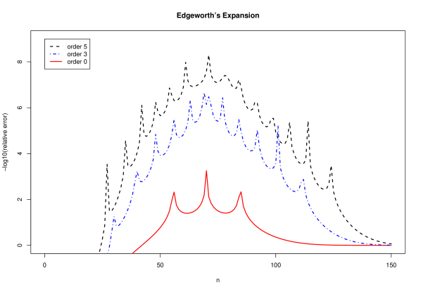
Figure 2: Relative error in decimal log scale of Edgeworth’s expansion of order $s=0$ (Red-solid), order $s=3$ (Blue-dotdashed), and order $s=5$ (Black-dashed) for Pattern ${\tt GCTGGT}$ on a order 1 homogeneous Markov model (parameter estimated on the complete genome of E. coli) of length $\ell=400\,000$.

We can see on Figure 2 the relative error (in log-scale) of several Edgeworth’s approximations for the distribution of pattern ${\tt GCTGGT}$. The solid line shows the reliability of plain Gaussian approximation (which correspond to an order $s=0$ Edgeworth’s expansion). Unsurprisingly, this approximation works better around the expectation ($\mathbb{E}[N]=70.09$ according to Table 1) providing two exact digits on the range $[54;85]$, and one exact digit on the range $[50;92]$. Beyond these limit, we get too far in the tail distribution to get reliable results. This behaviour is exactly what we expect from the central limit theory.

If we consider now order $s=3$ Edgeworth’s expansion (that uses moments up to order $k=5$) depicted with a dotdashed line on Figure 2, we see a dramatic improvement both on the accuracy of the approximation (up to 6 exact digits) and on the range of reliability (at least one exact digit on $[28;118]$). We can even get a further improvement by considering order $s=5$ expansion (dashed line) which uses moments up to order $k=7$. In both case however, the reliability of these approximations decreases dramatically when we get far enough in the tail distributions.

We observe a very similar behaviour for Pattern ${\tt AGAGAG}$ and Pattern ${\tt GGGGGG}$ and the corresponding figures are hence not shown to save space.

Thanks to this work we see that for a modest additional cost (computing moments up to order $k=5$ or $k=7$ instead of simple first and second moments), one can dramatically improve the reliability of Gaussian approximations for pattern problems.

5.5 Near Poisson approximations

A very common alternative to Gaussian approximations for random pattern counts is to turn towards Poisson approximations. These approximations are known to be quite accurate for non-overlapping patterns, but also to fail for highly self overlapping patterns for which compound Poisson approximations are known to perform better. We want here to evaluation the interest of near Poisson approximations provided by the Gram-Charlier Type B series described in Appendix C.

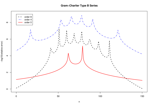
Figure 3: Relative error in decimal log scale of Gram-Charlier type B approximation of order $s=0$ (Red-solid) to order $s=4$ (Blue-dotdashed) to order $s=8$ (Black-dashed) for Pattern ${\tt GCTGGT}$ on a order 1 homogeneous Markov model (parameter estimated on the complete genome of E. coli) of length $\ell=400\,000$.

For the non-overlapping pattern ${\tt GCTGGT}$, we can see on Figure 3 that the plain Poisson approximation (order $s=0$ Gram-Charlier Type B series) gives already very good results with at least one exact digit on all the distribution, and up to 4 or 5 of them in the region close to the expectation. This interesting result is dramatically improved by the order $s=4$ approximations which gives at least 4 exact digits on all the considered range and more that 8 exact digits around the expectation. Surprisingly, the order $s=8$ approximation is less reliable than the previous one, and gives even worse results that the plain Poisson approximation in the tail distributions. This is due to the fact that the coefficients $c_{k}$ computed according to Equation (27) accumulate large terms that compensate each other. This is a typical scenario for large relative errors in floating point arithmetic. One can solve this problem either by performing computations with an arbitrary number of digits (usually slow=), or one can explicitly compute the expected relative error with the current machine-precision and renounce to use unreliable coefficients.

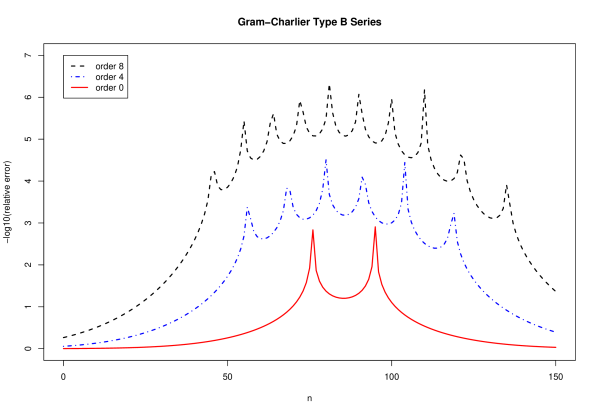
Figure 4: Relative error in decimal log scale of Gram-Charlier type B approximation of order $s=0$ (Red-solid) to order $s=4$ (Blue-dotdashed) to order $s=8$ (Black-dashed) for Pattern ${\tt AGAGAG}$ on a order 1 homogeneous Markov model (parameter estimated on the complete genome of E. coli) of length $\ell=400\,000$.

If we consider now the self-overlapping pattern ${\tt AGAGAG}$, we know from theory that Poisson approximations are not supposed to perform well. This is the reason why we observe on Figure 4 that the plain Poisson approximations only works on a very limited range the distribution (roughly on $[69;103]$). Once again however, order $s=4$ or $s=8$ Gram-Charlier expansion dramatically improve the reliability of the approximations getting up to 6 exact digits close to the expectation and at least one exact digits on a much wider range (up to $[24;150]$ for order $s=8$). One should note that in this case, the numerical issue observed for high order approximations for the previous pattern does not occur. We get a very similar result for the even more self-overlapping pattern ${\tt GGGGGG}$ and the corresponding figure is then omitted to save space.

Like with near Gaussian approximations, we see that near Poisson approximations can dramatically improve the reliability of Poisson approximations for a very modest cost (ex: computing moments up to order $k=4$ or $k=8$).

6 Conclusion

In this paper, we have derived from the explicit expression of the mgf of a pattern random count $N$, a new formula allowing to compute a arbitrary number $k$ of moments of $N$. We also have introduced three efficient algorithms to perform this computation. The first one allow the computation of pattern count moments of arbitrary order in the framework heterogeneous Markov model which is a completely new result (up to our knowledge). The second algorithm, suitable for homogeneous models and low complexity patterns, appear to have a better or similar complexity to state-of-the art known algorithms but with a far much simpler implementation. Finally, the third algorithms uses partial recursions exploiting the sparse structure of the transition matrix to provide a logarithmic complexity with the sequence length even for high complexity patterns. This very promising approach however suffers from numerical instabilities in floating point arithmetic that need to be further investigated.

One should note that our main result can be easily extended to mixed moments of several pattern counts. In order to save space, we give here such as result only for the particular case of two patterns $\mathcal{W}_{1}$ and $\mathcal{W}_{2}$ in a homogeneous model. We assume that the final states of or DFA could be partitioned into $\mathcal{F}=\mathcal{F}_{1}\cup\mathcal{F}_{2}$ such as $\mathcal{F}_{1}$ (resp. $\mathcal{F}_{2}$) count the number $N_{1}$ (resp. $N_{2}$) of occurrences of $\mathcal{W}_{1}$ (resp. $\mathcal{W}_{2}$). This is always possible by duplicating states. We consider

$$f(y_{1},y_{2})\stackrel{{\scriptstyle\text{def}}}{{=}}\sum_{n_{1},n_{2}\geqslant 0}\mathbb{P}(N_{1}=n_{1},N_{2}=n_{2})y_{1}^{n_{1}}y_{2}^{n_{2}}$$ (18)

and we then have $f(y_{1},y_{2})=\mu_{d}(P+y_{1}Q_{1}+y_{2}Q_{2})^{\ell-d}\mathbf{1}$. By introducing now $g(y_{1},y_{2})\stackrel{{\scriptstyle\text{def}}}{{=}}\mu_{d}\left(T+y_{1}Q_{1}+y_{2}Q_{2}\right)^{\ell-d}\mathbf{1}$ we get for any $k_{1},k_{2}\geqslant 0$ that:

$$\mathbb{E}\left(\frac{N_{1}!}{(N_{1}-k_{1})!}\times\frac{N_{2}!}{(N_{2}-k_{2})!}\right)=k_{1}!k_{2}![g(y_{1},y_{2})]_{y_{1}^{k_{1}}y_{2}^{k_{2}}}.$$ (19)

As an application, we have considered the distribution of DNA patterns in genomic sequences. In this particular framework, we have shown how order $k=3$ and $k=4$ moments allow to get a better description of the distribution (with quantities like skewness and excess kurtosis). We have also considered moment-based approximations namely Edgeworth’s expansion (near Gaussian approximations) and Gram-Charlier Type B series (near Poisson approximations). For both approximations, we have seen how the additional information provided by a couple of higher order moments can dramatically improve the reliability of these common approximations. As a perspective, it seems to be very promising to develop near geometric or compound Poisson distribution with Gram-Charlier Type B series.

APPENDIX

Appendix A Moments and cumulants

For any random variable $X$ and for any $k\geqslant 0$ we define the following quantities: $g_{k}\stackrel{{\scriptstyle\text{def}}}{{=}}1/k!\mathbb{E}\left[X!/(X-k)!\right]$ the coefficient of degree $k$ in the polynomial $g(y)$ defined in Section 3; $m^{\prime}_{k}\stackrel{{\scriptstyle\text{def}}}{{=}}\mathbb{E}(X^{k})$ the moment of order $k$; $m_{k}\stackrel{{\scriptstyle\text{def}}}{{=}}\mathbb{E}[(N-m^{\prime}_{1})^{k}]$ the centered moment of order $k$; and $\kappa_{k}$ the cumulant of order $k$ defined by $h(t)\stackrel{{\scriptstyle\text{def}}}{{=}}\log\mathbb{E}(e^{tN})=\sum_{k\geqslant 1}\kappa_{k}(t^{k}/k!)$. Cumulants and moments are connected through the following formula:

$$\kappa_{k}=m^{\prime}_{k}-\sum_{l=1}^{k-1}{k-1\choose l-1}\kappa_{l}m^{\prime}_{k-l}.$$ (20)

Using this formula we get: $\kappa_{1}=\mathbb{E}(X)$ and $\kappa_{2}=m_{2}=\mathbb{V}(X)$, $\kappa_{3}=m_{3}$, and $\kappa_{4}=m_{4}-3m_{2}^{2}$. The skewness $\gamma_{1}$ and excess kurtosis can be expressed from cumulants: $\gamma_{1}=\kappa_{3}/\kappa_{2}^{3/2}$ and $\gamma_{2}=\kappa_{4}/\kappa_{2}^{2}$.

Appendix B Edgeworth’s expansion

This is directly taken from [5] except the explicit order 5 expansion given in Equation (24) which is a new contribution (only order 3 explicit expansions seems to be available in the literature).

Let $X$ be a centered random variable ($\mathbb{E}[X]=0$) that admit finite moments of all orders (we denote by $\sigma^{2}$ the variance of $X$), let $\Phi$ defined by $\Phi(t)\stackrel{{\scriptstyle\text{def}}}{{=}}\mathbb{E}[e^{iX}]$ (where $i$ denote the imaginary complex number) be its caracteristic function. Let $\varphi$ be the caracteristic function of $X/\sigma$, we have $\varphi(t)=\Phi(t/\sigma)$. The definition of cumulants (see Appendix A) then allows to write the expansion:

$$\log\phi(t)=\log\Phi(t/\sigma)\sim\sum_{k=2}^{\infty}\frac{\kappa_{k}}{\sigma^{k}k!}(it)^{k}$$ (21)

then by denoting $S_{k}\stackrel{{\scriptstyle\text{def}}}{{=}}\kappa_{k}/\sigma^{2k-2}$ we get

$$\phi(t)\sim\exp\left\{\sum_{r=1}^{\infty}\frac{S_{r+2}\sigma^{r}}{(r+2)!}(it)^{r+2}\right\}.$$ (22)

The Fourier transform of expansion (22) then gives:

$$q(x)=Z(x)\left(1+\sum_{s=1}^{\infty}\sigma^{s}\times\left\{\sum_{\{k_{m}\}_{s}}H_{s+2r}(x)\prod_{m=1}^{s}\frac{1}{k_{m}!}\left(\frac{S_{m+2}}{(m+2)!}\right)^{k_{m}}\right\}\right)$$ (23)

where $q(x)\stackrel{{\scriptstyle\text{def}}}{{=}}\sigma p(\sigma x)$ is the probability distribution function (pdf) of $X/\sigma$ ($p(x)$ being the pdf of $X$), where $Z(x)=\exp(-x^{2}/2)/\sqrt{2\pi}$ is the pdf of a standard Gaussian variable, where $\{k_{m}\}_{s}$ is the set of all non-negative integer solution of the Diophantine equation $k_{1}+2k_{2}+\ldots+sk_{s}=s$, $r=k_{1}+k_{2}+\ldots+k_{s}$, and where $H_{k}(x)$ are the Hermite polynomials defined recursively by $H_{0}(x)\stackrel{{\scriptstyle\text{def}}}{{=}}1$ and $H_{k}(x)\stackrel{{\scriptstyle\text{def}}}{{=}}xH_{k-1}(x)-H_{k-1}^{\prime}(x)$ for all $k\geqslant 1$.

Here are the sets of $\{k_{m}\}_{s}$ for $1\leqslant s\leqslant 5$: $\{k_{m}\}_{1}=\{1\}$, $\{k_{m}\}_{2}=\{20,01\}$, $\{k_{m}\}_{3}=\{300,110,001\}$, $\{k_{m}\}_{4}=\{4000,2100,0200,1010,0001\}$, and $\{k_{m}\}_{5}=\{50000,31000,12000,$ $20100,01100,10010,00001\}$, and here is the explicit expression of (23) up to order $s=5$ (such an explicit expression can be found up to $s=3$ in [4]):

$$\frac{q(x)}{Z(x)}\simeq 1+\sigma\left\{H_{3}(x)\frac{S_{3}}{3!}\right\}\\ +\sigma^{2}\left\{H_{4}(x)\frac{S_{4}}{4!}+H_{6}(x)\frac{S_{3}^{2}}{2!3!^{2}}\right\}+\sigma^{3}\left\{H_{5}(x)\frac{S_{5}}{5!}+H_{7}(x)\frac{S_{3}S_{4}}{3!4!}+H_{9}(x)\frac{S_{3}^{3}}{3!^{4}}\right\}\\ +\sigma^{4}\left\{H_{6}(x)\frac{S_{6}}{6!}+H_{8}(x)\left(\frac{S_{3}S_{5}}{3!5!}+\frac{S_{4}^{2}}{2!4!^{2}}\right)+H_{10}(x)\frac{S_{3}^{2}S_{4}}{2!3!^{2}4!}+H_{12}(x)\frac{S_{3}^{4}}{4!3!^{4}}\right\}\\ +\sigma^{5}\left\{H_{7}(x)\frac{S_{7}}{7!}+H_{9}(x)\left(\frac{S_{4}S_{5}}{4!5!}+\frac{S_{3}S_{6}}{3!6!}\right)+H_{11}(x)\left(\frac{S_{3}^{2}S_{5}}{2!3!^{2}5!}+\frac{S_{3}S_{4}^{2}}{2!3!4!^{2}}\right)\right.\\ \left.+H_{13}(x)\frac{S_{3}^{3}S_{4}}{3!^{4}4!}+H_{15}(x)\frac{S_{3}^{5}}{5!3!^{5}}\right\}$$ (24)

Appendix C Gram-Charlier type B serie for near Poisson distribution

This is initially taken from [2] but we derive new recurrence relation that are more adapted to a modern computational framework than the explicit (and sometimes erroneous) formulas given in the original article.

Let $\psi(i)\stackrel{{\scriptstyle\text{def}}}{{=}}e^{-\lambda}\lambda^{i}/i!$ be the pdf of a Poisson distribution of parameter $\lambda$, and let $\Delta$ be the differential operator defined by $\Delta\psi(i)\stackrel{{\scriptstyle\text{def}}}{{=}}\psi(i)-\psi(i-1)$. Our objective is to approximate the pdf $F$ of a discrete non-negative random variable $X$ with

$$F(i)\simeq\sum_{j=0}^{s}c_{j}\Delta^{j}\psi(i)$$ (25)

In order to do so we use a moment method and find a solution $(c_{0},c_{1},\ldots,c_{s})$ of $\sum_{j=0}^{s}c_{j}P_{k}^{j}(\lambda)=\mathbb{E}[X^{k}]$ for all $0\leqslant k\leqslant s$ with $P_{k}^{j}(\lambda)\stackrel{{\scriptstyle\text{def}}}{{=}}\sum_{i\geqslant 0}i^{k}\Delta^{j}\psi(i)$ for all $j,k\geqslant 0$.

It is clear that we have $P_{0}^{0}(\lambda)=1$, and we have the following recurrence relation for all $k,j\geqslant 0$:

$$P_{k+1}^{0}(\lambda)=\lambda\left[P_{k}^{0}(\lambda)+\frac{dP_{k}^{0}}{d\lambda}(\lambda)\right]\quad\text{and}\quad P_{k}^{j+1}(\lambda)=-\frac{dP_{k}^{j}}{d\lambda}(\lambda).$$ (26)

We hence get that $c_{0}=1$ and we derive the following recurrent relation for $k\geqslant 1$:

$$c_{k}=\frac{1}{P_{k}^{k}(\lambda)}\left(\mathbb{E}[X^{k}]-\sum_{j=0}^{k-1}c_{j}P_{k}^{j}(\lambda)\right).$$

Please note that $P_{k}^{k}(\lambda)$ is always a scalar. If we now denote by $g_{k}\stackrel{{\scriptstyle\text{def}}}{{=}}1/k!\mathbb{E}\left[X!/(X-k)!\right]$ the we can show by recurrence for all $k\geqslant 1$ that we finally have:

$$c_{k}=-\frac{(k-1)}{k!}g_{1}^{k}+\sum_{j=2}^{k}(-1)^{j}\frac{g_{1}^{k-j}g_{j}}{(k-j)!}$$ (27)

Here are the explicit first $5$ terms of this formula:

$$c_{2}=g_{2}-\frac{g_{1}^{2}}{2}\quad c_{3}=-g_{3}+g_{1}g_{2}-\frac{g_{1}^{3}}{3}\quad c_{4}=g_{4}-g_{1}g_{3}+\frac{g_{1}^{2}g_{2}}{2}-\frac{g_{1}^{4}}{8}$$

$$c_{5}=-g_{5}+g_{1}g_{4}-\frac{g_{1}^{2}g_{3}}{2}+\frac{g_{1}^{3}g_{2}}{6}-\frac{g_{1}^{5}}{30}\quad c_{6}=g_{6}-g_{1}g_{5}+\frac{g_{1}^{2}g_{4}}{2}-\frac{g_{1}^{3}g_{3}}{6}+\frac{g_{1}^{4}g_{2}}{24}-\frac{g_{1}^{6}}{144}.$$

References

• [1] Antzoulakos, D.ย L. (2001). Waiting times for patterns in a sequence of multistate trials. J. Appl. Prob. 38, 508โ€“518.
• [2] Aroian, L.ย A. (1937). The Type B Gram-Charlier Series. The Ann. of Math. Stat. 8, 183โ€“192.
• [3] Beaudoing, E., Freier, S., Wyatt, J., Claverie, J.-M. and Gautheret, D. (2000). Patterns of variant polyadenylation signal usage in human genes. Genome Res. 10, 1001โ€“1010.
• [4] Bernardeau, F. and Kofman, L. (1995). Properties of the cosmological density distribution function. Astrophys. J. 443, 479โ€“498.
• [5] Blinnikov, S. and Moessner, R. (1998). Expansions for nearly Gaussian distributions. Astron. Astrophys. Suppl. Ser. 130, 193โ€“205.
• [6] Boeva, V., Clement, J., Regnier, M., Roytberg, M. and Makeev, V. (2007). Exact p-value calculation for heterotypic clusters of regulatory motifs and its application in computational annotation of cis-regulatory modules. Algorithms for Molecular Biology 2, 13.
• [7] Boeva, V., Clรฉment, J., Rรฉgnier, M. and Vandenbogaert, M. (2005). Assessing the significance of sets of words. In Combinatorial Pattern Matching 05, Lecture Notes in Computer Science, vol. 3537. Springer-Verlag.
• [8] Brazma, A., Jonassen, I., Vilo, J. and Ukkonen, E. (1998). Predicting gene regulatory elements in silico on a genomic scale. Genome Res. 8, 1202โ€“1215.
• [9] Chang, Y.-M. (2005). Distribution of waiting time until the rth occurrence of a compound pattern. Statistics and Probability Letters 75, 29โ€“38.
• [10] Cowan (1991). Expected frequencies of dna patterns using whittleโ€™s formula. J. Appl. Prob. 28, 886โ€“892.
• [11] Crochemore, M. and Stefanov, V. (2003). Waiting time and complexity for matching patterns with automata. Info. Proc. Letters 87, 119โ€“125.
• [12] Denise, A., Rรฉgnier, M. and Vandenbogaert, M. (2001). Assessing the statistical significance of overrepresented oligonucleotides. Lecture Notes in Computer Science 2149, 85โ€“97.
• [13] Elย Karoui, M., Biaudet, V., Schbath, S. and Gruss, A. (1999). Characteristics of chi distribution on different bacterial genomes. Res. Microbiol. 150, 579โ€“587.
• [14] Erhardsson, T. (2000). Compound Poisson approximation for counts of rare patterns in Markov chains and extreme sojourns in birth-death chains. Ann. Appl. Probab. 10, 573โ€“591.
• [15] Frith, M.ย C., Spouge, J.ย L., Hansen, U. and Weng, Z. (2002). Statistical significance of clusters of motifs represented by position specific scoring matrices in nucleotide sequences. Nucl. Acids. Res. 30, 3214โ€“3224.
• [16] Fu, J.ย C. (1996). Distribution theory of runs and patterns associated with a sequence of multi-state trials. Statistica Sinica 6, 957โ€“974.
• [17] Geske, M.ย X., Godbole, A.ย P., Schaffner, A.ย A., Skrolnick, A.ย M. and Wallstrom, G.ย L. (1995). Compound poisson approximations for word patterns under markovian hypotheses. J. Appl. Probab. 32, 877โ€“892.
• [18] Godbole, A.ย P. (1991). Poissons approximations for runs and patterns of rare events. Adv. Appl. Prob. 23,.
• [19] Hampson, S., Kibler, D. and Baldi, P. (2002). Distribution patterns of over-represented k-mers in non-coding yeast DNA. Bioinformatics 18, 513โ€“528.
• [20] Karlin, S., Burge, C. and Campbell, A. (1992). Statistical analyses of counts and distributions of restriction sites in DNA sequences. Nucl. Acids. Res. 20, 1363โ€“1370.
• [21] Kleffe, J. and Borodovski, M. (1997). First and second moment of counts of words in random texts generated by markov chains. Bioinformatics 8, 433โ€“441.
• [22] Leonardo Mariรฑo-Ramรญrez, John L.ย Spouge, G. C.ย K. and Landsman, D. (2004). Statistical analysis of over-represented words in human promoter sequences. Nuc. Acids Res. 32, 949โ€“958.
• [23] Lladser, M.ย E. (2007). Mininal markov chain embeddings of pattern problems. In Information Theory and Applications Workshop. pp.ย 251โ€“255.
• [24] Lothaire, M., Ed. (2005). Applied Combinatorics on Words. Cambridge University Press, Cambridge.
• [25] Nicodรจme, P., Salvy, B. and Flajolet, P. (2002). Motif statistics. Theoretical Com. Sci. 287, 593โ€“617.
• [26] Nuel, G. (2004). Ld-spatt: Large deviations statistics for patterns on markov chains. J. Comp. Biol. 11, 1023โ€“1033.
• [27] Nuel, G. (2006). Effective p-value computations using Finite Markov Chain Imbedding (FMCI): application to local score and to pattern statistics. Algorithms for Molecular Biology 1, 5.
• [28] Nuel, G. (2006). Numerical solutions for patterns statistics on markov chains. Stat. App. in Genet. and Mol. Biol. 5, 26.
• [29] Nuel, G. (2008). Pattern Markov chains: optimal Markov chain embedding through deterministic finite automata. J. of Applied Prob. 45, 226โ€“243.
• [30] Pevzner, P., Borodovski, M. and Mironov, A. (1989). Linguistic of nucleotide sequences: The significance of deviation from mean statistical characteristics and prediction of frequencies of occurrence of words. J. Biomol. Struct. Dyn. 6, 1013โ€“1026.
• [31] Prum, B., Rodolphe, F. and deย Turckheim, E. (1995). Finding words with unexpected frequencies in dna sequences. J. R. Statist. Soc. B 11, 190โ€“192.
• [32] Reignier, M. (2000). A unified approach to word occurrences probabilities. Discrete Applied Mathematics 104, 259โ€“280.
• [33] Reinert, G. and Schbath, S. (1999). Compound poisson and poisson process approximations for occurrences of multiple words in markov chains. J. of Comp. Biol. 5, 223โ€“254.
• [34] Ribeca, P. and Raineri, E. (2008). Faster exact Markovian probability functions for motif occurrences: a DFA-only approach. Bioinformatics 24, 2839โ€“2848.
• [35] Stefanov, V. and Pakes, A.ย G. (1997). Explicit distributional results in pattern formation. Ann. Appl. Probab. 7, 666โ€“678.
• [36] Stefanov, V.ย T. and Szpankowski, W. (2007). Waiting Time Distributions for Pattern Occurrence in a Constrained Sequence. Discrete Mathematics and Theoretical Computer Science 9, 305โ€“320.
• [37] van Helden, J., Andrรฉ, B. and Collado-Vides, J. (1998). Extracting regulatory sites from the upstream region of yeast genes by computational analysis of oligonucleotide frequencies. J. Mol. Biol. 281, 827โ€“842.