Asymptotic Entanglement Dynamics Phase Diagrams for Two Electromagnetic Field Modes in a Cavity

Abstract

We investigate theoretically an open dynamics for two modes of electromagnetic field inside a microwave cavity. The dynamics is Markovian and determined by two types of reservoirs: the “natural” reservoirs due to dissipation and temperature of the cavity, and an engineered one, provided by a stream of atoms passing trough the cavity, as devised by Pielawa et al. [Phys. Rev. Lett. 98, 240401 (2007)]. We found that, depending on the reservoir parameters, the system can have distinct “phases” for the asymptotic entanglement dynamics: it can disentangle at finite time or it can have persistent entanglement for large times, with the transition between them characterized by the possibility of asymptotical disentanglement. Incidentally, we also discuss the effects of dissipation on the scheme proposed in the above reference for generation of entangled states.

I Introduction

In recent years, the problem of entanglement dynamics has gained the attention of the quantum-information community esd . Despite the fact that some recent results contradict the intuition that “the more entangled the better” Bacon-Phys , to protect entanglement is yet an important concern when one wants to make quantum computers. The first works on the “fate” of entanglement on an open system focused on two or more qubit systems. Curious names such as entanglement sudden death have appeared, first by the recognition of the possibility of entanglement between two qubits to vanish in finite time, although coherences only decay exponentially. Similar phenomena also happen for continuous variables (CV) systems esdcv . A general geometrical picture has already been offered showing that the long term behavior of entanglement depends essentially on the set of asymptotic states GeoSudDeath .

In a series of papers, Paz and Roncaglia studied some phase diagrams for the asymptotic behavior of entanglement on two-mode Gaussian states (GS) exposed to a common thermal environment PR . In particular, they built them in terms of squeezing and temperature for two harmonic oscillators. For the resonant case, they found three very distinct possible fates: entanglement can suffer from sudden death, can enter in a perpetual cycle of death and birth, or can be persistent. From a different perspective, Pielawa et al. made a proposal of how to use an engineered reservoir to create two-mode Gaussian entangled states in cavity quantum electrodynamics (CQED) davidov .

In this paper we make a threefold study: we generalize the studies from Paz and Roncaglia, by constructing phase diagrams in terms of different variables, for systems subjected to not only natural reservoirs, but also this engineered one; we show how those phase diagrams can be experimentally obtained; and incidentally we study the robustness, against thermal noise, of the engineered reservoir strategy for generating two-mode entangled states.

The next section is devoted to reviewing some basics about two-mode GS and the proposal for generating entangled ones in CQED davidov . Section III is the central part of our study, where the entanglement dynamics of two modes subjected to thermal noise and the engineered reservoir is discussed. The experimental proposal is focused in Sec. IV, followed by the study of the robustness of the method suggested in Ref. davidov . Discussion and concluding remarks close the paper.

II Preliminaries

Here we will review some necessary definitions and tools in the theory of entanglement of GS and also the scheme to implement the engineered reservoir.

II.1 Entanglement in Gaussian States

Many of the protocols and techniques from the entanglement theory of finite dimensional systems can be adapted to CV systems, usually restricted to the set of GS. For instance, the protocols of teleportation teleporte ; teleportecv and quantum key distribution qkd ; qkdcv have their analogs for CV systems (and may be more robust experimentally expqks ); the Peres-Horodecki peres ; pereshorodecki separability criteria can be applied, and is also necessary and sufficient for two-mode GS simon ; and entanglement quantifiers such as negativity neg , logarithmic negativity logneg , and entanglement of formation enform can be computed within the formalism of symplectic geometry negcv ; enformcv ; adesso .

GS are defined as those states whose Wigner characteristic function is Gaussian, so they are completely described by its first and second statistical momenta. First momenta, mean values, can be locally changed by redefining the mode operators, so all entanglement information is given by second momenta. Choosing only two modes, with destruction operators $\hat{a}_{j}=(\hat{x}_{i}+i\hat{p}_{i})/\sqrt{2}$, $i=1,2$, and corresponding quadrature amplitudes $\hat{x}_{i},\hat{p}_{i}$, the Wigner characteristic function of a state $\hat{\rho}$ is given by $\chi(z_{1},z_{2})=\text{Tr}[\hat{\rho}\exp{(z_{1}\hat{a}_{1}-z_{1}^{*}\hat{a}_{1}^{\dagger}+z_{2}\hat{a}_{2}-z_{2}^{*}\hat{a}_{2}^{\dagger})}]$, where $z_{i}$ are complex numbers. The state second momenta, on the other hand, are well grouped under its covariance matrix (CM):

$$V_{\hat{\rho}}=\left(\begin{array}[]{cccc}n_{1}+\frac{1}{2}&m_{1}&m_{s}&m_{c}\\ m_{1}^{*}&n_{1}+\frac{1}{2}&m_{c}^{*}&m_{s}^{*}\\ m_{s}^{*}&m_{c}&n_{2}+\frac{1}{2}&m_{2}\\ m_{c}^{*}&m_{s}&m_{2}^{*}&n_{2}+\frac{1}{2}\end{array}\right),$$ (5)

where $n_{j}=\langle\hat{a}^{\dagger}_{j}\hat{a}_{j}\rangle$, $m_{j}=-\langle\hat{a}_{j}^{2}\rangle$, $m_{s}=-\langle\hat{a}_{1}\hat{a}_{2}^{\dagger}\rangle$, $m_{c}=\langle\hat{a}_{1}\hat{a}_{2}\rangle$, and $\langle\hat{\xi}\rangle$ denotes the quantum expectation value $\text{Tr}\hat{\xi}\hat{\rho}$ of an observable $\hat{\xi}$. The state is Gaussian (with null first momenta) if and only if $\chi(z_{1},z_{2})=\exp{(-\frac{1}{2}\textbf{z}^{\dagger}V_{\hat{\rho}}\textbf{z})}$, where $\textbf{z}^{t}=(z_{1},z_{1}^{*},z_{2},z_{2}^{*})$.

We can write the CV as a block matrix, as follows:

$$V_{\hat{\rho}}=\left(\begin{array}[]{cc}V_{1}&C\\ C^{\dagger}&V_{2}\end{array}\right),$$ (8)

where $V_{i}$ is a $2\times 2$ matrix related to the mode $i$, and $C$ is a $2\times 2$ matrix that gives the correlations (both quantum and classical) between the modes. One should note that to represent a quantum state, a CM should also obey the generalized Robertson-Schrödinger uncertainty relations adesso . A CM not obeying such relations is called nonphysical.

Simon simon has shown that, as for two qubits, the Peres-Horodecki criterion pereshorodecki is decisive for entanglement of two-mode GS, and it can be given in terms of the quantity:

$$S\left(V_{\hat{\rho}}\right)=I_{1}I_{2}+(1/4-|I_{3}|)^{2}-I_{4}-1/4(I_{1}+I_{2}),$$ (9a)

where $$I_{1,2}=\det V_{1,2} I_{3}=\det C I_{4}=\operatorname{tr}\left[V_{1}ZCZV_{2}ZC^{\dagger}Z\right] Z=\text{diag}\{1,-1\}$$, , and are invariants under local unitary operations, with . A GS is separable if and only if

$$S\left(V_{\hat{\rho}}\right)\geq 0,$$ (9b)

the so-called Simon criterion.

Entanglement in two-mode systems reminds Einstein-Podolsky-Rosen (EPR) discussion on completeness of quantum mechanics EPR . Indeed, entanglement in this system is closely related to squeezing in “EPR-like quadratures. Given any local operators $\hat{Q}_{i},\hat{P}_{i}$ satisfying the commutation relations $[\hat{Q}_{i},\hat{P}_{i}]=i\hbar$, for any arbitrary real number $a\neq 0$ one can define the pair of EPR-like operators $\hat{u}=|a|\hat{Q}_{1}+\frac{1}{a}\hat{Q}_{2}$, $\hat{v}=|a|\hat{P}_{1}-\frac{1}{a}\hat{P}_{2}$. Duan et al. DGCZ have shown that if a state is separable, then $\langle\Delta\hat{u}^{2}\rangle+\langle\Delta\hat{v}^{2}\rangle\geq a^{2}+1/a^{2}$. Hence, if this pair of EPR operators is squeezed enough, i.e., if the sum of their variances violates the inequality, the state is entangled for sure.

For GS, this criterion is necessary and sufficient to decide separability, which we shall call the Duan-Giedke-Cirac-Zoller (DGCZ) criterion. This is done representing the CM in a standard form, through local Gaussian operations, so that the validity of the above inequality applied to the matrix in this form, with $a$ determined by its coefficients, implies that the state is separable. Restricting further to the set of symmetric states, it is sufficient to consider $|a|=1$, and the procedure amounts to finding, through local rotations and squeezing of the quadratures $\hat{x}_{i},\hat{p}_{i}$, which pair of EPR-like operators have the least value for the sum of their variances.

We shall deal mostly with symmetric GS (i.e. $I_{1}=I_{2}$), and for these we shall use the Entanglement of Formation as an entanglement quantifier, which has an explicit formula rigol

$$E_{F}(\rho)=f(2\sqrt{I_{1}+|I_{3}|-\sqrt{I_{4}+2I_{1}|I_{3}|}})$$ (10)

where $f(x)=c_{+}(x)\log_{2}c_{+}(x)-c_{-}(x)\log_{2}c_{-}(x)$, with $c_{\pm}(x)=\frac{1}{4}(x^{-1/2}\pm x^{1/2})^{2}$.

II.2 Two-mode entanglement from engineered reservoir

To make the context clear, we now review the scheme for constructing the common squeezing reservoir between the modes davidov . We also take the opportunity to introduce notation and to explicit the dependence of the final master equation on the several parameters of the setting.

Consider two modes of electromagnetic field of a high quality microwave cavity, with frequencies $\omega_{1}$ and $\omega_{2}$. As before, $\hat{a}_{i}$ denotes the annihilation operator for mode $i$. The engineered reservoir is provided by a stream of atoms passing through the cavity. The atoms are first prepared in a specific superposition of two Rydberg states denoted $\left|g\right\rangle$ and $\left|e\right\rangle$, then they pass through the cavity, where they can interact with the two nondegenerate modes, while a classical field (injected externally in the setup of open cavities) saturates the dipole transition, pumping the two modes. The Hamiltonian that describes such setup is:

$$\hat{H} = \hbar\omega_{0}\hat{\sigma}^{+}\hat{\sigma}^{-}+\hbar\Omega(e^{-i\omega_{L}t}\hat{\sigma}^{+}+e^{i\omega_{L}t}\hat{\sigma}^{-})$$ (11)

$$+\sum_{i}[\hbar\omega_{i}\hat{a}_{i}^{\dagger}\hat{a}_{i}+\hbar g_{i}(\hat{a}_{i}\hat{\sigma}^{+}+\hat{a}_{i}^{\dagger}\hat{\sigma}^{-})],$$

where $\omega_{0}$ is the transition frequency between the atomic levels, $g_{i}$ are the coupling constants between the atom and the modes, $\hat{\sigma}^{+}$ and $\hat{\sigma}^{-}$ are the atomic ladder operators. The coupling with the external classical field, with strength $\Omega$, is described by the time dependent part. For future reference, we set $\Delta=\omega_{L}-\omega_{0}$, the detuning between the classical field and the atomic level.

The authors explore different approximations and mode redefinitions. Here we will be concerned with the regime when (i) the atomic coupling with the classical field is much stronger than with the cavity modes: $\left|\Omega\right|\gg\left|g_{i}\right|$; (ii) defining $d=\sqrt{\Delta^{2}+4\Omega^{2}}$, and choosing $\omega_{L}$ obeying $\omega_{L}-\omega_{1}=\omega_{2}-\omega_{L}=d$, with the condition $g=g_{1}=g_{2}$. Under this regime the interaction Hamiltonian can be approximated by:

$$\hat{H}_{int} \simeq -\hbar\Omega_{b}(\hat{b}_{1}\hat{\pi}^{-}+\hat{b}_{1}^{\dagger}\hat{\pi}^{+}),\text{~{}~{}~{}~{}~{} if $\Delta>0$},$$ (12a)

$$\hat{H}_{int} \simeq \hbar\Omega_{b}(\hat{b}_{2}^{\dagger}\hat{\pi}^{-}+\hat{b}_{2}\hat{\pi}^{+}),\text{~{}~{}~{}~{}~{}~{}~{} if $\Delta<0$},$$ (12b)

where $\hat{\pi}^{+}$ and $\hat{\pi}^{-}$ are ladder operators for semiclassical dressed states $\left|+\right\rangle=\sin\theta\left|g\right\rangle+\cos\theta\left|e\right\rangle$ and $\left|-\right\rangle=\cos\theta\left|g\right\rangle-\sin\theta\left|e\right\rangle$, with $\tan\theta=2\Omega/(d-\Delta)$, $\Omega_{b}$ is related to the coupling constant between the atoms and the cavity modes, $\Omega_{b}=g\sqrt{(1-\mu)/(1+\mu)}$, where $\mu=\tan^{2}\theta$ [$\mu=(\tan\theta)^{-2}$] if $|\tan\theta|<1$ [$|\tan\theta|>1$], i.e., $\mu$ is determined by the classical field parameters. The new modes are $\hat{b}_{1(2)}=\hat{S}^{\dagger}(r_{\mu})\hat{a}_{1(2)}\hat{S}(r_{\mu})=\cosh{|r_{\mu}|}a_{1(2)}-\frac{r_{\mu}}{|r_{\mu}|}\sinh{|r_{\mu}|}a^{\dagger}_{2(1)}$ defined by the well-known two-mode squeezing operator: $\hat{S}(r_{\mu})=\exp(r_{\mu}^{*}\hat{a}_{1}\hat{a}_{2}-r_{\mu}\hat{a}_{1}^{\dagger}\hat{a}_{2}^{\dagger})$, and $r_{\mu}$ is the squeezing parameter $r_{\mu}=\text{arctanh}\mu$.

If after the interaction time the atoms are ignored, the Hamiltonian of Eq. (11) implies an open system effective dynamics for the field modes. Eqs. (12) show that for $\Delta>0$ ($\Delta<0$), the interaction reduces to a (anti-) Jaynes-Cummings between the classically dressed atom and mode $\hat{b}_{1(2)}$. For $\Delta>0$ ($\Delta<0$), one simulates null temperature dissipation in mode $\hat{b}_{1(2)}$ if one prepares atoms in the state $\left|+\right\rangle$ ($\left|-\right\rangle$) and allow interaction for times, $\tau$, obeying $\Omega_{b}\tau\ll 1$. We shall call these type 1 (2) atoms. If a stream of type $j$ atoms passes trough the cavity, one at a time, the field dynamics will be Markovian, given by a differential equation in Lindblad form lindblad :

$$\frac{d\hat{\rho}}{dt}=\mathcal{D}_{j,Eng}(\hat{\rho}),$$ (13a)

where the effective engineered dissipator is given by morigi

$$\mathcal{D}_{j,Eng}(\hat{\rho})=2\kappa_{j}(2\hat{b}_{j}\hat{\rho}\hat{b}_{j}^{\dagger}-\hat{b}_{j}^{\dagger}\hat{b}_{j}\hat{\rho}-\hat{\rho}\hat{b}_{j}^{\dagger}\hat{b}_{j}),$$ (13b)

while $$\kappa_{j}=(r_{at,j}\Omega_{b}^{2}\tau^{2})/4 r_{at,j}$$ with the atomic preparation rate.

We note that, at first sight, the large frequency separation between the modes would forbid, in the regime considered here, the presence of combined terms between the modes, such as $a_{1}a_{2}^{\dagger}$ in the master equation, since they are fast oscillating compared to the total time scale of the experiment and even the interaction time of each atom [which is essential, in order to use the approximated Hamiltonian (12)]. Though, the crucial point is that the terms $a_{1}^{(\dagger)}a_{2}^{(\dagger)}$, the only combined ones present in the master equation, do not oscillate in the laser reference frame. We will come back to this point later when discussing the state evolution.

III Entanglement Dynamics under Engineered and Thermal Reservoirs

If a random source defines together the type of the atom and the suitable DC electrical field in the cavity, the dissipator for the engineered reservoir will acquire the form:

$$\mathcal{D}_{Eng}(\hat{\rho})=\mathcal{D}_{1,Eng}(\hat{\rho})+\mathcal{D}_{2,Eng}(\hat{\rho}),$$ (14)

with $\kappa_{j}=(r_{at,j}\Omega_{b}^{2}\tau^{2})/4$, $r_{at,j}$ being the type $j$ atoms flux.

The entanglement behavior will get richer when considered together with the natural dissipation and thermal noise on the modes, effects that, in usual experiments with microwave cavities, can be well described by a Lindblad equation with dissipator $\mathcal{D}_{Nat}$ given by:

$$\mathcal{D}_{Nat}(\hat{\rho}) = \sum_{i}\lambda_{i}(n_{T_{i}}+1)(2\hat{a}_{i}\hat{\rho}\hat{a}_{i}^{\dagger}-\hat{a}_{i}^{\dagger}\hat{a}_{i}\hat{\rho}-\hat{\rho}\hat{a}_{i}^{\dagger}\hat{a}_{i})$$

$$+\lambda_{i}n_{T_{i}}(2\hat{a}_{i}^{\dagger}\hat{\rho}\hat{a}_{i}-\hat{a}_{i}\hat{a}_{i}^{\dagger}\hat{\rho}-\hat{\rho}\hat{a}_{i}\hat{a}_{i}^{\dagger}),$$ (15)

where $n_{T_{i}}$ denotes the number of thermal photons and $\lambda_{i}$ the decay rate for mode $i$. Since the number of thermal photons is approximately the same for both modes if $\left|\omega_{1}-\omega_{2}\right|\ll\omega_{i}$, we shall assume from now on $n_{T_{i}}=n_{T}$.

At last, the full dynamics of the system will be described by the Lindblad equation:

$$\frac{d\hat{\rho}}{dt}=\mathcal{D}_{Nat}(\hat{\rho})+\mathcal{D}_{Eng}(\hat{\rho}),$$ (16)

with the dissipator given by Eqs. (14) and (III).

In an experimental setting one should actually consider the evolution in the laser reference frame. In this case, fast oscillations (with frequencies of the order $d$) between the modes will take place. As a consequence, in the course-grained scale necessary for the approximations to be valid, some coherences of the density matrix will vanish, making the theoretical analysis more complicated. Nevertheless, the above equation will still be valid for some initial states, i.e., they are not affected by these oscillations. Hence, in the rest of this section we shall explore the theoretical properties of Eq. (16), considering several initial states, but later, in the experimental proposal, we must guarantee the use of such robust states against this coarse-graining effect.

III.1 Symmetric engineered reservoir

Now we pass to the study of entanglement dynamics under Eq. (16). Given the specific form of the dissipators, Gaussianity is preserved, so we are safe to restrict ourselves to GS. Let us suppose first that both types of atoms enter in the cavity with equal probability, so that $\kappa_{1}=\kappa_{2}=\kappa$, and also, for the sake of simplicity, that $\lambda_{1}=\lambda_{2}=\lambda$. The equations of motion for the second momenta in this case become:

$$\dot{n_{j}} = -2(\kappa+\lambda)n_{j}+2\kappa|B|^{2}+2\lambda n_{T},$$ (17a)

$$\dot{m_{j}} = -2(\kappa+\lambda)m_{j},$$ (17b)

$$\dot{m_{c}} = -2(\kappa+\lambda)m_{c}+2\kappa AB^{*},$$ (17c)

$$\dot{m_{s}} = -2(\kappa+\lambda)m_{s},$$ (17d)

with $A=\cosh(r)$, $B=e^{i\phi}\sinh(r)$, where $r$ is the squeezing parameter and $\phi$ the squeezing angle in the definition of modes $\hat{b}_{j}$ ($r_{\mu}=re^{i\phi}$). This gives a relaxing dynamics with the asymptotic CM:

$$V_{\hat{\rho}_{f}}=\left(\begin{array}[]{cccc}n_{1,f}+\frac{1}{2}&0&0&m_{c,f}\\ 0&n_{1,f}+\frac{1}{2}&m_{c,f}^{*}&0\\ 0&m_{c,f}&n_{2,f}+\frac{1}{2}&0\\ m_{c,f}^{*}&0&0&n_{2,f}+\frac{1}{2}\end{array}\right),$$ (22)

where $n_{1,f}=n_{2,f}=\frac{|B|^{2}+n_{T}R}{1+R}$, $m_{c,f}=\frac{AB^{*}}{1+R}$, and the ratio $R=\lambda/\kappa$ was introduced.

Simon criterion can now be applied to determine whether such CM represents entangled or separable states. In the same reasoning as in Ref. GeoSudDeath , $S\left(V_{\rho_{f}}\right)>0$ implies a deep separable asymptotic state, i.e., a state belonging to the interior of the separable states set. This can be seen noting that $S$ is a continuous function, so there must exist a “ball” of GS around the asymptotic one such that $S$ is strictly positive, that is, a ball of separable GS. Hence, this translates dynamically as sudden death of entanglement (SDE), because we can say for sure that, for every initial GS, there will be a time $T$ such that the entanglement will be zero for $t>T$. In principle, though, it could undergo cycles before it vanishes for good, or an initially separable state can acquire some entanglement and (necessarily) lose it after some time. These “non-asymptotic” behaviors will be discussed in more detail on Sec. III.2.

On the other hand, states satisfying $S\left(V_{\rho_{f}}\right)<0$ represent a situation of (asymptotic) persistent entanglement (PE). Note that entanglement can be created by the common reservoir, since this is exactly the idea of the Ref. davidov proposal. But again, the intermediate dynamics can exhibit richer features; for instance, an initially entangled state can lose all entanglement at finite time but (necessarily) recover it at later time, as will be exemplified at Sec. III.2.

The exceptional situation is given by $S\left(V_{\rho_{f}}\right)=0$, when each initially entangled state can show one of two fates: sudden death of entanglement or asymptotic death of entanglement, depending on the initial state. Contrary to the former two situations, this one requires the knowledge of the whole dynamics in order to determine which fate will occur.

The situation here studied allows only one asymptotic state for each set of fixed parameters, that is why one can not see infinite cycles of birth and death as in Ref. PR , which would appear for dynamics with asymptotic periodic orbits, instead of asymptotic states.

In Fig. 1, we plot the regions in the parameter space $R\times n_{T}$ where the asymptotic state is separable or entangled, defining the fate of entanglement. The boundary curve separating the two regions in the diagram has the simple form:

$$n_{T}=\frac{e^{2r}-1}{2R}.$$ (23)

The physical interpretation is simple and meaningful. Given the engineered reservoir, for any given positive coupling ratio, $R$, there is a positive temperature, $n_{T}$, obeying (23) such that below this temperature, the asymptotic state is entangled, due to the common reservoir, while for temperatures above that critical value, the asymptotic state is separable, when (local) thermal noise prevails.

For any set of reservoir parameters, we applied the method of Duan, Giedke, Cirac, and Zoller DGCZ and found the EPR-like operators with least sum of variances, which gives $\hat{X}_{1,\phi}-\hat{X}_{2,\phi}$ and $\hat{P}_{1,\phi}+\hat{P}_{2,\phi}$, where $(\hat{X}_{i,\phi},\hat{P}_{i,\phi})^{T}=\mathcal{R}_{2\phi}(\hat{x}_{i},\hat{p}_{i})^{T}$, $\mathcal{R}_{2\phi}$ is the matrix representing a rotation in the plane trough an angle $2\phi$, $\phi$ being the squeezing angle defined by the reservoir. This is expected, since the engineered reservoir tries to lead the initial state to a usual two-mode squeezed state, known to be squeezed in these quadratures. The natural reservoir, on the other hand, enlarges their spreading. So the final decision of whether the asymptotic state will be separable or entangled will depend on this competition between the reservoirs: one trying to squeeze the collective quadratures, the other trying to spread them.

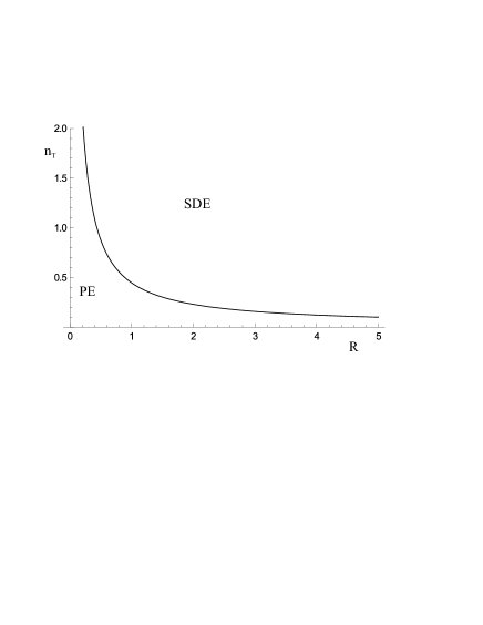
Figure 1: Representation of the asymptotic states determined by reservoir parameters $n_{T}$ and $R$ with respect to their entanglement, for $r=1$ and arbitrary $\phi$. Below the curve, they are entangled, and above, separable. This also determines the asymptotic properties for the entanglement dynamics of any initial state: for points above the curve, every initially entangled state exhibits SDE; for points below the curve, every initial state has some entanglement for large times; and for points exactly in the curve, entanglement can die at finite time or asymptotically.

Since the asymptotic states here obtained are also symmetric, we can apply Eq. (10) to calculate their entanglement of formation. In Fig. 2, we show their values as functions of $R$ for some fixed values of $n_{T}$. For null temperature, when there is no thermal photon, the entanglement is positive for any rate. However, for each positive temperature, there is a maximal rate above which the state is deep separable (as the coupling to the natural reservoir grows, thermal effects are more sensible) corresponding to the regime where the system exhibit SDE.

Figure 2: Entanglement of the asymptotic state as function of the ratio $R=\lambda/\kappa$ between the reservoir’s coupling constants for some values of the number of thermal photons, $n_{T}$, with $r=1$ and arbitrary $\phi$. While the entanglement is always positive for $n_{T}=0$, if $n_{T}>0$ there is always some value of $R$ above which the entanglement is zero.

III.2 Non-asymptotic dynamics

We will discuss here in more detail the system intermediate dynamics. This task is facilitated recognizing, by Eqs. (17), that the dynamics will always describe a straight line in the space of the parameters of the CM ($n_{1},n_{2}$, etc.), for every initial GS, and that the set of separable states is convex for these parameters also. In other words, the trajectories of the CM are given by straight line segments exponentially approaching the asymptotic CM, $V_{\hat{\rho}_{f}}$. From now on we set $\phi=0$, for simplicity in the analysis.

We begin with the situation where the reservoir parameters satisfy Eq. (23) so that the corresponding asymptotic state rests in the border between the separable and entangled sets. If we restrict our attention to initial states with CM, where $n_{1}=n_{2}=n$, $m_{c}$ is real and all other elements are null, Eqs. (17) keep the dynamics inside this same subset. In Fig. 3, we plot a diagram representing the values of $n,m_{c}$ such that the corresponding CM is nonphysical, separable or entangled.

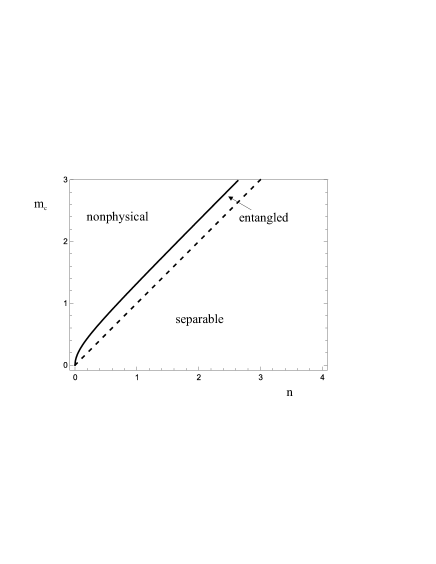
Figure 3: Representation of the CM’s with $n_{1}=n_{2}=n$, $m_{c}\geq 0$ and all other elements equal to zero. The region where these parameters represents physical CM’s is divided by a straight line, above which all states are entangled, while below they are separable. Both regions are convex in the parameters.

The frontier between separable and entangled states is given by the straight line $n=m_{c}$, so the entangled region is convex in these parameters, and by our choice an asymptotic state is defined by the dynamics somewhere in this line. A simple picture of the dynamics can be given for these states, using the fact that the trajectory in the $n\times m_{c}$ space will be a straight line, from the values $(n_{0},m_{c,0})$ of the initial state to the asymptotic values $(n_{f},m_{c,f})$, defined by reservoir parameters $r$ and $R$ [with $n_{T}$ given by Eq. (23)]. If these parameters are such that $\left(n_{0},m_{c,0}\right)$ represents an entangled state, since $\left(n_{f},m_{c,f}\right)$ belongs to the line $n=m_{c}$, the entire trajectory will be on the entangled-state region, by convexity, i.e. entanglement will vanish asymptotically. To illustrate this, we plot in Fig. 4 (dashed line) the evolution of the $S$ function, parametrized by $p(t)=1-\exp{[-2(\kappa+\lambda)t]}$, for an initial state with $n_{0}=1$ and $m_{c,0}=1.0125$ and an asymptotic state with $n_{f}=m_{c,f}=1$. Its value is initially negative, since the initial state is entangled, and remains negative for all times.

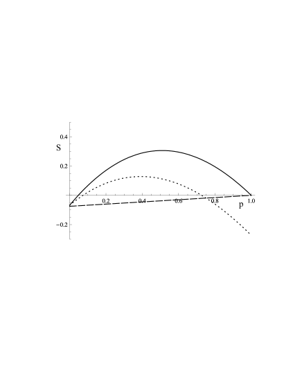
Figure 4: Evolution of the Simon function $S$, parametrized by $p(t)$ for three distinct situations. The continuous line corresponds to an initially entangled state, which enters in the separable region at finite time and converges to an asymptotic state in the frontier. The dotted line is for the same initial state, but the reservoir is such that its corresponding asymptotic state is entangled, with the system losing all its entanglement to recover it later. Finally, the dashed line corresponds to a situation of asymptotic death of entanglement.

For examples of entanglement sudden death, consider the set of states with $n_{1}=n_{2}=n$, $m_{c}=1$ and $m_{1}=m_{2}=m$ a real number. In Fig. 5, we exhibit a diagram analogous to the one in Fig. 3, and we see that the subset of entangled states is not convex anymore. If the asymptotic state also has $m_{c}=1$, the trajectory of the state CM can be described in this diagram and will be again a straight line. Since the entangled region is not convex, we may have initially entangled states that will lose all entanglement at finite time, even if the asymptotic state is in the frontier between the regions.

Figure 5: Representation of the CM’s with $n_{1}=n_{2}=n$, $m_{1}=m_{2}=m\geq 0$, $m_{c}=1$ and all other elements equal to zero. The region where these parameters represents physical CM’s is divided by the dashed curve, above which all states are entangled, while below they are separable. Now the entangled region is not convex in the parameters.

For instance, we can take parameters for the reservoir such that $n_{f}=m_{c,f}=1$ and an initial CM that has elements $n_{0}=1.2$, $m_{0}=0.5$, and $m_{c,0}=1$. In Fig. 4 (continuous line), we plot, as before, the function $S$ of the evolved state. We see that it is initially negative, representing an entangled state, it became positive at finite time, so the state has no entanglement, and it remains strictly positive until it vanishes for $p=1$ (or $t\rightarrow\infty$), because the state converges to a point in the frontier.

If we perturb a little the reservoir parameters so that this asymptotic state becomes entangled, and taking the same initial state, the curve in the figure will be slightly distorted but now will cross the $p$ axis twice, meaning that the state loses all entanglement suddenly but recovers it a later time, remaining entangled for the rest of the dynamics, a possibility mentioned before (see the dotted line of Fig. 4, with the parameters $n_{f}=0.95$ and $m_{c,f}=1$ for the asymptotic state). This is a consequence of the fact that the set of entangled states is not convex on these parameters. Cycles of birth and death are not allowed, since a straight line can cross the convex set of separable states only once.

This feature can be understood, from a more physical point of view, considering the entanglement from the perspective of squeezed EPR-like quadratures. Again, the EPR-like operators with least sum of variances values (i.e., the optimum pair for this state) can be found and read $\hat{X}_{1,r^{\prime}}-\hat{X}_{2,r^{\prime}}$ and $\hat{P}_{1,r^{\prime}}+\hat{P}_{2,^{\prime}}$ with $\hat{X}_{i,r^{\prime}}=r^{\prime}\hat{x}_{i}$, $\hat{P}_{i,r^{\prime}}=\hat{p}_{i}/r^{\prime}$ and $r^{\prime}=\sqrt{(n-m-1/2)/(n+m-1/2)}$. But these are not the quadratures “chosen by” the common reservoir to squeeze (being those with $r^{\prime}=1$, since we had set $\phi=0$). So, on its way to squeezing its favorites, it enlarges the ones from the initial state, such that there is a period of time when no pair of EPR-like quadratures at all are squeezed enough to entangle the modes (see Fig. 6).

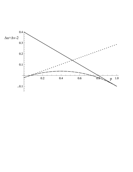
Figure 6: Evolution, parametrized by $p$, for the sum of variances of pairs of EPR quadratures, subtracted by $2$, so that a negative value indicates an entangled state. The continuous, dotted, and dashed curves are, respectively, for the optimum pairs of the final state, the initial state, and the state in each instant of time. We see that the common reservoir enlarges the optimum pair of the initial state to squeeze the pair of the asymptotic state (which is initially large). And there is a period of time where the quadratures with the least sum of variances are not squeezed enough to entangle the states.

It remains then to explore the intermediate dynamics for the situation where the asymptotic state is in the interior of the separables, but this is also easily inferred from the straight line trajectories exhibited by the system: every initial separable state will remain separable for all times, and every initial entangled state will lose its entanglement in finite time.

III.3 Asymmetric engineered reservoir

We have also considered the other extreme case where only one type of atom enters in the cavity, say of type $1$, so that $\kappa_{1}>0$ and $\kappa_{2}=0$ (but again $\lambda_{1}=\lambda_{2}=\lambda$). Here, the second momenta equations of motion read:

$$\dot{n_{1}} = -2(A^{2}\kappa+\lambda)n_{1}+(AB\kappa)m_{c}+$$ (24a)

$$+(AB^{*}\kappa)m_{c}^{*}+2\lambda n_{T},$$

$$\dot{n_{2}} = -2(\lambda-|B|^{2}\kappa)n_{1}-m_{c}(AB\kappa)-$$ (24b)

$$-(AB^{*}\kappa)m_{c}^{*}+2\lambda n_{T}+2\kappa|B|^{2},$$

$$\dot{m_{1}} = -2(A^{2}\kappa+\lambda)m_{1}-(2AB^{*}\kappa)m_{s},$$ (24c)

$$\dot{m_{2}} = -2(\lambda-|B|^{2}\kappa)m_{2}+(2AB^{*}\kappa)m_{s}^{*},$$ (24d)

$$\dot{m_{c}} = -(\kappa+2\lambda)m_{c}-(AB^{*}\kappa)n_{1}+$$ (24e)

$$+(AB^{*}\kappa)n_{2}+AB^{*}\kappa,$$

$$\dot{m_{s}} = -(\kappa+2\lambda)m_{s}+(AB\kappa)m_{1}-(AB^{*}\kappa)m_{2}.$$ (24f)

Despite the asymmetry of the master equation here, the asymptotic states have the same qualitative behavior as in the previous case: for null temperature it will be entangled for any value of $R=\kappa_{1}/\lambda$ but for finite temperature it is separable for high enough $R$. In Fig. 7, we plot the diagram analogous to the one in Fig. 1, determining the dynamical phases for the entanglement dynamics, also separated by a curve with a similar shape.

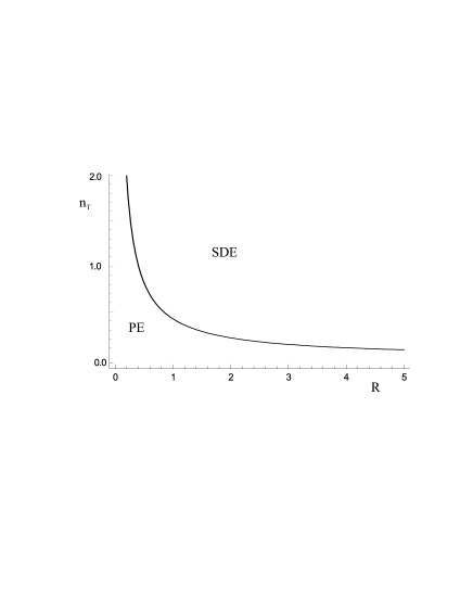
Figure 7: Phase diagram for the asymmetric reservoir, exhibiting the same qualitative behavior as in the symmetric case.

The asymptotic states entanglement, using now the log-negativity for asymmetric GS negcv , are also shown (Fig. 8) for distinct values of $n_{T}$, as function of $R$, and the same interpretation applies here.

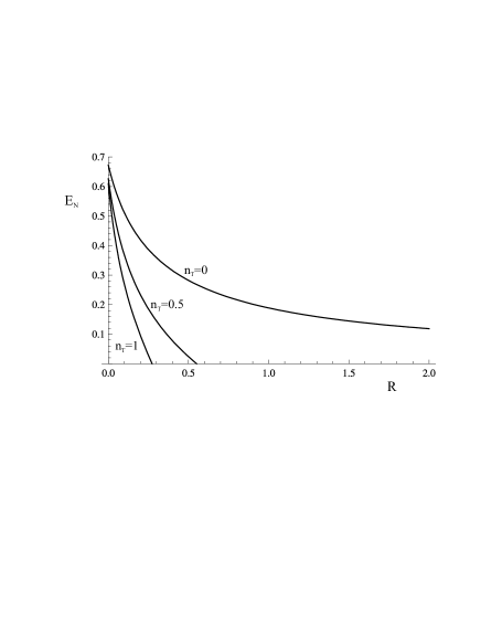
Figure 8: Log-negativity of the asymptotic state for the values $r=1$, and some values of $n_{T}$.

Analogous results are valid also when $\kappa_{2}>0$ but $\kappa_{1}\neq\kappa_{2}$. So, as far as asymptotic issues are concerned, the system presents the same general behavior for both symmetric and asymmetric reservoirs. However, the non-asymptotic analysis made before for the symmetric reservoir becomes much more involved for the asymmetric one, and will be subject of future work.

IV Experimental Proposal

The dynamics studied here is simpler than that in Ref. PR (e.g. being Markovian), yet it is much more controllable and with clear experimental motivation. In this section, we discuss in more detail how to test these predictions in the laboratory.

Considering the state evolution in the laser reference frame, Eqs. (17) will be replaced by

$$\dot{n_{j}} = -2(\kappa+\lambda)n_{j}+2\kappa|B|^{2}+2\lambda n_{T},$$ (25a)

$$\dot{m_{j}} = -2(\kappa+\lambda)m_{j}+(-1)^{j+1}2idm_{j},$$ (25b)

$$\dot{m_{c}} = -2(\kappa+\lambda)m_{c}+2\kappa AB^{*},$$ (25c)

$$\dot{m_{s}} = -2(\kappa+\lambda)m_{s}+2idm_{s},$$ (25d)

where only the equations for $m_{j}$ and $m_{s}$ have changed. If we consider the initial GS where $m_{j}=m_{s}=0$, as well as null amplitudes, the evolution will be the same as that for the interaction picture, i.e., given by Eq.(16), and the coarse graining in time will not affect these states throughout the evolution. For other initial states, the coarse graining will be a source of decoherence, and the state may even lose the Gaussian character along the evolution (like a one-mode coherent state, with non-vanishing amplitude, averaged over its phase).

Our proposal starts then from the preparation of a highly entangled state using the common symmetric reservoir davidov for a total time much shorter than $\lambda^{-1}$, and setting $R\ll 1$ in order to make thermal effects negligible. After the preparation time, the parameter $R$ is set to values of the order $R\gtrapprox 1$, by changing the flux of atoms through the cavity . The system is allowed to evolve until some time $t$ (of the order $\lambda^{-1}$) and the entanglement evolution can be studied, for example, by using the method proposed in Ref. marcelin , to reconstruct the two-mode state. Naturally, one could also try to measure some entanglement witness to simplify the experimental procedure, by using the previous knowledge of the field to reduce the amount of experimental data, but still characterize its entanglement.

For this setting, i.e., assuming an initial two-mode squeezed state, the times where entanglement sudden death (ESD) takes place can be obtained explicitly and reads:

$$\lambda t_{ESD}=\frac{R}{2(1+R)}\ln{(1-p_{ESD})^{-1}},$$ (26)

where

$$p_{ESD}=\frac{(1+R)(B^{2}-AB)}{(1+R)(B^{2}-AB)-B^{2}-n_{T}R+AB},$$ (27)

and the parameter $R$ refers to the one in the second stage of the procedure, after the initial state preparation. These times, in units of $\lambda^{-1}$, are exhibited as function of $R$ in Fig. 9, for some values of temperature. Naturally, they are infinite for small $R$, in the region where persistent entanglement takes place. After the threshold, it falls abruptly and stabilizes in values close to unity, so the entanglement will typically survive long enough for its (not so sudden) death to be observed. It may also be interesting to study thermal effects like the behavior of $\frac{dE_{F}}{dt}$ before the sudden death, which is an indicator of the incidence of the dynamical trajectory of $\hat{\rho}$ at the set of separable states, by controlling the temperature.

Figure 9: Sudden death time as function of $R$, for some values of $n_{T}$. It is infinite for small $R$, corresponding to the persistent entanglement region, but after the threshold, it rapidly falls to a value near to unity.

V Robustness of the Scheme for Generating Entangled GS in a Cavity

Since entanglement in GS is related to squeezing in the proper EPR quadratures, while the natural thermal effect is to spread Wigner functions, it is in order to ask about the sensibility of the preparation scheme with natural dissipation, considering the regime $R\ll 1$ and $n_{T}\ll 1$. Actually we have analyzed a slightly different procedure than the original one by Pielawa et al. davidov . There they propose to empty the modes $\hat{b}_{j}$ at turns, passing a stream of atoms of type $1$, say, until mode $\hat{b}_{1}$ is sufficiently “washed”, then repeating the procedure with type $2$ atoms. Here we consider that both types of atoms can pass through the cavity, not at the same time, but with equal probability, so that we can apply the equations for the symmetric reservoir to compute the system evolution.

Supposing that the two original modes, $\hat{a}_{i}$, are initially empty (and remembering that the number of photons can be lower than the number of thermal photons if one passes a suitable stream of atoms to “steal” photons from the mode), the evolution of the covariance matrix of the system will be then given with the following non-zero entries: $n_{1}=n_{2}=\frac{|B|^{2}+n_{T}R}{1+R}p(t)$ and $m_{c}=\frac{AB}{1+R}p(t)$, where again $p(t)=(1-\exp{[-2(\kappa+\lambda)t]})$. Assuming also that the duration of experiment $t$ is large enough so that $p\approx 1$ (which can be achieved with $t\gg\kappa^{-1}$ but still $t\ll\lambda^{-1}$) or, in other words, that the system is essentially in the asymptotic state of the procedure, we plot in Fig. 10 the entanglement of formation as a function of $R$, for $n_{T}=0.05$ (value attained in the recent experiment reported in Ref. expharoche ) for distinct values of $r$.

Figure 10: Entanglement of the asymptotic states as function of the ratio $R=\lambda/\kappa$ between the reservoir decay rates, for some values of squeezing parameter $r$, with $n_{T}=0.05$, normalized by its value at $R=0$. The continuous line is for $r=1$, dotted for $r=1.5$, dashed for $r=2$ and dotted-dashed for $r=2.5$. The entanglement is somewhat sensitive to dissipation, and is more sensitive the greater the squeezing parameter.

The graphs are normalized by the value of the entanglement of formation with $R=0$, which would be obtained if there were no dissipation. We see that the entanglement is somewhat sensitive to the dissipation, even at such a low temperature, and can be lowered by half, for $R=0.1$, i.e. , when the engineered reservoir rate is ten times greater then the dissipation rate. Also, the greater the squeezing parameter, the sensitive entanglement becomes to dissipation, as expected. Though, if $\kappa$ is above two orders of magnitude greater than $\lambda$, the entanglement does not appear to be significantly changed. For a squeezing parameter of $r=1$, a value of $R\approx 10^{-2}$ and a waiting time of about $3\kappa^{-1}$ would suffice to obtain an amount of entanglement greater than $90\%$ of the pure ideal state (with $R=0$ and infinite waiting time).

VI Conclusion

An engineered reservoir can be used to create entangled states of two field modes in a cavity davidov . We here show that it can also be used, together with the natural thermal reservoir, to depict asymptotic entanglement phase diagrams PR . Taking advantage of the fact that the specific reservoirs used preserve Gaussianity, we could make all the discussion of entanglement in terms of covariance matrices. We showed that only two behaviors are allowed: asymptotic entanglement or entanglement “sudden death”. The line between both phases allows the coexistence of both behaviors.

Besides asymptotic studies, the symmetric engineered reservoir was also studied in detail, with examples of all possible entanglement fates exhibited.

This study can be viewed as an experimental proposal for drawing entanglement phase diagrams and for monitoring the “transition”. Another byproduct is the study of the robustness of the proposal for entanglement generation with respect to the natural thermal environment. An interesting question raised is what would be the best setup for such experimental drawing of asymptotic entanglement phase diagrams.

The authors thank S. Pielawa, M. F. Santos and J. P. Paz for helpful comments and suggestions. We are grateful for the support of Brazilian agencies CNPq and Fapemig. This work is part of Brazilian National Institute for Science and Technology on Quantum Information. R.C.D. was supported also by CAPES, Proc.: BEX 0124/10-9.

References

- (1) K. Życzkowski, P. Horodecki, M. Horodecki, and R. Horodecki, Phys. Rev. A65, 012101 (2001); T. Yu and J. H. Eberly, Phys. Rev. B66, 193306 (2002); L. Diósi, Lect. Notes Phys. 622, 157 (2003); P. J. Dodd and J. J. Halliwell, Phys. Rev. A69, 052105 (2004); T. Yu and J. H. Eberly, Opt. Commun. 264, 393 (2006).
- (2) D. Gross, S. T. Flammia, and J. Eisert, Phys. Rev. Lett. 102, 190501 (2009); M. J. Bremner, C. Mora, and A. Winter, Phys. Rev. Lett. 102, 190502 (2009); D. Bacon, Physics 2, 38 (2009).
- (3) A. Serafini, F. Illuminati, M. G. A. Paris and S. De Siena, Phys. Rev. A69, 022318 (2004); S. Maniscalco, S. Olivares, and M. G. A. Paris, Phys Rev. A 75, 062119 (2007); C.-H. Chou, T. Yu, B. L. Hu, Phys. Rev. E 77, 011112 (2008); F. Benatti and R. Floreanini, J. Phys. A: Math. Theor. 39, 2689 (2006).
- (4) M. O. Terra Cunha, New J. Phys. 9, 237 (2007); R. C. Drumond and M. O. Terra Cunha, Foundations of Probability and Physics-5, American Institute of Physics Conference Proceedings, 1101, 386 New York (2009); R. C. Drumond and M. O. Terra Cunha, J. Phys. A: Math. Theor. 42, 285308 (2009).
- (5) J. P. Paz and A. J. Roncaglia, Phys. Rev. Lett. 100, 220401 (2008); Phys. Rev. A79, 032102 (2009).
- (6) S. Pielawa, G. Morigi, D. Vitali and L. Davidovich, Phys. Rev. Lett. 98, 240401 (2007).
- (7) C. H. Bennett, G. Brassard, C. Crépeau, R. Jozsa, A. Peres, W. K. Wootters, Phys. Rev. Lett. 70, 1895 (1993).
- (8) S.L. Braunstein and H.J. Kimble, Phys. Rev. Lett. 80, 869 (1998).
- (9) A. K. Ekert, Phys. Rev. Lett. 67, 661 (1991).
- (10) M.D. Reid, Phys. Rev. A62, 062308 (2000); M. Hillery, Phys. Rev. A61, 022309 (2000); T. C. Ralph, Phys. Rev. A61, 010303(R) (1999).
- (11) Ch. Silberhorn, T. C. Ralph, N. Lutkenhaus, and G. Leuchs, Phys. Rev. Lett. 89, 167901 (2002).
- (12) A. Peres, Phys. Rev. Lett. 77, 1413 (1996).
- (13) M. Horodecki, P. Horodecki, R. Horodecki, Physics Letters A 223, 1 (1996).
- (14) R. Simon, Phys. Rev. Lett. 84, 2726 (2000).
- (15) A. Einstein, B. Podolsky, and N. Rosen, Physical Review 47, 777 (1935).
- (16) G. Vidal and R. F. Werner,Phys. Rev. A65, 032314 (2002).
- (17) M. B. Plenio, Phys. Rev. Lett. 95, 090503 (2005).
- (18) C.H. Bennett, D. P. DiVincenzo, J. A. Smolin, and W.K. Wootters, Phys. Rev. A54, 3824 (1996).
- (19) G. Adesso, A. Serafini and F. Illuminati, Phys. Rev. A70 022318 (2004); Phys. Rev. Lett. 93 220504 (2004).
- (20) G. Giedke, M. M. Wolf, O. Krüger, R. F. Werner, and J. I. Cirac, Phys. Rev. Lett. 91, 107901 (2003).
- (21) G. Adesso, PhD. Thesis, Universitá di Salerno (2006), arXiv:quant-ph/0702069.
- (22) L. M. Duan, G. Giedke, J. I. Cirac, and P. Zoller, Phys. Rev. Lett. 84, 2722 (2000).
- (23) G. Rigolin and C. O. Escobar, Phys. Rev. A69, 012307 (2004).
- (24) G. Lindblad, Commun. Math. Phys. 48, 119 (1976).
- (25) B.-G. Englert and G. Morigi, in Coherent Evolution in Noisy Environments, edited by A. Buchleitner and K. Hornberger (Springer, Berlin, 2002), p. 55.
- (26) M. França Santos, L. G. Lutterbach, and L. Davidovich, J. Opt. B: Quantum Semiclass. Opt. 3, S55 (2001).
- (27) M. Brune, J. Bernu, C. Guerlin, S. Deleglise, C. Sayrin, S. Gleyzes, S. Kuhr, I. Dotsenko, J. M. Raimond, and S. Haroche Phys. Rev. Lett. 101, 240402 (2008).