The Phase Behaviors of A Polymer Solution Confined between Two Concentric Cylinders

Abstract

A theoretical study on the phase behaviors of a polymer solution confined between two coaxial cylindrical walls is presented. For the case of a neutral inner cylinder, the spinodal point derived through the Gaussian fluctuation theory is confinement-independent because of the existence of a free dimension in the system. The kinetic analysis indicates that the fluctuation modes always have a component of a plane wave along the axial direction, which can lead to the formation of a periodic-like concentration pattern. On the other hand, the equilibrium structure of the system is obtained by using the self-consistent mean-field theory (SCMFT) and the interplay between the “wetting” phenomenon and the phase separation is observed by modifying the property of the inner cylinderical wall.

I introduction

Rigorously speaking, the classical thermodynamics should be always used to deal with the systems of infinite particles in an inifinite space. For a real finite system with a large amount of particles, the classical thermodynamic treatment is valid when the dimension of the confinement is much larger than the characteristic length of the system. Otherwise, the boundary of the system will cause obvious effects on the interior behaviors.

For a binary fluid mixture, an important characteristic length scale is the correlation length, which will become infinite when the system approaches the critical state. Hence, the phase behavior of a confined binary fluid mixture can be affected much by the boundary of the system. Two common kinds of confinement are film and porous media, which correspond to the flat boundary case and the curved boundary case, respectively. The former is always modeled as a system confined between two slabs. For this case, when the system is quenched into the unstable region, the composition fluctuations with characteristic wave vectors parallel to the slabs can grow unrestrictedly while the ones with perpendicular wave vectors will be modulated by the confinement. As a result, the microphase structure in the system must coarsen laterally after the intermediate stage of the phase separation and the power law of the domain growth is different from the bulk case Binder (1998); Wang and Composto (2000); Tanaka and Araki (2000); Wanga and Mashita (2004); Rysz (2005); Yao et al. (2005). In addition, each slab can be neutral or preferential to a certain component of the mixture so that the phase behavior can be coupled with the wetting phenomenon Tanaka (1993a); Wendlandt et al. (2000); Das et al. (2006a, b); Binder et al. (2008). Compare to the flat boundary case, the porous media is much more complicated. The simplest model for this case is a binary system confined inside a cylindrical pore. Because there is only one free dimension for the cylindrical pore, the time required by the system to reach equilibrium is always so long that some metastable states are long-lived. The wetting behavior also has great importance to the phase behavior for this case Liu et al. (1990); Liu and Grest (1991); Monette et al. (1992); Tanaka (1993b); Zhang and Chakrabarti (1994, 1995); Woywod et al. (2005).

Another interesting case is considered in this work. That is a polymer solution confined between two concentric cylindrical walls. This kind of confinement can be regarded as a combination of the two that mentioned in the last paragraph and hence is more general. When the radius of the inner cylinder converges to zero, the system will reduce to the one in a cylindric pore. On the other hand, if the radii of the two cylinders converge to infinite with a constant width between the two walls, the system will reduce to the one confined between two slabs. Thus, many results of this work can be easily generalized to the two limiting cases. In addition, a polymeric system is always a good object for studying phase behaviors theoretically because the polymer chain length is a natural long enough length scale which makes the coarse-grained treatment and mean-field theory strictly valid.

In the present work, we give a theoretical study on the phase behaviors of a polymer solution confined between two coaxial cylindrical walls. The self-consistent mean-field theory (SCMFT) is used to investigate the equilibrium structure of the system. The spinodal point of the system is determined by using the Gaussian fluctuation theory. The kinetics of the system are also studied by combining SCMFT with the Cahn-Hilliard theory.

II theoretical framework

Consider a polymer solution confined between two infinit long coaxial cylindrical walls, as illustrated in Fig. 1. The inner cylinder has the radius $r$ and the outer one has radius $R$. The average volume fraction of the polymer is $\overline{\phi}_{\rm P}$, and that of the solvent is $\overline{\phi}_{\rm S}=1-\overline{\phi}_{\rm P}$. The canonical ensemble is used here, and the free energy of the system can be derived by the self-consistent mean-field theory Yang et al. (2006a); Man et al. (2008),

$$\frac{F}{\rho_{{}_{\scriptstyle 0}}} = \chi\int{\rm d}\mathbf{r}\phi_{\rm P}(\mathbf{r})\phi_{\rm S}(\mathbf{r})+\int{\rm d}\mathbf{r}U(\mathbf{r})\phi_{\rm P}(\mathbf{r})-\sum_{\alpha}\int{\rm d}\mathbf{r}\omega_{\alpha}(\mathbf{r})\phi_{\alpha}(\mathbf{r})$$ (1)

$$-\frac{V\overline{\phi}_{\rm P}}{N}\ln\frac{z_{0\rm P}NeQ_{\rm P}}{\rho_{{}_{\scriptstyle 0}}\overline{\phi}_{\rm P}}-V\overline{\phi}_{\rm S}\ln\frac{z_{0\rm S}eQ_{\rm S}}{\rho_{{}_{\scriptstyle 0}}\overline{\phi}_{\rm S}}$$

In Eq. (1), $\rho_{{}_{\scriptstyle 0}}$ is the monomer density, which is defined as monomers per unit volume; $\alpha=\mbox{P,\,S}$; $\chi$ is the Flory-Huggins parameter, which quantifies the local interaction between each pair of polymer segments and solvent molecules; $\phi_{\alpha}(\mathbf{r})$ is the volume fraction of species $\alpha$ at point $\mathbf{r}$ ; $\omega_{\alpha}(\mathbf{r})$ is the auxiliary field conjuncted to $\phi_{\alpha}(\mathbf{r})$; $N$ is the degree of polymerization; $z_{0\alpha}$ is the partition function of component $\alpha$ due to the kinetic energy, which can be regarded as a constant; $Q_{\alpha}$ is the partition function of a single molecule of component $\alpha$. $U(\mathbf{r})$ is the effective adsorbing potential to the polymers, which is assumed to be a rectangular-form potential for simplicity and is just put on the inner cylindrical wall in the present calculations. It is convenient to use cylindrical coordinates here and after. Then, $U(\mathbf{r})$ has the form

$$U(\rho,\,z)=\left\{\begin{array}[]{c@{\quad}l}-U_{0}&r<\rho\leq r+d\\ 0&r+d<\rho<R\end{array}\right.$$ (2)

where $U_{0}$ is a constant which quantifies the strength of the potential; $d$ is the force range of the potential. To obtain the free energy, we need to solve a set of SCMFT equations,

$$\phi_{\rm P}(\rho,\,z)=\frac{\overline{\phi}_{\rm P}}{NQ_{\rm P}}\int_{0}^{N}{\rm d}tq(\rho,\,z,t)q(\rho,\,z,N-t)$$ (3)

$$\phi_{\rm S}(\rho,\,z)=\frac{\overline{\phi}_{\rm S}}{Q_{\rm S}}e^{-\omega_{{}_{\rm S}}(\rho,\,z)}$$ (4)

$$\omega_{{}_{\scriptstyle\rm P}}(\rho,\,z)=\chi\phi_{\rm S}(\rho,\,z,t)+U(\rho,\,z)+\eta(\rho,\,z)$$ (5)

$$\omega_{{}_{\scriptstyle\rm S}}(\rho,\,z)=\chi\phi_{\rm P}(\rho,\,z,t)+\eta(\rho,\,z)$$ (6)

$$\phi_{\rm P}(\rho,\,z,t)+\phi_{\rm S}(\rho,\,z,t)=1$$ (7)

Because the system has a rotational symmetry about the $z$-axis, the position-dependent functions in the SCMFT equations are independent on the polar angle. In Eq. (3), $t$ is the coordinate along a polymer chain; the end-integrated propagators, $q(\rho,\,z,t)$, satisfies the modified diffusion equation

$$\frac{\partial q(\rho,\,z,t)}{\partial t}=\frac{b^{2}}{6}\left[\frac{1}{\rho}\frac{\partial}{\partial\rho}\left(\rho\frac{\partial}{\partial\rho}\right)+\frac{\partial^{2}}{\partial z^{2}}\right]q(\rho,\,z,t)-\omega_{{}_{\scriptstyle\rm P}}(\rho,\,z)q(\rho,\,z,t)$$ (8)

with the initial condition, $q(\rho,\,z,0)=1$. All lengths in the present calculations are scaled by the Kuhn length $b$ of the polymer, and thus $b=1$ in Eq. (8). It should be pointed out that, to derive the above equations, the well-known Wiener measure is used to depict the conformation of each polymer chain. Hence our calculation should be restricted in the weak confinement case, i.e. $R-r>R_{g}$ where $R_{g}=(\frac{1}{6}N)^{1/2}b$.

According to the Gaussian fluctuation theory Shi (2004), when there exists some fluctuations around the mean-field state, i.e. $\phi_{\alpha}(\mathbf{r})=\phi_{\alpha}^{(0)}(\mathbf{r})+\delta\phi_{\alpha}(\mathbf{r})$ , the free energy of the system can be written as an expansion

$$F=F^{(0)}+F^{(1)}+F^{(2)}+\cdots$$ (9)

where $F^{(0)}$ is the mean-field free energy illustrated by Eq. (1); $F^{(1)}=0$ since the mean-field solution satisfies the SCMFT equations; $F^{(2)}$ has the form as

$$F^{(2)}=\frac{1}{2}\ln\left\{\det\left[\left(\frac{\rho_{{}_{\scriptstyle 0}}}{\pi}\right)^{2}C\cdot\tilde{C}\right]\right\}-\ln\int\mathcal{D}\{\delta\phi\}e^{-\mathcal{F}^{(2)}[\{\delta\phi\}]}$$ (10)

In Eq. (10), the first term has no direct relations with current discussions; the functional $\mathcal{F}^{(2)}[\{\delta\phi\}]$ in the second term is given by

$$\mathcal{F}^{(2)}[\{\delta\phi\}]=\frac{\rho_{{}_{\scriptstyle 0}}}{4}\int{\rm d}\mathbf{r}{\rm d}\mathbf{r}^{\prime}(C^{\rm RPA})^{-1}(\mathbf{r},\mathbf{r}^{\prime})\delta\phi(\mathbf{r})\delta\phi(\mathbf{r}^{\prime})$$ (11)

where $\delta\phi(\mathbf{r})=\delta\phi_{\rm P}(\mathbf{r})-\delta\phi_{\rm S}(\mathbf{r})$. The inverse of the RPA two-point correlation function in Eq. (11), $(C^{\rm RPA})^{-1}(\mathbf{r},\mathbf{r}^{\prime})$, is defined as

$$(C^{\rm RPA})^{-1}(\mathbf{r},\mathbf{r}^{\prime})=\widetilde{C}^{-1}(\mathbf{r},\mathbf{r}^{\prime})-\chi\delta(\mathbf{r}-\mathbf{r}^{\prime})$$ (12)

where

$$\widetilde{C}(\mathbf{r},\mathbf{r}^{\prime})=C(\mathbf{r},\mathbf{r}^{\prime})-\int{\rm d}\mathbf{r}_{1}{\rm d}\mathbf{r}_{2}\Delta(\mathbf{r},\mathbf{r}_{1})C^{-1}(\mathbf{r}_{1},\mathbf{r}_{2})\Delta(\mathbf{r}_{2},\mathbf{r}^{\prime})$$ (13)

In these expressions, the inverse operaters are defined through the relation $\int{\rm d}\mathbf{r}_{1}O^{-1}(\mathbf{r},\mathbf{r}_{1})O(\mathbf{r}_{1},\mathbf{r}^{\prime})=\delta(\mathbf{r}-\mathbf{r}^{\prime})$; the formulas of $C(\mathbf{r},\mathbf{r}^{\prime})$ and $\Delta(\mathbf{r},\mathbf{r}^{\prime})$ can be found in ref. Shi (2004).

Many thermodynamic information of the system can be obtained from $(C^{\rm RPA})^{-1}(\mathbf{r},\mathbf{r}^{\prime})$. Particularly, the condition that the smallest eigenvalue of $(C^{\rm RPA})^{-1}(\mathbf{r},\mathbf{r}^{\prime})$ determines the spinodal point. In principle, the eigenvalues of $(C^{\rm RPA})^{-1}(\mathbf{r},\mathbf{r}^{\prime})$ can be derived by solving the eigenvalue problem

$$\int{\rm d}\mathbf{r}^{\prime}(C^{\rm RPA})^{-1}(\mathbf{r},\mathbf{r}^{\prime})\Psi_{n}(\mathbf{r}^{\prime})=\lambda_{n}\Psi_{n}(\mathbf{r})$$ (14)

where $n$ denotes a complete set of quantum numbers.

III results and discussions

III.1 The case of neutral cylinderic walls

In this section, we mainly focus on the case of neutral cylindrical walls, i.e. $U_{0}=0$. Because we always have $R-r\gg b$ in this work, the boundary layers between the bulk of the polymer solution and the two cylindrical walls are less important. Thus it is reasonable to omit the boundary layers by letting $q(\rho,\,z,t)$ satisfy the free boundary condition, i.e. $\left.\frac{\partial q_{{}_{\rm P}}}{\partial\rho}\right|_{\rm boundry}=0$. After these treatments, it can be seen that the SCMFT equation set has a solution for a homogeneous phase, in which $\phi_{\rm P}(\rho,\,z)=\overline{\phi}_{\rm P}$ and $\phi_{\rm S}(\rho,\,z)=\overline{\phi}_{\rm S}$. This trivial solution represents the equilibrium structure of the system when $\chi$ is small. However, fluctuations will ultimately destroy the homogeneity of the system with the increasing of $\chi$. As mentioned above, the critical point at which the system becomes unstable (i.e. the spinodal point) can be derived from $(C^{\rm RPA})^{-1}(\mathbf{r},\mathbf{r}^{\prime})$. Rather than solve the eigenvalue problem in Eq. (14) directly, it is more convenient to expand $(C^{\rm RPA})^{-1}(\mathbf{r},\mathbf{r}^{\prime})$ with the eigenfunctions of the Laplacian operator, $\nabla^{2}$. For the geometry of the system considered here, the eigenfunctions of $\nabla^{2}$ are given by

$$\psi_{nmk}(\rho,\theta,z)=A_{nmk}R_{nm}(\rho)e^{im\theta}e^{ikz}$$ (15)

with the eigenvalues

$$\lambda_{nmk}=(\epsilon_{n}^{|m|})^{2}+k^{2}$$ (16)

where $A_{nmk}$ is the normalization factor; $|m|=0,1,2,\ldots$; $n=1,2,\ldots$; $k$ is the one-dimensional continuous wave vector along $z$-direction. In Eq. (16), $\epsilon_{n}^{|m|}$ can be zero or non-zero; when it is non-zero, according to the boundary condition, it is the $n$-th root of the following equation

$$\left|\begin{array}[]{c@{\quad}c}J_{|m|}^{\prime}(\epsilon_{n}^{|m|}r)&N_{|m|}^{\prime}(\epsilon_{n}^{|m|}r)\\ J_{|m|}^{\prime}(\epsilon_{n}^{|m|}R)&N_{|m|}^{\prime}(\epsilon_{n}^{|m|}R)\end{array}\right|=0$$ (17)

where $J_{|m|}(x)$ and $N_{|m|}(x)$ are the $|m|$-th order Bessel function and the $|m|$-th order Neumann function, respectively. The radial part of the eigenfunction in Eq. (15), $R_{nm}(\rho)$, is

$$R_{nm}(\rho)=\left\{\begin{array}[]{l@{,\quad}l}\delta_{m,0}&\epsilon_{n}^{|m|}=0\\ J_{|m|}(\epsilon_{n}^{|m|}\rho)-\frac{J_{|m|}^{\prime}(\epsilon_{n}^{|m|}r)}{N_{|m|}^{\prime}(\epsilon_{n}^{|m|}r)}N_{|m|}(\epsilon_{n}^{|m|}\rho)&\epsilon_{n}^{|m|}\neq 0\end{array}\right.$$ (18)

Expanding $(C^{\rm RPA})^{-1}(\mathbf{r},\mathbf{r}^{\prime})$ by $\{\psi_{nmk}\}$ leads to

$$(C^{\rm RPA})^{-1}(\mathbf{r},\mathbf{r}^{\prime})=\sum_{nmk}a_{nmk}\psi_{nmk}^{*}(\mathbf{r}^{\prime})\psi_{nmk}(\mathbf{r})$$ (19)

The expansion coefficient is given by

$$a_{nmk}=\frac{1}{2\overline{\phi}_{\rm S}}+\frac{\lambda_{nmk}}{4\overline{\phi}_{\rm P}[1-g(\lambda_{nmk}N)]}-\chi$$ (20)

where $g(x)=\frac{1-e^{-x}}{x}$. As can be seen obviously from Eq. (19), the eigenfunctions of $(C^{\rm RPA})^{-1}(\mathbf{r},\mathbf{r}^{\prime})$ are also $\{\psi_{nmk}\}$ with the eigenvalues ${a_{nmk}}$. Hence, the spinodal point can be derived from Eq. (20) that

$$\chi_{{}_{\rm SP}} = \min\left\{\frac{1}{2\overline{\phi}_{\rm S}}+\frac{\lambda_{nmk}}{4\overline{\phi}_{\rm P}[1-g(\lambda_{nmk}N)]}\right\}$$ (21)

$$= \frac{1}{2}\left(\frac{1}{\overline{\phi}_{\rm S}}+\frac{1}{N\overline{\phi}_{\rm P}}\right)$$

Obviously, this result is the same as the non-confined case and is consistent with other related works Miao et al. (2006). Physically speaking, the $z$-direction is a free dimension, thus the system can undergo phase separations along this direction with no confinement, which is refflected by the confinement-independent spinodal point.

It is worth noting that the mode corresponding to the minimum eigenvalue of $(C^{\rm RPA})^{-1}(\mathbf{r},\mathbf{r}^{\prime})$ is a constant, which corresponds a global translation of the system. This means that if $\chi$ just equals $\chi_{{}_{\rm SP}}$, the system is in a critical state but with no phase separation. However, once $\chi$ exceeds $\chi_{{}_{\rm SP}}$, many fluctuation modes will be excited to induce the spinodal decomposition in the system. To study these modes in the early-stage of the phase separation, we firstly rewrite the free energy in Eq. (1) to a functional of $\phi_{\rm P}(\mathbf{r})$ by using the slow gradient expansion Fredrickson (2006),

$$F = \int{\rm d}\mathbf{r}\left[\chi\phi_{\rm P}(1-\phi_{\rm P})+\frac{\phi_{\rm P}}{N}\ln\phi_{\rm P}+(1-\phi_{\rm P})\ln(1-\phi_{\rm P})+\frac{1}{36\phi_{\rm P}}(\nabla\phi_{\rm P})^{2}+\cdots\right]+{\rm const}$$ (22)

$$\approx F_{0}+\int{\rm d}\mathbf{r}\left[(\chi_{{}_{\rm SP}}-\chi)(\phi_{\rm P}-\overline{\phi}_{\rm P})^{2}+\frac{1}{36\overline{\phi}_{\rm P}}(\nabla\phi_{\rm P})^{2}\right]$$

where $F_{0}$ is the free energy of the homogeneous state; the constant $\rho_{{}_{\scriptstyle 0}}$ is omitted for simplicity, and the high-order terms are also omitted in the last step. On the other hand, the time evolution of $\phi_{\rm P}(\mathbf{r})$ can be depicted by the Cahn-Hilliard theory Cahn and Hilliard (1958); Cahn (1959); Cahn and Hilliard (1959); Cahn (1965)

$$\frac{\partial\phi_{\rm P}(\mathbf{r},\tau)}{\partial\tau}=\nabla^{2}\left(\frac{\delta F}{\delta\phi_{\rm P}}\right)$$ (23)

where $\tau$ is a scaled time variable. By inserting Eq. (22) into Eq. (23), it can be derived that

$$\frac{\partial\delta\phi_{\rm P}}{\partial\tau}=\nabla^{2}\left[2(\chi_{{}_{\rm SP}}-\chi)\delta\phi_{\rm P}-\frac{1}{18\overline{\phi}_{\rm P}}\nabla^{2}\delta\phi_{\rm P}\right]$$ (24)

where the fluctuation $\delta\phi_{\rm P}=\phi_{\rm P}-\overline{\phi}_{\rm P}$ is used instead of $\phi_{\rm P}$.

Then we expand $\delta\phi_{\rm P}$ by $\{\psi_{nmk}\}$. Because of the axial symmetry of the system, it is only necessary to consider the fluctuation modes which are independent on the polar angle $\theta$. Hence,

$$\delta\phi_{\rm P}=\sum_{nk}c_{nk}(\tau)A_{n0k}R_{n0}(\rho)e^{ikz}$$ (25)

By inserting Eq. (25) into Eq. (24), the evolving equation of the expansion coefficient, $c_{nk}(\tau)$, is derived

$$\frac{\partial c_{nk}}{\partial\tau}=-2(\chi_{{}_{\rm SP}}-\chi)\lambda_{n0k}c_{nk}-\frac{1}{18\overline{\phi}_{\rm P}}\lambda_{n0k}^{2}c_{nk}$$ (26)

The solution of Eq. (26) is

$$c_{nk}(\tau)=c_{nk}(0)e^{\omega_{nk}\tau}$$ (27)

where

$$\omega_{nk} = 2(\chi-\chi_{{}_{\rm SP}})\lambda_{n0k}-\frac{1}{18\overline{\phi}_{\rm P}}\lambda_{n0k}^{2}$$ (28)

$$= 2(\chi-\chi_{{}_{\rm SP}})\left[(\epsilon_{n}^{0})^{2}+k^{2}\right]-\frac{1}{18\overline{\phi}_{\rm P}}\left[(\epsilon_{n}^{0})^{2}+k^{2}\right]^{2}$$

When the system is thermodynamically unstable, $\chi>\chi_{{}_{SP}}$. Then as can be seen from Eq. (28), for $(\epsilon_{n}^{0})^{2}+k^{2}<36\overline{\phi}_{\rm P}(\chi-\chi_{{}_{\rm SP}})$, $\omega_{nk}>0$, and the corresponding fluctuations increase with time. In particular, if

$$(\epsilon_{n}^{0})^{2}+k^{2}=18\overline{\phi}_{\rm P}(\chi-\chi_{{}_{\rm SP}})$$ (29)

$\omega_{nk}$ is maximized, and

$$(\omega_{nk})_{\max}=18\overline{\phi}_{\rm P}(\chi-\chi_{{}_{\rm SP}})^{2}$$ (30)

This value corresponds to a maximum in the rate of increase of concentration fluctuations in the system.

From the discussion above, it can be seen that the possible fluctuation patterns in the unstable system are dependent on $\overline{\phi}_{\rm P}$, $r$, $R$ and $N$. Generally speaking, these patterns have two parts, i.e. a radial part and a part along the $z$-direction, as illustrated by Eq. (25). However, it is interesting that $(\epsilon_{1}^{0})^{2}$ can be larger than $36\overline{\phi}_{\rm P}(\chi-\chi_{{}_{\rm SP}})$ for many combinations of these parameters. For example, when $\overline{\phi}_{\rm P}=0.01$, $r=3$, $R=50$ and $N=600$, $(\epsilon_{1}^{0})^{2}$ is not smaller than $36\overline{\phi}_{\rm P}(\chi-\chi_{{}_{\rm SP}})$ until $\chi$ exceeds 0.8. Note that $R_{0}^{0}(\rho)=1$, then in the above cases, the fluctuation modes that can increase with time must be plane waves along the $z$-direction. This will lead to a periodic-like concentration profile along the $z$-direction in the early stage of the phase separation.

Although the analysis above is in principle just applicable to the early stage of the phase separation in the system, it can indeed be concluded that the phase separation must be along the $z$-direction even in the late stage. This is because the system needs to put the interface vertical to $z$-direction in order to minimize the interface area. As a result, even though the fluctuation mode may have a radial part in the early stage, only the $z$-direction plane wave part can be maintained as time goes by.

III.2 The confined polymer solution with the presence of an adsorbing potential

In this section, $U_{0}$ in Eq. (2) is set to be positive. Hence, there is an adsorbing potential to the polymers at the inner cylindric wall. With the presence of this adsorbing potential, the boundary layer at the inner cylindric wall cannot be omitted and it needs to use the first kind boundary condition for $q(\rho,\,z,t)$, i.e. $q(\rho,\,z,t)|_{\rho=r}=0$, because of the impenetrability of the inner wall. By contrast, the free boundary condition can still be used at the outer wall, i.e. $\left.\frac{\partial q_{{}_{\rm P}}}{\partial\rho}\right|_{\rho=R}=0$. Then the equilibrium structure of the system can be obtained by solving the SCMFT equations numerically. Especially, Eq. (8) is solved by using the alternating direction implicit (ADI) method Roan and Kawakatsu (2002); Yang et al. (2006b).

In the present calculations, $\chi$ is always set to be larger than $\chi_{{}_{\rm SP}}$. As such, one can expect some interplays between the adsorption of the polymer by the inner cylindric wall and the phase separation in the system. The main results are illustrated in Fig. 2. Note that the periodic boundary condition is used along the $z$-direction for convenience in the calculations, but the period along the $z$-direction in Fig. 2 is of no physical meanings. The strength of the adsorbing potential increases gradually from Fig. 2(a) to Fig. 2(c). As can be seen from the figure, when the adsorbing potential is weak, it has few effects on the phase behaviors of the confined solution, and the system separates into a polymer rich phase and a solvent rich phase with the interface being vertical to the $z$-direction. However, accompanying with the increase of the adsorbing strength, a “wetting” layer can be formed by the polymer at the inner cylindric wall, as illustrated in Fig. 2(b). Furthermore, after the strength of the adsorbing potential exceeds a certain threshold, the interface between the polymer rich phase and the solvent rich phase becomes along the $z$-direction and then the concentration profile of the system is independent on $z$ (Fig. 2(c)).

As been discussed in Sec. IIIA, the interface between the polymer rich phase and the solvent rich phase prefers to be vertical to $z$-direction in order to minimize the interface area. However, the $z$-independent adsorbing potential, $U$, dislikes the inhomogeneity along the $z$-direction. The competition between these two factors results in the variations in the concentration profiles, which are illustrated in Fig. 2. This phenomenon is similar to the “plug-tube” transition of a binary liquid mixture in a cylindrical pore. It is worth pointing out that the threshold of $U_{0}$, above which the transition happens, is always not very large, although it is dependent on the parameters of the system. In our calculation, the value of this threshold is of order $0.15k_{\rm B}T$ per monomer. Hence if there exist certain strong interaction, such as the Coulombic interaction, between the cylindrical wall and the polymer, it is reasonable to omit the possible inhomogeneity along the $z$-direction and the calculation can be reduced to one dimension Man et al. (2008).

Before ending this section, we would like to give some discussions on the periodic-like concentration patterns that are displayed in parts a and b in Fig. 2. Although the periods along the $z$-direction in parts a and b in Fig. 2 are of no physical meanings, these periodic-like concentration patterns can indeed be long-lived due to certain kinetic factors, which is observed by many experiments Tanaka (1993b, a) and simulations Monette et al. (1992); Zhang and Chakrabarti (1994, 1995). It has been demonstrated in Sec. IIIA that a periodic-like concentration profile along the $z$-direction can form in the early stage of the phase separation in the present system. In principle, this initial state will evolve to the equilibrium state by the process of domain coarsening. However, once the radial size of each domain reaches the size of the confinement, the coarsening process can only be achieved through the diffusion and the coalescence between adjacent domains along the $z$-direction, which will leads to a very slow kinetics. As a result, the periodic-like concentration pattern is long-lived, though is not the equilibrium state. One interesting point is that, if there is another faster process along with the domain coarsening, such as crystallization, then the periodic-like concentration pattern can be maintained. In reality, the inner cylinder in our model can be certain kind of cylindric adsorber and the outer cylindrical wall can be the interface between the adsorbed polymer solution and the outer environment. Hence the results presented here could be a hint to interpret the mechanism of the formation of the shish-kebab structure observed in the field of polymer crystallization Pennings et al. (1970); Li et al. (2006).

IV summary

In this paper, we give a theoretical study on the phase behaviors of a polymer solution confined between two coaxial cylindrical walls. The spinodal point of this system, which is derived by using the Gaussian fluctuation theory, is independent on the confinement. This is because of the existence of the free dimension, i.e. the $z$-direction. However, the fluctuation modes in the system is greatly affected by the confinement. Due to the kinetic analysis, the fluctuation modes in the early stage of the phase separation always have a component of a plane wave along the $z$-direction, which will lead to the formation of a periodic-like concentration pattern along the axial direction of the system. The equilibrium structures are obtained by solving the SCMFT equations numerically and the interplay between the “wetting” phenomenon and the phase separation in the system is also observed. In particular, our results could give some hints to interpret the mechanism of the formation of the shish-kebab structure observed in the field of polymer crystallization.

Figure caption

Figure 1 An illustration of the system considered.

Figure 2 The concentration profiles obtained by solving the SCMFT equations with $\chi=0.8$, $N=600$, $r=3$, $R=100$, $\overline{\phi}_{\rm P}=0.1$ and (a) $U_{0}=0$; (b)$U_{0}=0.1$; (c)$U_{0}=0.12$.

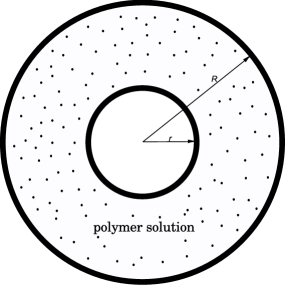
Figure 1:

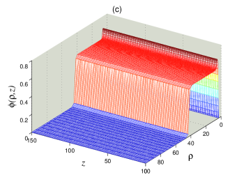
Figure 2: