Weighted Trade Network in a Model of Preferential Bipartite Transactions

Abstract

Using a model of wealth distribution where traders are characterized by quenched random saving propensities and trade among themselves by bipartite transactions, we mimic the enhanced rates of trading of the rich by introducing the preferential selection rule using a pair of continuously tunable parameters. The bipartite trading defines a growing trade network of traders linked by their mutual trade relationships. With the preferential selection rule this network appears to be highly heterogeneous characterized by the scale-free nodal degree and the link weight distributions and presents signatures of non-trivial strength-degree correlations. With detailed numerical simulations and using finite-size scaling analysis we present evidence that the associated critical exponents are continuous functions of the tuning parameters. However the wealth distribution has been observed to follow the well-known Pareto law robustly for all positive values of the tuning parameters.

I I Introduction

In a trading society different traders trade among themselves. Thus the wealth distribution of the society dynamically evolves through this trading process. In the simplest possible situation pairs of traders make economic transactions. Such a mutual interaction can be looked upon establishing a connection between them. Consequently one can define a trade network where each trader is a node and a link is established between a pair of nodes when the corresponding traders make a mutual trading. In this paper we study the growth and the structural properties of a trade network in the framework of a well known model of wealth distribution, namely the Kinetic Exchange Model (KEM) with quenched random saving propensities Yakovenkoreview ; ACandBKC .

Over the last decade tremendous amount of research efforts have been devoted to study the structures, properties and functions of different real-world as well as theoretically defined model networks Vesp . The key characteristic features of these networks include their small-world properties, which simply implies the existence of a very short global connectivity even when the sizes of the networks are extremely large Watts . Secondly, there are a large class of networks that are extremely heterogeneous. Their heterogeneity are quantified by their degree (number of links meeting at a node) distributions. Usually such networks are observed to have power law decay of their degree distributions and are called Scale-free Networks Bara . It has also been apparent that the links of many of these networks appear with a wide variation of strengths. In graph theoretic language the link strengths are called the ‘weights’ in general. Such weighted networks have also been studied in the context of the passenger traffics of airport networks Guimera ; Barrat , international trade networks (ITN) etc. Serrano ; ITN .

More than a century ago Pareto proposed that the distribution of wealth $x$ in a society to be ${\rm P}(x)\sim x^{-(\nu+1)}$ Pareto . This form of distribution is generally known as Pareto distribution for a value of $\nu\sim 1$ Wikipedia . Pareto suggested that $\nu=1$ for the wealth distribution and it is known as the Pareto law.

Application of the concepts of Statistical Physics to the wealth/income distribution in a society goes back to 1931 when Saha and Srivastava had suggested that the form of the wealth distribution may be similar to the Maxwell-Boltzmann distribution of molecular speeds in an ideal gas Saha ; Sinha . Over the last few years renewed attempts have been made using Statistical Physics methods. The main objective is to reproduce the recently collected individual income tax data in different countries reflecting the wealth distributions. It has been observed that these data fit well to exponentially decaying functions for small wealths which however ends with power law tails in the large wealth regime.

Drăgulescu and Yakovenko (DY) DY modeled a bipartite trading between two traders using the analogy of a pair of gas molecules interacting through an energy conserved elastic collision in an ideal gas. Starting from an arbitrary distribution of individual wealths the system evolves through a series of bipartite trades to arrive at a stationary state where the wealth distribution assumes its time independent form. While the DY model produces only an exponentially decaying wealth distribution, later modifications were suggested for its improvement. This class of models are now referred as the KEMs Yakovenkoreview ; ACandBKC .

In a KEM the society is considered as a collection of $N$ traders, each having a certain amount of money equivalent to his wealth $x_{i},\{i=1,N\}$ which he uses for mutual trades with other traders. Generally all traders are initially given an equal amount of money ${\rm P}(x_{i},t=0)=\delta(x_{i}-a)$. The sequential time $t$ is the number of bipartite trades. A trade consists of two parts, (i) a rule for the selection of a distinct pair of traders $i$ and $j$, $(i\neq j)$ and (ii) a distribution rule for the random shuffling of their total money $x_{i}+x_{j}$ between them. Different KEMs differ from one another either in the selection rule or in the distribution rule or in both. In the DY model a pair of traders is selected with uniform probability. Their total money is then randomly reshuffled between them. In the stationary state the wealth distribution is ${\rm P}(x)=\exp(-x/\langle x\rangle)/\langle x\rangle$ where the mean wealth $\langle x\rangle=a$ is usually set at unity DY . Quite naturally a trader invests a only a part of his money in a trade and not his entire wealth. To incorporate this fact Chakraborti and Chakrabarti (CC) introduced a saving propensity $\lambda$ CC same for all traders. As a result the stationary state wealth distribution gets modified to a distribution with a single maximum which approximately fits to a Gamma distribution Patriarca .

In a second modification of the DY model Chatterjee, Chakrabarti and Manna (CCM) assigned a quenched distribution of saving propensities $\{\lambda_{i}\}$ so that each trader is characterized by his own $\lambda_{i}$ value CCM . Using the same selection rule as in DY model, the total money invested by a pair of traders after saving has been randomly shared between them. The system reaches a stationary state here as well but it sensitively depends on the precise values of $\lambda_{i}$s. The wealth distribution in the stationary state after averaging over different realizations of the quenched disorder $\{\lambda_{i}\}$ yields a power law decay with a value of the Pareto exponent $\nu\approx 1$ CCM . However, subsequent detailed analyses have revealed that the CCM model has many interesting features Kunal . For example, in contrast to the DY and CC models, CCM model is not ergodic. Therefore the wealth distribution is not self-averaging and the single trader wealth distribution is totally different from the over all wealth distribution of the whole society. Consequently the individual saving propensity factor $\lambda_{i}$ plays the role of an identification label that determines the economic strength of a member in the society Kunal . In fact, the wealth of a trader fluctuates around a mean value which depends very sensitively on the precise value of $\lambda_{i}$. Larger the value of $\lambda$ higher is the mean wealth. Truly the wealth distribution averaged over many uncorrelated quenched $\{\lambda_{i}\}$ sets is the convolution of the individual members’ wealth distributions Kunal . This overall distribution for the whole system exhibits Pareto law but not the individual member distributions. The exponent $\nu=1$ has been found to be exactly equal to unity in Mohanty ; BasuMohanty .

In section II we describe our modification of the CCM model using the preferential selection rule. The wealth distribution of the modified CCM model has been described in section III. In section IV we define the associated trade network in terms of its nodal degrees and link weights. Section V presents the degree distribution and the weight distribution is discussed in section VI. We summarize in section VII.

II II The Model

It is a general observation that in a society the rich traders invest much more in trade and therefore take part in the trading process more frequently than the poor ones. To incorporate this fact in the CCM model that rich traders are preferentially selected more frequently with higher probabilities we introduce two parameters $\alpha$ and $\beta$ in general, both $\geq 0$, to tune the preference different traders receive for their selections. We assume that the probability of selection of a trader is directly proportional to the $\alpha$ and $\beta$-th power of its wealth. Therefore a pair of traders $i$ and $j$ $(i\neq j)$ with money $x_{i}$ and $x_{j}$ are selected with probabilities

$$\pi_{i}(t)\propto x_{i}(t)^{\alpha}{\hskip 28.45274pt}{\rm and}{\hskip 28.45274pt}\pi_{j}(t)\propto x_{j}(t)^{\beta}.$$ (1)

When $\alpha=\beta=0$ we get the ordinary CCM. When they are non-zero the rich traders are selected with larger probabilities. More rich a trader, higher is the probability that it will be selected for trading. Once a pair of traders $i$ and $j$ is selected, they save $\lambda_{i}$ and $\lambda_{j}$ fractions of their money and invest the rest amounts to the mutual trade. The total invested amount by both the traders is therefore

$$\delta_{ij}(t)=\bar{\lambda}_{i}x_{i}(t)+\bar{\lambda}_{j}x_{j}(t),$$ (2)

where $\bar{\lambda}=1-\lambda$. This amount is then randomly divided into two parts and received by them randomly:

$$x_{i}(t+1)=\lambda_{i}x_{i}(t)+\epsilon(t)\delta_{ij}(t)$$

$$x_{j}(t+1)=\lambda_{j}x_{j}(t)+\bar{\epsilon}(t)\delta_{ij}(t).$$ (3)

where $\epsilon(t)$ is a freshly generated random fraction and $\bar{\epsilon}=1-\epsilon$.

It is essential that all measurements are done once the system attains the stationary state. For that it is necessary that a number of transactions take place between every pair of traders, only then the mean wealths of traders attain their stationary values and fluctuate around them. Eqn. (1) states that for any $(\alpha,\beta)>0$ the richest and the next rich are the most probable pair and the poorest and the next poor are the least probable pair for selection. Assuming the maximum wealth $x_{max}\sim N$ (with $\langle x\rangle$=1) and the minimal wealth $x_{min}\sim 1/N$ the relaxation time can be estimated which is the typical time required for the poorest pair to make a trade. The poorest is selected with a probability $x^{\alpha}_{min}/\Sigma_{i}x^{\alpha}_{i}$. Approximating the denominator by its maximum value we get $(x_{min}/x_{max})^{\alpha}\sim N^{-2\alpha}$. Similarly the probability for the next poorest is $N^{-2\beta}$ and for the poorest pair as $N^{-2(\alpha+\beta)}$. Therefore the time required for a trade between the poorest pair $T_{2}\sim N^{2(\alpha+\beta)}$ (see below) and the relaxation time is several multiples of $T_{2}$. Thus for any $(\alpha,\beta)>0$ the relaxation time grows very rapidly with $N$.

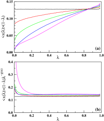
Figure 1: (Color online) (a) Plots of $\langle x(\lambda)\rangle(1-\lambda)$ vs. $\lambda$ for $\alpha=\beta=0$ (black), 1/2 (red), 1 (green), 3/2 (blue) and 2 (magenta) for $N$ = 1204 ($\alpha$ increases from top to bottom). (b) The product function $\langle x(\lambda)\rangle(1-\lambda)\lambda^{-\chi(\alpha)}$ is plotted with $\lambda$ using $\chi(\alpha)$ = 0.15, 0.35, 0.57 and 0.80 for $\alpha$ = 1/2, 1, 3/2 and 2 respectively using the same colors as in (a).

At the early stage rich traders at the top level quickly take part in the trading but gradually the inclusion of relatively poor traders becomes increasingly slower. As a result the number of distinct traders taking part in the trading process grows very slowly. Effectively this implies that the system passes through a very slow transient phase which is practically time independent. We call this state as the “quasi-stationary state (QSS)”. It is to be noted that in the following sections we present our numerical results for large system sizes in the QSS only. To ensure that the system has indeed reached the QSS in our simulations we keep track of the quantity $\Sigma_{i}x^{2}_{i}$ and collect the data only after no appreciable change of its mean value is noticed. We mostly analyse the symmetric $\alpha=\beta$ cases except for a few asymmetric cases.

III III Wealth Distribution

For CCM it was observed that the average money of a trader $\langle x(\lambda)\rangle$ with saving propensity $\lambda$ diverges as $\lambda\to 1$ Kunal . Later it was shown that the divergence is like $\langle x_{i}\rangle(1-\lambda_{i})=$ constant Patriarca1 ; Mohanty . This is simply because had there been a trader with $\lambda=1$, he would not invest any money at all but always receives a share of the investments of the other traders! As a result this trader will eventually grab all the money of the society and, and this situation is similar to the phenomenon of condensation.

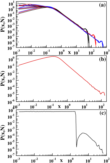
Figure 2: (Color online) (a) Wealth distribution $P(x,N)$ vs. $x$ for $\alpha=\beta$ = 0, 1/2, 1 and 2 and for $N$ = 256 (black), 1024 (red) and 4096 (blue) ($N$ increases from left to right). The slopes of these curves yield $\nu=1.00(3)$ consistent with the Pareto law. (b) $P(x,N)$ for $(\alpha,\beta)=(\infty,0)$ (black) and $(0,\infty)$ (red) for $N$= 1024 which almost overlapped. (c) $P(x,N)$ for $(\alpha,\beta)=(\infty,\infty)$, the distribution is uniform followed by a hump due to transactions between the richest and the next richest traders only.

In Fig. 1(a) we plot the quantity $\langle x(\lambda)\rangle(1-\lambda)$ vs. $\lambda$ for five different values of $\alpha=\beta$ = 0, 1/2, 1, 3/2 and 2. For $\alpha=\beta=0$ we see the horizontal line as observed in Patriarca1 . However for other $\alpha,\beta$ values the variations of the same quantity are far from being uniform and are monotonically increasing with $\lambda$, their growth becoming increasingly faster with $\alpha$. Therefore we try multiplying this function by $\lambda^{-\chi(\alpha)}$ where $\chi(\alpha)$ is a function of the parameter $\alpha$. In Fig. 1(b) we plot $\langle x(\lambda)\rangle(1-\lambda)\lambda^{-\chi(\alpha)}$ vs. $\lambda$ using the same data of Fig. 1(a) using $\chi(\alpha)=$ 0.15, 0.35, 0.57 and 0.80 for $\alpha=\beta=$ 1/2, 1, 3/2 and 2 respectively. We get nearly uniform variations between $\lambda=0.3$ and 1. We assume that

$$\langle x(\lambda)\rangle(1-\lambda)\lambda^{-\chi(\alpha)}=constant.$$ (4)

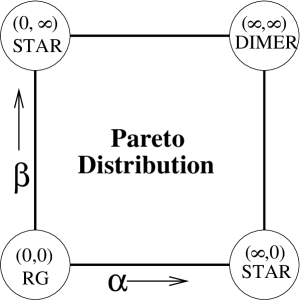
Figure 3: The phase diagram in the positive quadrant of the $(\alpha,\beta)$ plane. The Pareto law is valid in the entire region. The origin corresponds to the CCM model where the trade network is a random graph. At the corners $(\infty,0)$ and $(0,\infty)$ the richest trader trade in every transaction, so that the network is a star-like graph but the wealth distribution still follows Pareto law as shown in Fig. 2(b). However at the corner $(\infty,\infty)$ the trade takes place between the top two richest traders and the network shrinks to a single dimer. The wealth distribution here is uniform followed by a hump as shown in Fig. 2(c).

If the distribution of $\lambda$ values is denoted by $g(\lambda)=constant$, and since the wealth $x$ and the saving propensity $\lambda$ are the two mutually dependent variables associated with the same trader, their probability distributions follow the relation Mohanty

$$P(x)dx=g(\lambda)d\lambda.$$ (5)

Differentiating Eqn. (4) with $\lambda$ one can find out the derivative $d\lambda/dx$ and substituting in Eqn. (5) one gets

$$P(x)=\frac{C}{x^{2}}[\lambda^{-\chi}+(1-\lambda)\chi\lambda^{-\chi-1}]^{-1}.$$ (6)

For this equation we see that for large $\lambda$ the term within $[..]$ is of the order of unity. Therefore in this range $P(x)\sim x^{-2}$ as in the Pareto law. This is an indication that even for $(\alpha,\beta)>0$, Pareto law holds good and in the following we present numerical evidence in support of that.

The system is prepared by assigning uniformly distributed random fractions for the saving propensities $\lambda_{i}$ to all $N$ traders. Here $\lambda_{i}$s are quenched variables and therefore they remain fixed during the subsequent time evolution of the trading system. Consequently all observable that we measured are averaged over different uncorrelated sets of the $\{\lambda_{i}\}$ values. While assigning the $\lambda$ values we first draw $N$ uniformly distributed random fractions, but then to avoid the situation when $\lambda_{max}$ is very close to unity by chance we scale them proportionately so that $\lambda_{max}=1-1/N$ in every $\{\lambda_{i}\}$ set. First a pair of values for ($\alpha,\beta$) is selected. Two types of initial wealth distributions are used: (i) $x_{i}=1$ for all $i$ and (ii) $x_{i}$s are uniformly distributed random numbers with $\langle x\rangle$ = constant. The sequence of bipartite trading begins by randomly selecting pairs of traders using Eqn. 1. Once a pair is selected, their total individual invested amount $\delta_{ij}$ is calculated using Eqn. 2 and this amount is shared again between them using Eqn. 3. This constitute a single bipartite trading and the dynamics is followed over a large number of such trading events.

The wealth distribution changes with time from the initial distribution to more and more flat distribution. After a certain time the system passes through the quasi stationary state when no appreciable change in the wealth distribution is observed. It is also observed that the distribution is robust with respect to the precise values of the parameters $\alpha$ and $\beta$ used. In Fig. 2(a) the wealth distribution $P(x,N)$ has been plotted with $x$ for four sets of parameter values namely, $\alpha=\beta$ = 0, 1/2, 1 and 3/2 and for three system sizes $N$ = 256, 1024 and 4096. Apart from slight fluctuations the four curves for a given system size nearly overlap on one another. On a double logarithmic scale the slopes of the curves give an average estimate for $\nu=1.00(3)$ consistent with the Pareto law as observed in the CCM CCM . This indicates that the wealth distribution is robust with respect to the parameter values in this region. The non-zero values of $\alpha$ and $\beta$ only controls the frequencies with which different traders are called for trading.

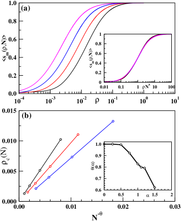
Figure 4: (Color online) Growth of the trade network. (a) Plot of the average size of the giant component $\langle s_{m}(\rho,N)\rangle$ with the link density $\rho$, for $\alpha=\beta=1$ and for $N$ = 128 (black), 256 (red), 512 (blue) and 1024 (pink), ($N$ increases from right to left). The inset shows a data collapse of the same plots with $\rho N^{\theta}$, and ${\theta}=0.88$. (b) The percolation link density $\rho_{c}(N)$ is plotted with $N^{-\theta}$ where $\theta$ = 0.88, 0.92 and 1 for $\alpha=\beta=1/2,3/4$ and 1 respectively. The inset plots $\theta(\alpha)$ with $\alpha$.

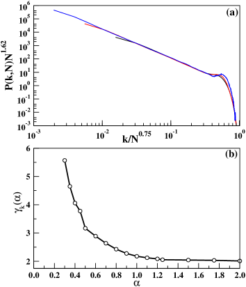
Figure 5: (Color online) (a) The finite-size scaling of the degree distributions $P(k,N)$ for $\alpha=\beta=1$, for $N$ = 256 (black), 1024 (red) and 4096 (blue), and for $\langle k\rangle$ = 1. Direct measurement of slopes give $\gamma_{k}(1)=2.18(3)$. The best data collapse corresponds to $\eta_{k}(1)=1.62$ and $\zeta_{k}(1)=0.75$ giving $\gamma_{k}(1)=2.16(3)$. (b) The plot of $\gamma_{k}(\alpha)$ vs. $\alpha$.

Next we consider the case when one of the two parameters $(\alpha,\beta)$ is infinity and the other one is zero. If $\alpha=\infty$ the richest trader is always selected as the first trader. The other trader is selected among the other $N-1$ traders with uniform probability. As shown in Fig. 2(b) here also we see that the Pareto law holds good. For $\alpha=\infty$ and for finite $\beta$ first the richest trader is selected and then the second trader is selected with probability $\propto x_{j}^{\beta}$. We observe numerically that here also Pareto law works very well.

However the situation is very different when both $(\alpha,\beta)$ take very large values. In this situation almost always only the rich traders are called for transactions. The system passes through an extremely long QSS and the number of traders taking part in trade does not increase at all. For example in the limiting case of $(\alpha,\beta)$ = $(\infty,\infty)$ it implies that always only the richest and the next richest traders are selected for transactions with probability one but not any other trader. If their wealths are very high then the trading will be limited only between them. Therefore the wealth distribution for the single ${\lambda_{i}}$ set has two very high peaks and wealths of all other traders are small and uniformly distributed. Consequently the quench averaged wealth distribution is uniform throughout followed by a hump at the highest value of wealth (Fig. 2(c)). A systematic analysis with many different $(\alpha,\beta)$ pairs leads us to conclude that Pareto law holds good in the positive quadrant of the entire $(\alpha,\beta)$ plane.

In Fig. 3 we exhibit this behavior in the positive quadrant of the $(\alpha,\beta)$ plane where Pareto law is valid and the limiting points are marked by circles with their characteristics. The origin at $(\alpha=0,\beta=0)$ represents the CCM model where traders are selected randomly with uniform probabilities. As explained below, the trade network corresponding to this point is a random graph (RG). As explained before that at the two corners $(\infty,0)$ and $(0,\infty)$ the richest trader always participates in every transaction. Therefore the corresponding trade networks have star-like structures. In the last corner of $(\infty,\infty)$ the trade takes place only between the richest and the next rich traders and therefore the graph reduced to a single dimer only.

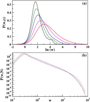
Figure 6: (Color online) Probability distribution $P(w,\alpha)$ of the link weights. (a) Plots for the $N$-clique graphs with $N$ =64 and for $\alpha$= 0 (black), 1/4 (green), 1/2 (blue), 3/4 (magenta) and 1 (red) and $\beta$ =1 always. (b) Plots for $\langle k\rangle$ = 5 with $\alpha=\beta=1$ and for the system sizes 128 (black), 256 (red) and 512 (blue). Direct measurement of slopes gives 2.52, 2.53 and 2.51 respectively.

IV IV The Trade Network

One can associate a network with this trading system. Each trader is a node of the network. Initially the network has only $N$ nodes but no links. First the system is allowed to reach the QSS and then the network starts growing. Every time a pair of traders makes a trade for the first time, a link is introduced between their nodes. There after no further link is added between them irrespective of their subsequent trades and they remain connected with a single link. As the system evolves more and more new traders take part in the trading dynamics and consequently the number of links grow in the network. For $\alpha=\beta=0$ the growth of the network is exactly the same as that of the random graph, however it is much different when $(\alpha,\beta)>0$. Since the rich nodes are preferentially selected they acquire links at a faster rate than the poor nodes. The degree $k_{i}$ of the node $i$ is the number of distinct traders with whom the $i$-th trader has ever traded. The dynamics is continued for a certain time $T$ till the average degree $\langle k\rangle$ of a node reaches a specific pre-assigned value.

In general there are two characteristic time scales involved. At the early stage the network grows with multiple components with different sizes. At time $T_{1}$ the growing network becomes a single component connected graph. A second time scale is $T_{2}$ when the whole network is a $N$-clique graph in which each node is linked to all others, which means each trader has traded at least once with all others. Unlike random graphs the growth of the network is highly heterogeneous and the rich traders have much larger degrees than the poor traders. Since poor traders are selected with low probabilities they take much longer times to be a part of the network. Consequently $T_{1}$ is found to be very large and of the same order as $T_{2}$. Numerically it is easier to calculate $T_{2}$, one keeps track of the number of distinct links and stops only when this number becomes just equal to $[N(N-1)]/2$. On the other hand to calculate $T_{1}$ one follows the growth of the giant component and stops when the giant component covers all $N$ nodes. A Hoshen-Kopelman cluster counting algorithm Hoshen is used to estimate the size of the giant component. For the ordinary CCM with $\alpha=\beta=0$ since both traders are chosen with uniform probability, the generated graph is a simple Erdős-Rényi random graph characterized by a Poissonian degree distribution Erdos .

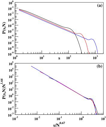
Figure 7: (Color online) (a) Nodal strength distributions $P(s,N)$ with strength $s$ with $\alpha=\beta=1$, for $N$ = 256, 1024 and 4096 and for $\langle k\rangle$ = 5. Direct measurement of the slopes of these curves gives $\gamma_{s}=2.50(5)$. (b) The Finite-size scaling analysis of the data in (a) gives $\eta_{s}=1.64$ and $\zeta_{s}=0.67$ estimating the value of $\gamma_{s}=\eta_{s}/\zeta_{s}=2.45(5)$.

The growth of the giant component is studied with increasing number of links $n$ in the in the trade network. The average fraction of nodes in the giant component is denoted by $\langle s_{m}(\rho,N)\rangle$ which is the order parameter in this percolation problem. This has been plotted in Fig. 4(a) using a semi-log scale with link density $\rho=n/[N(N-1)]/2$ in the network. Four curves shown in this figure correspond to $N$ = 128, 256, 512 and 1024 for $\alpha=\beta=1$, the system size increasing from right to left. The inset shows that a data collapse can be obtained by scaling the $\rho$ axis by a factor $N^{\theta}$ with $\theta=0.88$. The critical density of percolation transition $\rho_{c}(N)$ is defined as that particular value of $\rho$ for which the average size of the giant component $\langle s_{m}(\rho,N)\rangle=1/2$. In Fig. 4(b) we show that how the critical percolation threshold $\rho_{c}(N)$ depends on $N$ by plotting it with $N^{-\theta}$ for $\alpha=\beta=$ 1/2, 3/4 and 1. It has been observed that the exponent $\theta(\alpha)$ is dependent on $\alpha$ in general and in the inset of this figure we plot $\theta(\alpha)$ vs. $\alpha$. We see that for $\alpha\leq 1/2$, $x(\alpha)=1$ but for $\alpha>1/2$, $x(\alpha)$ gradually decreases. For Erdős-Rényi random graphs it is known that $x=1$ and therefore this result gives an indication that the trade network seems to be different from random graphs for $\alpha=\beta>1/2$.

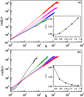
Figure 8: (Color online) (a) Plot of nodal strength $\langle s(k)\rangle$ with degree $k$ for $N=2^{14}$ and for $\alpha=\beta=1/2$ (black), 3/4 (green), 1 (blue), 5/4 (magenta) and 3/2 (red) (from bottom to top). The slopes of these plots estimate $\phi(\alpha)$ shown in the inset. (b) Plot of average wealth $\langle x(k)\rangle$ with degree $k$ for $N=2^{14}$ and for $\alpha=\beta=1/2$ (black), 3/4 (green), 1 (blue), 5/4 (magenta) and 3/2 (red) (from bottom to top). The slopes of these plots estimate $\mu(\alpha)$ shown in the inset.

V V Degree Distribution

The degree distribution has been studied similar to random graphs. We keep track of the average degree $\langle k\rangle$ of the network which is related to the number of links $n$ of the network as $n=\langle k\rangle\frac{N}{2}$. First the degree distribution has been studied for $\langle k\rangle$ = 1 and for different system sizes. For an assigned set of values of $(\alpha,\beta)$, for a given set of values for the saving propensities $\{\lambda_{i}\}$ and for a specific value of $N$ once $\langle k\rangle$ = 1 is reached we calculate the degree distribution considering all components of the network on the same footing. The network is then refreshed by removing all links and a second network is constructed and so on. The dynamics is continued for the same values of the parameters and the same set of $\{\lambda_{i}\}$s till a large number of networks are generated and their mean degree distribution is calculated. The entire dynamical process is then repeated with another uncorrelated set of $\{\lambda_{i}\}$s and the degree distribution has been averaged over many such sets.

In Fig. 5(a) we show the finite-size scaling plot of the average degree distribution $P(k,N)$ vs. $k$ for $\alpha=\beta=1$ and for $N$ = 256, 1024 and 4096. On a double logarithmic scale all three curves show quite long scaling regions followed by humps before the cut-off sizes of the degree distributions. The cut-off sizes of the distributions shifts to the larger values of $k$ approximately by equal amounts on the double-log scale when the system size has been enhanced by the same factor. From the direct measurement of slope in the scaling region we estimate $\gamma(1)=2.18(3)$. Almost the entire degree distribution obeys nicely the usual finite-size scaling analysis and an excellent collapse of the data is observed confirming the validity of the following scaling form:

$$P(k,N)\propto N^{-\eta(\alpha)}{\cal G}[k/N^{\zeta(\alpha)}]$$ (7)

where the scaling function ${\cal G}(y)$ has its usual forms like, ${\cal G}(y)\sim y^{-\gamma(\alpha)}$ as $y\to 0$ and ${\cal G}(y)$ approaches zero very fast for $y>>1$. This is satisfied only when $\gamma(\alpha)=\zeta(\alpha)/\eta(\alpha)$. The exponents $\eta(\alpha)$ and $\zeta(\alpha)$ fully characterize the scaling of $P(k,N)$ in this case. To check the validity of the equation we attempted a data collapse by plotting $P(k,N)N^{\eta(1)}$ vs. $k/N^{\zeta(1)}$ by tuning the values of $\eta(1)$ and $\zeta(1)$. The values obtained for best data collapse are $\eta_{k}(1)=1.62$ and $\zeta_{k}(1)=0.75$ implying that in the infinite size limit $P(k,\infty)\sim k^{-\gamma(1)}$ with $\gamma(1)$ = 2.16(3). Tuning $\alpha$ and $\beta$ to other values it is observed that the degree distribution exponent $\gamma$ does depend on these two parameters. In Fig. 5(b) we show a plot of $\gamma_{k}(\alpha)$ with $\alpha$ which decreases to $\approx 2$ at $\alpha=2$.

VI VI The Weighted Network

Within a certain time $T$ a large number of bipartite trades take place between any arbitrary pair of traders. The total sum of the amounts $\delta_{ij}$ invested in all trades between the traders $i$ and $j$ in time $T$ is defined as the total volume of trade $w_{ij}=\Sigma^{T}\delta_{ij}$. Therefore $w_{ij}$ is regarded as the weight of the link $(ij)$. The magnitudes of weights associated with the links of the trade network are again found to be highly heterogeneous. This is primarily because within a certain time $T$ a rich pair of traders trade many more times than a rich-poor or a poor-poor pair. In addition the invested amounts depend on the mean wealths $\langle x_{i}\rangle$ of the traders involved as well as their saving propensity factors $\lambda_{i}$. The probability distribution $P(w,N)$ of the link weights are calculated when the average degree $\langle k\rangle$ reaches a specific pre-assigned value. As before, this distribution has also been averaged over many weighted networks for one $\{\lambda_{i}\}$ set and then further averaged over many uncorrelated $\{\lambda_{i}\}$ sets.

First we studied the case when the trade networks is a $N$-clique graph, i.e., when each trader has traded with all other traders at least once. Here each node has same degree i.e., $P(k)=\delta(k-(N-1))$ and $\langle k\rangle=N-1$. The required time $T_{2}$ increases rapidly with $N$ as described in section II and we could study small system size $N$ = 64 only. The distribution has a very long tail and therefore we used a lin-log scale for plotting. In Fig. 6(a) we show the plots of $P(w,\alpha)$ with $\ln(w)$ for different values of $\alpha$ = 0, 1/4, 1/2, 3/4 and 1 and $\beta=1$. Each curve is asymmetric and has a single maximum. The position of the peak shifts towards larger values of $\ln(w)$ as $\alpha$ increases. If Fig. 6(b) a similar plot has been shown for $\langle k\rangle=5$ for three network sizes $N$ = 128, 256 and 512 and for $\alpha=\beta=1$. On a double-logarithmic scale each curve has a considerable straight portion. This indicates a power law decay like $P(w,N)\propto w^{-\gamma_{w}}$. The corresponding slopes give estimates for the exponent $\gamma_{w}$ as 2.52, 2.53 and 2.51 for the three system sizes respectively, so that on the average $\gamma_{w}=2.52(3)$.

The strength of a node $s_{i}=\Sigma_{j}w_{ij}$ where $j$ runs over all neighbors $k_{i}$ of $i$, is a measure of the total volume of trade handled by the $i$-th node. Nodal strengths varies over different nodes over a wide range. We first study the probability distribution of nodal strengths. In Fig. 7(a) the strength distribution $P(s,N)$ has been plotted for the average degree $\langle k\rangle=5$, for $\alpha=\beta=1$ and for the network sizes $256,1024$ and 4096. Extended scaling regions at the intermediate regions of the curves indicate that $P(s,N)$ also follows a power-law decay function $P(s,N)\sim s^{-\gamma_{s}}$ in the limit of $N\to\infty$. Direct measurements gives an estimate of $\gamma_{s}(1)\approx 2.5$. In Fig. 7(b) we try a similar finite size scaling of the same data giving $\eta_{s}(1)=1.64$ and $\zeta_{s}(1)=0.67$ giving $\gamma_{s}(1)=2.45(5)$.

Quite often weighted networks have non-linear strength-degree relations reflecting the presence of non-trivial correlations, example of such networks are the airport networks and the international trade network. For a network where the link weights are randomly distributed, the $\langle s(k)\rangle$ grows linearly with $k$. However a non-linear growth like $\langle s(k)\rangle\sim k^{\phi}$ with $\phi>1$, exhibits the presence of non-trivial correlations. In Fig. 8(a) we plot the variation of $\langle s(k)\rangle$ vs. $k$ for a system size $N$ = 16384 and for different values of $\alpha=\beta=1/2$ (black), 3/4 (green), 1 (blue), 5/4 (magenta) and 3/2 (red) (from bottom to top). The slopes of these plots give estimates for the exponent $\phi(\alpha)$ which gradually increased with $\alpha$ and the variation has been plotted in the inset. In the same context we also studied how the mean wealth of a trader depends on its degree. The mean wealth of a trader $\langle x(k)\rangle$ has been plotted in Fig. 8(b) with its degree $k$ for the same system sizes as in Fig. 8(a) and for the same values of parameters. A power law growth has been observed for all values of $\alpha$: $\langle x(k)\rangle\sim k^{\mu(\alpha)}$. The slopes of these plots give estimates for the exponent $\mu(\alpha)$ which has been plotted in the inset of Fig. 8(b).

VII IV Summary

To summarize we have studied the different structural properties of a trade network associated with the dynamical evolution of a model of wealth distribution with quenched saving propensities. In this model distinguishable traders make preferential bipartite trades among themselves and in this way create links. They are selected for trade preferentially using a pair of continuously tunable parameters, where the rich traders are picked up more frequently for trade than poor traders. This creates huge heterogeneity in the system which has been reflected in the power-law distributions of the nodal degree and the link weight distributions measuring the volumes of trade. We present numerical evidence that the associated individual wealth distribution follows the well known Pareto law robustly for all positive values of the parameters.

We thankfully acknowledge P. K. Mohanty, A. Chatterjee and B. K. Chakrabarti for discussion and critical reading of the manuscript.

E-mail: manna@bose.res.in

References

- (1) V. M. Yakovenko and J. Berkley Rosser, arXiv:0905.1518.
- (2) A. Chatterjee and B. K. Chakrabarti, Euro. Phys. Jour. B, 60 135 (2007).
- (3) R. Pastor-Satorras, A. Vespignani, Evolution and Structure of the Internet: A Statistical Physics Approach, Cambridge University Press, Cambridge, 2004.
- (4) D. J. Watts and S.H. Strogatz, Nature 393, 440 (1998).
- (5) A.-L. Barabási and R. Albert, Science, 286, 509 (1999).
- (6) R. Guimera and L. A. N. Amaral, Eur. Phys. Jour. B, 38, 381 (2004).
- (7) A. Barrat, M. Barthélémy, R. Pastor-Satorras, A. Vespignani, Proc. Natl. Acad. Sci. (USA), 101, 3747 (2004).
- (8) M. Á. Serrano and M. Boguñá, Phys. Rev. E. 68, 015101 (2003).
- (9) K. Bhattacharya, G. Mukherjee, J. Saramaki, K. Kaski and S. S. Manna, J. Stat. Mech. P02002 (2008).
- (10) V. Pareto, Cours d’economie Politique (F. Rouge, Lausanne, 1897).
-
(11)
en.wikipedia.org/wiki/Pareto_distribution. - (12) M. N. Saha and B. N. Srivastava, A Treatise on Heat, p105, Indian Press, Allahabad, 1931.
- (13) S. Sinha and B. K. Chakrabarti, Physics News, 39, 33 (2009).
- (14) A. A. Drăgulescu, V. M. Yakovenko, Eur. Phys. J. B 17, 723 (2000).
- (15) A. Chakraborti, B. K. Chakrabarti, Eur. Phys. Jour. B, 17 167 (2000).
- (16) M. Patriarca, A. Chakraborti, K. Kaski, Phys. Rev. E 70, 016104 (2004).
- (17) A. Chatterjee, B. K. Chakrabarti, S. S. Manna, Physica A 335 155 (2004), A. Chatterjee, B. K. Chakrabarti, S. S. Manna, Physica Scripta T 106 36 (2003).
- (18) K. Bhattacharya, G. Mukherjee and S. S. Manna, in Econophysics of Wealth Distributions, (Springer Verlag, Milan, 2005).
- (19) P. K. Mohanty, Phys. Rev. E, 74, 011117 (2006).
- (20) U. Basu and P. K. Mohanty, Eur. Phys. J. B 65, 585 (2008).
- (21) M. Patriarca, A. Chakraborti, K. Kaski, G. Germano, in Econophysics of Wealth Distributions, Eds. A. Chatterjee, S. Yarlagadda, BK Chakrabarti (Springer, Milan, 2005) pp 93-110.
- (22) J. Hoshen and R. Kopelman, Phys. Rev. B, 14, 3428 (1976).
- (23) P. Erdős and A. Rényi, Publ. Math. Debrecen, 6, 290 (1959).