CP Violating Asymmetries
Induced by Supersymmetry
Diplomarbeit
zur Erlangung des akademischen Grades
Diplomingenieur
in der Studienrichtung
Technische Physik
Angefertigt am
Institut für Hochenergiephysik
Österreichische Akademie der Wissenschaften

Betreuung:
Univ. Prof. Dr. Walter Majerotto
Eingereicht von:
Sebastian Frank
Linz, Mai 2008  

Johannes Kepler Universität
A-4040 Linz $\cdot$ Altenbergerstraße 69 $\cdot$ Internet: http://www.jku.at/ $\cdot$ DVR 0093696

 

For Pınar

Eidesstattliche Erklärung

Ich erkläre an Eides statt, daß ich die vorliegende Diplomarbeit selbstständig und ohne fremde Hilfe verfasst, andere als die angegebenen Quellen und Hilfsmittel nicht benutzt bzw. die wörtlich oder sinngemäß entnommenen Stellen als solche kenntlich gemacht habe.

Linz, Mai 2008                                                 Sebastian Frank

Zusammenfassung

Im Minimal Supersymmetrischen Standardmodell (MSSM) mit komplexen Parametern ergeben Einschleifen-Strahlungskorrekturen des Zerfalls eines Stop in ein Bottom-Quark und ein Chargino eine CP verletzende Asymmetrie der Zerfallsbreite

$$\delta^{CP}=\frac{\Gamma^{+}(\tilde{t}_{i}\to b\,\tilde{\chi}^{+}_{k})-\Gamma^{-}(\tilde{t}^{*}_{i}\to\bar{b}\,\tilde{\chi}^{+c}_{k})}{\Gamma^{+}(\tilde{t}_{i}\to b\,\tilde{\chi}^{+}_{k})+\Gamma^{-}(\tilde{t}^{*}_{i}\to\bar{b}\,\tilde{\chi}^{+c}_{k})}\,.$$

Wir führen eine detaillierte, numerische Analyse von $\delta^{CP}$ als auch von $\delta^{CP}\times BR$ (wobei $BR$ das Verzweigungsverhältnis des Zerfalls ist) durch, wobei wir die Abhängigkeit von den beteiligten Parametern und komplexen Phasen untersuchen. Dabei nehmen wir die Yukawa-Kopplungskonstanten des Top- und Bottom-Quarks als laufend an. Wir berücksichtigen die Einschränkungen der Parameter, welche von der experimentellen Obergrenze des elektrischen Dipolmoments des Elektrons ausgehen, indem wir das Dipolmoment während der Analyse automatisch mitberechnen und damit kontrollieren.
Als Resultate erhalten wir für die Asymmetrie $\delta^{CP}$ einen Wert bis zu $\sim 24\,\%$, abhängig vom gewählten Punkt im Parameterraum. Die kombinierte Größe $\delta^{CP}\times\mathrm{BR}$ wird bis zu $\sim 3.5\,\%$ groß.
Wir kommentieren auch die Möglichkeit einer Messung dieser Asymmetrie am Large Hadron Collider (LHC) des CERN. Es wird möglich sein, unsere Asymmetrie der Zerfallsbreite $\delta^{CP}$ am LHC zu messen.

Abstract

In the Minimal Supersymmetric Standard Model (MSSM) with complex parameters, one-loop corrections to the decay of a stop into a bottom-quark and a chargino lead to the CP violating decay rate asymmetry

$$\delta^{CP}=\frac{\Gamma^{+}(\tilde{t}_{i}\to b\,\tilde{\chi}^{+}_{k})-\Gamma^{-}(\tilde{t}^{*}_{i}\to\bar{b}\,\tilde{\chi}^{+c}_{k})}{\Gamma^{+}(\tilde{t}_{i}\to b\,\tilde{\chi}^{+}_{k})+\Gamma^{-}(\tilde{t}^{*}_{i}\to\bar{b}\,\tilde{\chi}^{+c}_{k})}\,.$$

We perform a detailed numerical analysis of $\delta^{CP}$ and also $\delta^{CP}\times BR$ (where $BR$ is the branching ratio of the decay) for $\tilde{t}_{1}\to b\,\tilde{\chi}^{+}_{1}$ and $\tilde{t}_{2}\to b\,\tilde{\chi}^{+}_{1}$, analyzing the dependence on the parameters and complex phases involved. In addition, we take the Yukawa couplings of the top- and bottom-quark running. We account for the constraints on the parameters coming from the experimental limit of the electric dipole moment of the electron by calculating and thus checking it automatically along the way.
We obtain as results that the asymmetry $\delta^{CP}$ rises up to $\sim 24\,\%$, depending on the point in parameter space. The combined quantity $\delta^{CP}\times\mathrm{BR}$ reaches up to $\sim 3.5\,\%$.
We also comment on the feasibility of measuring this asymmetry at the Large Hadron Collider (LHC) at CERN. It will be possible to measure our decay rate asymmetry $\delta^{CP}$ at LHC.

Chapter 1 Introduction

Although the Standard Model (SM) of elementary particle physics is a remarkably successful description of presently known phenomena, it has to be extended to describe physics at high energies properly. Among the theoretical and phenomenological issues that the SM fails to address properly is the baryon asymmetry of the universe [1].
Phenomenologically, there are many reasons to believe that we live in a baryon asymmetric universe, so that there exists much more matter than anti-matter. One strong piece of evidence comes from the acoustic peaks — early universe baryon-photon plasma oscillations — inferred from Cosmic Microwave Background measurements (see e.g. [2]), which give the baryon-to-photon ratio

$$\eta\equiv\frac{n_{B}}{s}\equiv\frac{n_{b}-n_{\bar{b}}}{s}=(6.1^{+0.3}_{-0.2})\times 10^{-10},$$ (1.1)

in which $s$ is the entropy density (roughly the photon density), and $n_{b}$ and $n_{\overline{b}}$ are the number densities of baryons and antibaryons, respectively. This data agrees well with big bang nucleosynthesis, which requires the baryon-to entropy density ratio to be (see e.g. [3, 4])

$$2.6\times 10^{-10}\leq\eta\leq 6.2\times 10^{-10}.$$ (1.2)

The problem of baryogenesis [5] is to explain the origin of this small number starting from the natural initial condition of $\eta=0$, which in most cases is attained at high enough temperatures.
Assuming CPT is preserved, there are three necessary conditions for baryogenesis, usually referred to as the Sakharov requirements [5]:

1. Baryon number violation

2. Departure from thermal equilibrium

3. Charge (C) and Charge-Parity (CP) violation.

Although the Sakharov criteria can be met in the SM, the baryon asymmetry generated at the electroweak phase transition is too small. However, supersymmetric extensions of the SM can contain new sources of CP violation which can increase and thus might explain the baryon asymmetry of the universe.
Supersymmetric models introduce superpartners to every particle, that just differ in the spin quantum number. Since we do not observe such superpartners to the known particles with the same mass, supersymmetry must be broken. This supersymmetry breaking leads to a couple of new parameters. If these parameters are chosen to be complex, supersymmetric models contain new sources of CP violation. In the Minimal Supersymmetric Standard Model (MSSM) — the most promising extension of the SM — the $U(1)$ and $SU(2)$ gaugino (superpartner of gauge bosons) mass parameters $M_{1}$ and $M_{2}$, respectively, the higgsino (superpartner of Higgs-boson) mass parameter $\mu$, as well as the trilinear couplings $A_{f}$ (corresponding to a fermion f) may be complex. Radiative corrections at one-loop level can then lead to new CP violating asymmetries in addition to the small CP asymmetries in the SM coming from the Cabibbo-Kobayashi-Maskawa-(CKM)-matrix.
Although large complex phases are desirable to explain baryogenesis [6, 7, 8, 9], there are constraints on these phases coming from the experimental limits on the electric dipole moments (EDMs) of the electron, neutron and Hg. Especially the complex phase of $\mu$ is highly constrained for a typical SUSY mass scale of the order of a few hundred GeV.
In this thesis we study the CP violating decay rate asymmetry

$$\delta^{CP}=\frac{\Gamma^{+}(\tilde{t}_{i}\to b\,\tilde{\chi}^{+}_{k})-\Gamma^{-}(\tilde{t}^{*}_{i}\to\bar{b}\,\tilde{\chi}^{+c}_{k})}{\Gamma^{+}(\tilde{t}_{i}\to b\,\tilde{\chi}^{+}_{k})+\Gamma^{-}(\tilde{t}^{*}_{i}\to\bar{b}\,\tilde{\chi}^{+c}_{k})}$$ (1.3)

of the decay of a stop (bosonic superpartner of the top-quark) into a bottom-quark and a chargino (mass eigenstate of the superpartners of charged Higgs bosons and charged gauge bosons) in the MSSM with complex parameters at full one-loop level.
The asymmetry is of course zero if CP is conserved and also vanishes at tree-level in the case of CP violation. The complete list of all graphs at one-loop level which contribute to this asymmetry can be found in the Appendix A. They give a contribution only if they have an absorptive part, i.e. at least a second decay channel of $\tilde{t}_{i}$ must be kinematically possible in addition to that into $b\,\tilde{\chi}^{+}_{k}$. In spite of the overall 47 graphs one, however, expects that two graphs will dominate. They are the two possible processes involving a gluino $\tilde{g}$ (see Chapter 9). Because the gluino couples like its superpartner the gluon with the strong interaction force, these contributions are expected to dominate over all others, if the decay channel $\tilde{t}_{i}\to t\,\tilde{g}$ is open ($m_{\tilde{t}_{i}}\geq m_{t}+m_{\tilde{g}}$).
As a loop-level quantity the decay rate asymmetry $\delta^{CP}$ depends on the phases of all complex parameters involved. One, however, expects that the dependence on the phase of $A_{t}$ and $A_{b}$ is strongest (taking $\mu$ real because of the stringent EDM constraints). We neglect the mixing in the neutral Higgs sector due to the complex trilinear couplings of the third generation $(A_{t},A_{b},A_{\tau})$ (see e.g. [10, 11, 12]) because they are very small [13].

We perform a detailed numerical analysis for $\tilde{t}_{1}\to b\,\tilde{\chi}^{+}_{1}$ and $\tilde{t}_{2}\to b\,\tilde{\chi}^{+}_{1}$ analyzing the dependence on the parameters and phases involved. In addition, we take the Yukawa couplings of the top- and bottom-quark running. We account for the constraints coming from the EDM of the electron by calculating and thus checking it automatically along the way. We also comment on the feasibility of measuring this asymmetry at the Large Hadron Collider (LHC) at CERN.
The work is organized as follows:

• In Chapter 2 we give an introduction into the basic concept of supersymmetry (SUSY).

• In Chapter 3 we derive supersymmetric Lagrangians as well as the soft supersymmetry breaking interactions.

• In Chapter 4 we present the particle content of the Minimal Supersymmetric Standard Model (MSSM).

• In Chapter 5 the mass matrices of the sfermions, charginos and neutralinos are derived.

• In Chapter 6 we list the relevant couplings of the most important interactions involved.

• Chapter 7 contains some definitions which are important for the study of CP violating asymmetries.

• Chapter 8 provides a deeper insight into CP violation and the decay rate asymmetry $\delta^{CP}$.

• In Chapter 9 we list the most important processes who are expected to yield the highest $\delta^{CP}$.

• In Chapter 10 we discuss the numerical results and present the conclusions.

• Appendix A holds the complete list of all processes at full one-loop level who can contribute to $\delta^{CP}$.

• In Appendix B we define the Passarino–Veltman integrals and provide them with a special argument set.

• In Appendix C and D we derive a generic structure and a tree-level coupling, respectively.

• Appendix E shows how to transform from Weyl to Dirac spinors and vice versa.

• Finally, in Appendix F we derive the electric dipole moment (EDM) of a fermion and calculate the EDM of the electron.

Chapter 2 Supersymmetry (SUSY)

2.1 Beyond the Standard Model

The Standard Model of elementary particle physics (SM) [14, 15, 16] is a spectacularly successful theory of the known particles and their electroweak and strong forces. The SM is a gauge theory, in which the gauge group $SU(3)_{C}\times SU(2)_{L}\times U(1)_{Y}$ is spontaneously broken to $SU(3)_{C}\times U(1)_{EM}$ by the non-vanishing vacuum expectation value (VEV) of a fundamental scalar field, the Higgs field, at energies of order 100 GeV. Although the SM provides a correct description of all known microphysical non-gravitational phenomena (except neutrino masses and oscillations), there are a number of theoretical and phenomenological issues that the SM fails to address adequately [1]:

• Hierarchy problem. Phenomenologically the mass of the Higgs boson associated with electroweak symmetry breaking must be in the range of $\cal O$(100 GeV). However, radiative corrections to the Higgs mass are quadratically dependent on the ultra-violet cutoff $\Lambda$, since the masses of fundamental scalar fields are not protected by chiral or gauge symmetries. The “natural” value of the Higgs mass is therefore of ${\cal O}(\Lambda)$ rather than $\cal O$(100 GeV), leading to a destabilization of the Higgs mass and the hierarchy of the mass scales in the SM. To achieve $m\sim{\cal O}$(100 GeV) it is necessary to fine-tune the scalar mass-squared parameter $m^{2}_{0}\sim\Lambda^{2}$ of the fundamental ultraviolet theory to a precision of $m^{2}/\Lambda^{2}$. If, for example, $\Lambda=10^{16}$ GeV and $m=100$ GeV, the precision of fine-tuning must be $10^{-28}$, which is very unnatural.

• Electroweak symmetry breaking. In the SM, electroweak symmetry breaking is parameterized by the Higgs boson $h$ and its general potential $V=\mu^{2}|h|^{2}+\lambda|h|^{4}$. In order to make this symmetry breaking happen, one has to set $\mu^{2}<0$ by hand. This postulate is rather artificial.

• Gauge coupling unification. The idea that the gauge couplings undergo renormalization group evolution in such a way that they meet at a point at a high scale lends credence to the picture of grand unified theories (GUTs) and certain string theories. However, precise measurements of the low energy values of the gauge couplings demonstrated that the SM cannot describe gauge coupling unification (see e.g. [17]) accurately enough to imply it is more than an accident.

• Family structure and fermion masses. The SM does not explain the existence of three families and can only parameterize the strongly hierarchical values of the fermion masses. Massive neutrinos imply that the theory has to be extended, as in the SM the neutrinos are strictly left-handed and massless. Right-handed neutrinos can be added, but achieving ultra-light neutrino masses from the seesaw mechanism [18, 19] requires the introduction of a new scale much larger than $\cal O$(100 GeV).

• Cosmological challenges. Several difficulties are encountered when trying to build cosmological models based solely on the SM particle content. As already mentioned in the introduction, the SM cannot explain the baryon asymmetry of the universe. The SM also does not have a viable candidate for the cold dark matter of the universe, nor a viable inflaton. The most difficult problem the SM has when trying to connect with the gravitational sector is the absence of the expected scale of the cosmological constant.

Therefore, the Standard Model must be extended to be valid at higher energies. Theories with low energy supersymmetry have emerged as the strongest candidates for physics beyond the SM. The main idea behind supersymmetry (SUSY) is an underlying symmetry between bosons and fermions. In the simplest supersymmetric world, each SM particle has a superpartner which differs only in the spin by $1/2$ and is related to the original particle by a supersymmetry transformation.
Since no superpartners were discovered yet, SUSY is not an exact symmetry. They seem to have a significant higher mass, which can be explained by spontaneous breaking of the supersymmetry. In other words, the underlying model should have a Lagrangian density that is invariant under supersymmetry, but a vacuum state that is not.

2.2 Predictions and Successes of SUSY

The main reasons that low energy supersymmetry is taken very seriously are not its elegance or its likely theoretical motivations, but its successful explanations and predictions. Of course, these successes may just be remarkable coincidences because there is as yet no direct experimental evidence for SUSY. Superpartners and a light Higgs boson must be discovered or demonstrated not to exist at the Large Hadron Collider (LHC) at CERN. The main successes are as follows [1, 20]:

• Hierarchy problem. SUSY provides a solution to the hierarchy problem by protecting the Higgs mass from large radiative corrections coming from heavy particles. Due to the symmetry between bosons and fermions, each contribution to the radiative correction can be completely canceled in the case of exact SUSY. In the case of broken SUSY the cancelation is not complete but still strong enough to render the corrections to the Higgs mass harmless, if the masses of the new superpartners are $\lesssim{\cal O}$(1 TeV).

• Radiative electroweak symmetry breaking. With plausible boundary conditions at a high scale, low energy supersymmetry can provide the explanation of the origin of electroweak symmetry breaking [21, 22, 23, 24]. To oversimplify a little, the SM effective Higgs potential has the form $V=m^{2}h^{2}+\lambda h^{4}$. First, supersymmetry requires that the quartic coupling $\lambda$ is a function of the $U(1)_{Y}$ and $SU(2)_{C}$ gauge couplings $\lambda=({g^{\prime}}^{2}+g^{2})/2$. Second, the $m^{2}$ parameter runs to negative values at the electroweak scale, driven by the large top quark Yukawa coupling. Thus the “Mexican hat” potential with a minimum away from $h=0$ is derived rather than assumed.

• Gauge coupling unification. In contrast to the SM, the MSSM allows for the unification of the gauge couplings, as first pointed out in the context of GUT models by [25, 26, 27]. The extrapolation of the low energy values of the gauge couplings using renormalization group equations and the MSSM particle content shows that the gauge couplings unify at the scale $M_{G}\simeq 3\times 10^{16}$ GeV [28, 29, 30, 31].

• Cold dark matter. In supersymmetric theories, the lightest superpartner (LSP) can be stable. This stable superpartner provides a nice cold dark matter candidate [32, 33]. Simple estimates of its relic density are of the right order of magnitude to provide the observed amount. LSPs were noticed as good candidates before the need for nonbaryonic cold dark matter was established.

• Supergravity. Gauged SUSY includes a coupling between gravity and matter. The invariance of the Lagrangian density under a local supersymmetry transformation leads to a quantized form of Einstein s general relativity. However, like all known theories that include general relativity, supergravity is still non-renormalizable as a quantum field theory.

• Baryon asymmetry. As already mentioned in the introduction, SUSY may help explain the baryon asymmetry of the universe. At least three different approaches can provide the observed baryon asymmetry: (i) generating the asymmetry at the electroweak phase transition via the electroweak baryogenesis mechanism (see e.g. [9, 8]), (ii) generating it via leptogenesis, and (iii) the Affleck-Dine mechanism [34] using the decay of a scalar field in the early universe into matter. All three mechanism need the existence of CP violation, as the Sakharov criteria demand. The CP violation in the SM is too small to explain baryogenesis, but SUSY can provide sufficient additional sources of CP violation.

Supersymmetry has also made several correct predictions [1]:

• Supersymmetry predicted in the early 1980s that the top quark would be heavy [35, 36], because this was a necessary condition for the validity of the electroweak symmetry breaking explanation.

• Supersymmetric grand unified theories (GUTs) with a high fundamental scale accurately predicted the present experimental value of $\sin^{2}\theta_{W}$ before it was measured [26, 25, 37, 38].

• Supersymmetry requires a light Higgs boson to exist [39, 40], consistent with current precision measurements, which suggest $M_{h}<200$ GeV.

• When the Large Electron-Positron Collider (LEP) began to run in 1989 it was recognized that either LEP would discover superpartners if they were very light or there would be no significant deviations from the SM (all supersymmetry effects at LEP are loop effects and supersymmetry effects decouple as superpartners get heavier). In nonsupersymmetric approaches with strong interactions near the electroweak scale it was natural to expect significant deviations from the SM at LEP.

Together these successes provide a powerful indirect sign that low energy supersymmetry is indeed part of the correct description of nature.
Remarkably, supersymmetry was not invented to explain any of the above physics. Supersymmetry was discovered as a beautiful theory and was studied for its own sake in the early 1970s. Only after several years of studying the theory did it become clear that supersymmetry solved the above problems, one by one. Furthermore, all of the above successes can be achieved simultaneously, with one consistent form of the theory and its parameters. Low energy supersymmetry also has no known incorrect predictions; it is not easy to construct a theory that explains and predicts certain phenomena and has no conflict with other experimental observations.

2.3 The Superalgebra

A supersymmetry transformation turns a bosonic state into a fermionic state, and vice versa [41]. The operator $Q$ that generates such transformations must be an anticommuting spinor with

$$Q|{\rm Boson}\rangle=|{\rm Fermion}\rangle\qquad\qquad Q|{\rm Fermion}\rangle=|{\rm Boson}\rangle\,.$$ (2.1)

Using the Minimal Supersymmetric Standard Model (MSSM), we only deal with a $N=1$ supersymmetry, that means only one generator-pair is needed. Spinors are intrinsically complex objects, so $Q^{\dagger}$ (the hermitian conjugate of $Q$) is also a symmetry generator. Because $Q$ and $Q^{\dagger}$ are fermionic operators, they carry spin angular momentum $1/2$, so it is clear that supersymmetry must be a spacetime symmetry. The possible forms for such symmetries in an interacting quantum field theory are highly restricted by the Haag-Lopuszanski-Sohnius extension of the Coleman-Mandula theorem [42, 43]. For realistic theories like the SM, this theorem implies that the generators $Q$ and $Q^{\dagger}$ must satisfy an algebra of anticommutation and commutation relations with the form

$$\{Q_{\alpha},Q^{\dagger}_{\dot{\alpha}}\}=2\sigma^{\mu}_{\alpha\dot{\alpha}}P_{\mu}\,,$$ (2.2)

$$\{Q_{\alpha},Q_{\beta}\}=\{Q^{\dagger}_{\dot{\alpha}},Q^{\dagger}_{\dot{\beta}}\}=0\,,$$ (2.3)

$$[Q_{\alpha},P^{\mu}]=[Q^{\dagger}_{\dot{\alpha}},P^{\mu}]=0\,$$ (2.4)

where $P^{\mu}$ is the four-momentum generator of spacetime translations, the indices $\alpha,\dot{\alpha}=1,2$ are the left- and right-handed spinor indices and $\sigma$ stands for the Pauli matrices.
The single-particle states of a supersymmetric theory fall into irreducible representations of the supersymmetry algebra, called supermultiplets. Each supermultiplet contains both fermion and boson states, which are commonly known as superpartners of each other. The squared-mass operator $P^{2}$ commutes with the operators $Q$, $Q^{\dagger}$ and with all spacetime rotation and translation operators, so it follows immediately that particles inhabiting the same irreducible supermultiplet must have equal eigenvalues of $P^{2}$, and therefore equal masses. The supersymmetry generators $Q,Q^{\dagger}$ also commute with the generators of gauge transformations. Therefore particles in the same supermultiplet must also be in the same representation of the gauge group, and so must have the same electric charges, weak isospin, and color degrees of freedom.
Each supermultiplet contains an equal number of fermion and boson degrees of freedom. There are in total two different types of supermultiplets possible. The so called chiral supermultiplet includes a two-component spin-$1/2$ Weyl fermion and a complex spin-$0$ field, whereas the gauge supermultiplet combines a spin-$1/2$ gaugino (the fermionic superpartner of a gauge boson) and a spin-$1$ gauge boson.
In a supersymmetric extension of the SM, each of the known fundamental particles is thus in either a chiral or a gauge supermultiplet, and must have a superpartner with spin differing by $1/2$ unit. What remains is to decide exactly how the known particles fit into the supermultiplets, and to give them appropriate names. This will be done in Chapter 4, but first we want to introduce the supersymmetric Lagrangian density and the (soft) SUSY breaking terms.

Chapter 3 Supersymmetric Lagrangians

In this chapter we will describe the construction of supersymmetric Lagrangians and soft supersymmetry breaking terms [41, 20]. We can then apply these results to the special case of the MSSM.

3.1 A Free Chiral Supermultiplet

The simplest supersymmetric model we can build is the massless, non interacting Wess-Zumino model [44], which describes a single chiral supermultiplet, consisting of a left-handed two-component Weyl fermion $\psi$ and its superpartner, a complex scalar field $\phi$. The simplest action we can write down is

$$S = \int d^{4}x\>\left(\mathcal{L}_{\rm scalar}+\mathcal{L}_{\rm fermion}\right)\,,$$ (3.1)

$$\mathcal{L}_{\rm scalar} = \partial^{\mu}\phi^{*}\partial_{\mu}\phi\,,$$ (3.2)

$$\mathcal{L}_{\rm fermion} = i\psi^{\dagger}\bar{\sigma}^{\mu}\partial_{\mu}\psi\,.$$ (3.3)

A supersymmetry transformation should turn the scalar boson field $\phi$ into something involving the fermion field $\psi_{\alpha}$. The simplest possibility for the transformation of the scalar field is

$$\delta\phi=\epsilon\psi\,,\qquad\qquad\delta\phi^{*}=\epsilon^{\dagger}\psi^{\dagger}\,,$$ (3.4)

where $\epsilon^{\alpha}$ is an infinitesimal, anticommuting, two-component Weyl fermion object parameterizing the supersymmetry transformation. As we only discuss global supersymmetry, $\epsilon^{\alpha}$ is a constant, satisfying $\partial_{\mu}\epsilon^{\alpha}=0$. The scalar part of the lagrangian now transforms as

$$\delta\mathcal{L}_{\rm scalar}=\epsilon\partial^{\mu}\psi\>\partial_{\mu}\phi^{*}+\epsilon^{\dagger}\partial^{\mu}\psi^{\dagger}\>\partial_{\mu}\phi\,.$$ (3.5)

We would like for this to be canceled by $\delta\mathcal{L}_{\rm fermion}$, at least up to a total derivative, so that the action will be invariant under the supersymmetry transformation. This leads to only one possibility (up to a multiplicative constant):

$$\delta\psi_{\alpha}=-i(\sigma^{\mu}\epsilon^{\dagger})_{\alpha}\>\partial_{\mu}\phi\,,\qquad\qquad\delta\psi^{\dagger}_{\dot{\alpha}}=i(\epsilon\sigma^{\mu})_{\dot{\alpha}}\>\partial_{\mu}\phi^{*}\,.$$ (3.6)

With this guess, one immediately obtains

$$\delta\mathcal{L}_{\rm fermion}=-\epsilon\sigma^{\mu}\bar{\sigma}^{\nu}\partial_{\nu}\psi\>\partial_{\mu}\phi^{*}+\psi^{\dagger}\bar{\sigma}^{\nu}\sigma^{\mu}\epsilon^{\dagger}\>\partial_{\mu}\partial_{\nu}\phi\,.$$ (3.7)

After applying the Pauli matrix identities

$$\bigl{[}\sigma^{\mu}\bar{\sigma}^{\nu}+\sigma^{\nu}\bar{\sigma}^{\mu}\bigr{]}_{\alpha}{}^{\beta}=2\eta^{\mu\nu}\delta_{\alpha}^{\beta}\,,\qquad\bigl{[}\bar{\sigma}^{\mu}\sigma^{\nu}+\bar{\sigma}^{\nu}\sigma^{\mu}\bigr{]}^{\dot{\beta}}{}_{\dot{\alpha}}=2\eta^{\mu\nu}\delta_{\dot{\alpha}}^{\dot{\beta}}\,,$$ (3.8)

and using the fact that partial derivatives commute $(\partial_{\mu}\partial_{\nu}=\partial_{\nu}\partial_{\mu})$, it takes the form

$$\delta\mathcal{L}_{\rm fermion} = -\epsilon\partial^{\mu}\psi\>\partial_{\mu}\phi^{*}-\epsilon^{\dagger}\partial^{\mu}\psi^{\dagger}\>\partial_{\mu}\phi$$ (3.9)

$$-\partial_{\mu}\left(\epsilon\sigma^{\nu}\bar{\sigma}^{\mu}\psi\>\partial_{\nu}\phi^{*}-\epsilon\psi\>\partial^{\mu}\phi^{*}-\epsilon^{\dagger}\psi^{\dagger}\>\partial^{\mu}\phi\right)\,.$$

The first two terms here just cancel against $\delta\mathcal{L}_{\rm scalar}$, while the remaining contribution is a total derivative. So we arrive at

$$\delta S=\int d^{4}x\>\>\,(\delta\mathcal{L}_{\rm scalar}+\delta\mathcal{L}_{\rm fermion})=0\,,$$ (3.10)

justifying our guess of the numerical multiplicative factor made in Eq. (3.6).
We must also show that the supersymmetry algebra closes; in other words, that the commutator of two supersymmetry transformations parameterized by two different spinors $\epsilon_{1}$ and $\epsilon_{2}$ is another symmetry of the theory. Using Eq. (3.6) in Eq. (3.4) one finds

$$(\delta_{\epsilon_{2}}\delta_{\epsilon_{1}}-\delta_{\epsilon_{1}}\delta_{\epsilon_{2}})\phi\,\equiv\,\delta_{\epsilon_{2}}(\delta_{\epsilon_{1}}\phi)-\delta_{\epsilon_{1}}(\delta_{\epsilon_{2}}\phi)=-i(\epsilon_{1}\sigma^{\mu}\epsilon_{2}^{\dagger}-\epsilon_{2}\sigma^{\mu}\epsilon_{1}^{\dagger})\>\partial_{\mu}\phi\,.$$ (3.11)

We have found that the commutator of two supersymmetry transformations gives us back the derivative of the original field. Since $\partial_{\mu}$ corresponds to the generator of spacetime translations $P_{\mu}$, this equation implies the form of the supersymmetry algebra that was foreshadowed in Eq. (2.2).
For the fermion $\psi$ the commutator takes the form

$$(\delta_{\epsilon_{2}}\delta_{\epsilon_{1}}-\delta_{\epsilon_{1}}\delta_{\epsilon_{2}})\psi_{\alpha}=-i(\sigma^{\mu}\epsilon_{1}^{\dagger})_{\alpha}\>\epsilon_{2}\partial_{\mu}\psi+i(\sigma^{\mu}\epsilon_{2}^{\dagger})_{\alpha}\>\epsilon_{1}\partial_{\mu}\psi\,.$$ (3.12)

After applying the Fierz identity

$$\chi_{\alpha}\>(\xi\eta)=-\xi_{\alpha}\>(\eta\chi)-\eta_{\alpha}\>(\chi\xi)$$ (3.13)

with $\chi=\sigma^{\mu}\epsilon_{1}^{\dagger}$, $\xi=\epsilon_{2}$, $\eta=\partial_{\mu}\psi$, and again with $\chi=\sigma^{\mu}\epsilon_{2}^{\dagger}$, $\xi=\epsilon_{1}$, $\eta=\partial_{\mu}\psi$, followed in each case by an application of the identity

$$\xi^{\dagger}\bar{\sigma}^{\mu}\chi=-\chi\sigma^{\mu}\xi^{\dagger}=(\chi^{\dagger}\bar{\sigma}^{\mu}\xi)^{*}=-(\xi\sigma^{\mu}\chi^{\dagger})^{*}$$ (3.14)

we obtain

$$(\delta_{\epsilon_{2}}\delta_{\epsilon_{1}}-\delta_{\epsilon_{1}}\delta_{\epsilon_{2}})\psi_{\alpha}=-i(\epsilon_{1}\sigma^{\mu}\epsilon_{2}^{\dagger}-\epsilon_{2}\sigma^{\mu}\epsilon_{1}^{\dagger})\>\partial_{\mu}\psi_{\alpha}+i\epsilon_{1\alpha}\>\epsilon_{2}^{\dagger}\bar{\sigma}^{\mu}\partial_{\mu}\psi-i\epsilon_{2\alpha}\>\epsilon_{1}^{\dagger}\bar{\sigma}^{\mu}\partial_{\mu}\psi\,.$$ (3.15)

The last two terms vanish on-shell; that is, if the equation of motion $\bar{\sigma}^{\mu}\partial_{\mu}\psi=0$ following from the action is enforced. The remaining piece is exactly the same spacetime translation that we found for the scalar field. The fact that the supersymmetry algebra only closes on-shell (when the classical equations of motion are satisfied) might be somewhat worrisome, since we would like the symmetry to hold even quantum mechanically. This can be fixed by a trick. We invent a new complex scalar field $F$, which does not have a kinetic term. Such fields are called auxiliary, and they are really just book-keeping devices that allow the symmetry algebra to close off-shell. The Lagrangian density for $F$ and its complex conjugate is simply

$$\mathcal{L}_{\rm auxiliary}=F^{*}F$$ (3.16)

which leads to the equations of motion $F=F^{*}=0$. The new field is now included in the supersymmetry transformation rules

$$\delta F=-i\epsilon^{\dagger}\bar{\sigma}^{\mu}\partial_{\mu}\psi\,,\qquad\qquad\delta F^{*}=i\partial_{\mu}\psi^{\dagger}\bar{\sigma}^{\mu}\epsilon\,.$$ (3.17)

Now the auxiliary part of the Lagrangian density transforms as

$$\delta\mathcal{L}_{\rm auxiliary}=-i\epsilon^{\dagger}\bar{\sigma}^{\mu}\partial_{\mu}\psi\>F^{*}+i\partial_{\mu}\psi^{\dagger}\bar{\sigma}^{\mu}\epsilon\>F$$ (3.18)

which vanishes on-shell, but not for arbitrary off-shell field configurations. By adding an extra term to the transformation law for $\psi$ and $\psi^{\dagger}$

$$\delta\psi_{\alpha}=-i(\sigma^{\mu}\epsilon^{\dagger})_{\alpha}\>\partial_{\mu}\phi+\epsilon_{\alpha}F\,,\qquad\>\>\delta\psi_{\dot{\alpha}}^{\dagger}=i(\epsilon\sigma^{\mu})_{\dot{\alpha}}\>\partial_{\mu}\phi^{*}+\epsilon^{\dagger}_{\dot{\alpha}}F^{*}\,,$$ (3.19)

one obtains an additional contribution to $\delta\mathcal{L}_{\rm fermion}$, which just cancels with $\delta\mathcal{L}_{\rm auxiliary}$, up to a total derivative term. So our “modified” theory with $\mathcal{L}=\mathcal{L}_{\rm scalar}+\mathcal{L}_{\rm fermion}+\mathcal{L}_{\rm auxiliary}$ is still invariant under supersymmetry transformations. Proceeding as before, one now obtains for each of the fields $X=\phi,\phi^{*},\psi,\psi^{\dagger},F,F^{*}$ that the supersymmetry algebra now closes also off-shell

$$(\delta_{\epsilon_{2}}\delta_{\epsilon_{1}}-\delta_{\epsilon_{1}}\delta_{\epsilon_{2}})X=-i(\epsilon_{1}\sigma^{\mu}\epsilon_{2}^{\dagger}-\epsilon_{2}\sigma^{\mu}\epsilon_{1}^{\dagger})\>\partial_{\mu}X\,.$$ (3.20)

The real reason for the necessity to introduce the auxiliary field $F$ is that the two fields $\phi$ and $\psi$ have a different number of degrees of freedom. While on-shell, the two real propagating degrees of freedom of the complex scalar field $\phi$ match with the two spin polarization states of $\psi$, there is a different situation off-shell. Off-shell, the Weyl fermion $\psi$ is a complex two-component object and has four real degrees of freedom (half of the degrees of freedom are eliminated by going on-shell). The difference of degrees of freedom off-shell is corrected by the introduction of two more real scalar degrees of freedom in the complex field $F$, which vanishes going on-shell.
Invariance of the action under a symmetry transformation always implies the existence of a conserved current, and supersymmetry is no exception. The supercurrent $J^{\mu}_{\alpha}$ is an anticommuting four-vector carrying a spinor index. With the Noether procedure we receive

$$\epsilon J^{\mu}+\epsilon^{\dagger}J^{\dagger\mu}\equiv\sum_{X}\,\delta X\>\frac{\delta\mathcal{L}}{\delta(\partial_{\mu}X)}-K^{\mu}$$ (3.21)

where $X=\phi,\phi^{*},\psi,\psi^{\dagger},F,F^{*}$ and $K^{\mu}$ is an object whose divergence is the variation of the Lagrangian density under the supersymmetry transformation, $\delta\mathcal{L}=\partial_{\mu}K^{\mu}$. Calculated explicitly, $J^{\mu}_{\alpha}$ and its hermitian conjugate become

$$J^{\mu}_{\alpha}=(\sigma^{\nu}\bar{\sigma}^{\mu}\psi)_{\alpha}\>\partial_{\nu}\phi^{*}\,,\qquad\qquad J^{\dagger\mu}_{\dot{\alpha}}=(\psi^{\dagger}\bar{\sigma}^{\mu}\sigma^{\nu})_{\dot{\alpha}}\>\partial_{\nu}\phi\,.$$ (3.22)

Using the equations of motion, it can be shown that the supercurrent and its hermitian conjugate are conserved separately:

$$\partial_{\mu}J^{\mu}_{\alpha}=0\,,\qquad\qquad\partial_{\mu}J^{\dagger\mu}_{\dot{\alpha}}=0\,.$$ (3.23)

The corresponding conserved charges to these currents are

$$Q_{\alpha}={\sqrt{2}}\int d^{3}\vec{x}\>J^{0}_{\alpha}\,,\qquad\qquad Q^{\dagger}_{\dot{\alpha}}={\sqrt{2}}\int d^{3}\vec{x}\>J^{\dagger 0}_{\dot{\alpha}}\,.$$ (3.24)

As quantum mechanical operators, they satisfy

$$\left[\epsilon Q+\epsilon^{\dagger}Q^{\dagger},X\right]=-i{\sqrt{2}}\>\delta X$$ (3.25)

for any field $X$, up to terms that vanish on-shell. This further leads (using the canonical equal-time commutation and anticommutation relations) to the supersymmetry algebra

$$\{Q_{\alpha},Q^{\dagger}_{\dot{\alpha}}\}=2\sigma^{\mu}_{\alpha\dot{\alpha}}P_{\mu}\,,\qquad\qquad\{Q_{\alpha},Q_{\beta}\}=\{Q^{\dagger}_{\dot{\alpha}},Q^{\dagger}_{\dot{\beta}}\}=0\,,$$ (3.26)

and since we only deal with global supersymmetry transformations we have

$$[Q_{\alpha},P^{\mu}]=0\,,\qquad\qquad[Q^{\dagger}_{\dot{\alpha}},P^{\mu}]=0\,.$$ (3.27)

So, $Q_{\alpha}$ and $Q^{\dagger}_{\dot{\alpha}}$ finally can be really identified as the generators of the supersymmetry transformation.

3.2 Non-Gauge Interactions of Chiral Supermultiplets

In a realistic theory like the MSSM, there are many chiral supermultiplets, with both gauge and non-gauge interactions. In this section, we will construct the most general possible theory of masses and non-gauge interactions for particles that live in chiral supermultiplets. We will find that the form of the non-gauge couplings, including mass terms, is highly restricted by the requirement that the action is invariant under supersymmetry transformations.
We start with the Lagrangian density for a collection of free chiral supermultiplets labeled by an index $i$, which runs over all gauge and flavor degrees of freedom. Since we want to construct an interacting theory with supersymmetry closing off-shell, each supermultiplet contains a complex scalar $\phi_{i}$ and a left-handed Weyl fermion $\psi_{i}$ as physical degrees of freedom, plus a complex auxiliary field $F_{i}$ which does not propagate. The results of the previous section tell us that the free part of the Lagrangian is

$$\mathcal{L}_{\rm free}=\partial^{\mu}\phi^{*i}\partial_{\mu}\phi_{i}+i{\psi}^{\dagger i}\bar{\sigma}^{\mu}\partial_{\mu}\psi_{i}+F^{*i}F_{i}$$ (3.28)

where we sum over repeated indices $i$ (not to be confused with the suppressed spinor indices), with the convention that fields $\phi_{i}$ and $\psi_{i}$ always carry lowered indices, while their conjugates always carry raised indices. It is invariant under the supersymmetry transformation

$$\delta\phi_{i}=\epsilon\psi_{i},\qquad\>\>\>\>\>\qquad\qquad\qquad\phantom{xxxi} \delta\phi^{*i}=\epsilon^{\dagger}{\psi}^{\dagger i},$$ (3.29)

$$\delta(\psi_{i})_{\alpha}=-i(\sigma^{\mu}{\epsilon^{\dagger}})_{\alpha}\,\partial_{\mu}\phi_{i}+\epsilon_{\alpha}F_{i},\qquad \delta({\psi}^{\dagger i})_{\dot{\alpha}}=i(\epsilon\sigma^{\mu})_{\dot{\alpha}}\,\partial_{\mu}\phi^{*i}+\epsilon^{\dagger}_{\dot{\alpha}}F^{*i},\phantom{xxxx}$$ (3.30)

$$\delta F_{i}=-i\epsilon^{\dagger}\bar{\sigma}^{\mu}\partial_{\mu}\psi_{i},\qquad\qquad\qquad\phantom{xxi} \delta F^{*i}=i\partial_{\mu}{\psi}^{\dagger i}\bar{\sigma}^{\mu}\epsilon\>.\phantom{xxx}$$ (3.31)

The most general renormalizable interaction Lagrangian of these fields that is invariant under supersymmetry transformation can be written as

$$\mathcal{L}_{\rm int}=\left(-{1\over 2}W^{ij}\psi_{i}\psi_{j}+W^{i}F_{i}\right)+{\rm c.c.}$$ (3.32)

with the so called superpotential W (which is not a potential in the usual sense)

$$W={1\over 2}M^{ij}\phi_{i}\phi_{j}+{1\over 6}y^{ijk}\phi_{i}\phi_{j}\phi_{k}\,,$$ (3.33)

$$W^{i}={\delta W\over\delta\phi_{i}}\,,\qquad W^{ij}={\delta^{2}\over\delta\phi_{i}\delta\phi_{j}}W\,.$$ (3.34)

$M^{ij}$ is a symmetric mass matrix for the fermion fields, and $y^{ijk}$ is a Yukawa coupling of a scalar $\phi_{k}$ and two fermions $\psi_{i}\psi_{j}$ that must be totally symmetric under interchange of $i,j,k$. So we have found that the most general non-gauge interactions for chiral supermultiplets are determined by a single analytic function of the complex scalar fields, the superpotential $W$.
The auxiliary fields $F_{i}$ and $F^{*i}$ can be eliminated using their classical equations of motion. The part of $\mathcal{L}_{\rm free}+\mathcal{L}_{\rm int}$ that contains the auxiliary fields is $F_{i}F^{*i}+W^{i}F_{i}+W^{*}_{i}F^{*i}$, leading to the equations of motion

$$F_{i}=-W_{i}^{*}\,,\qquad\qquad F^{*i}=-W^{i}\,,$$ (3.35)

so the auxiliary fields can be expressed by terms corresponding to the superpotential. After making this replacement, the Lagrangian finally takes the form

$$\mathcal{L}_{\mathrm{chiral}}=\partial^{\mu}\phi^{*i}\partial_{\mu}\phi_{i}+i\psi^{\dagger i}\bar{\sigma}^{\mu}\partial_{\mu}\psi_{i}-{1\over 2}\left(W^{ij}\psi_{i}\psi_{j}+W^{*}_{ij}\psi^{\dagger i}\psi^{\dagger j}\right)-W^{i}W^{*}_{i}\,.$$ (3.36)

Another way of writing the Lagrangian is to divide it into kinetic-, mass- and Yukawa-coupling terms and a scalar potential $V(\phi,\phi^{*})$

$$\mathcal{L}_{\mathrm{chiral}} = \partial^{\mu}\phi^{*i}\partial_{\mu}\phi_{i}-V(\phi,\phi^{*})+i\psi^{\dagger i}\bar{\sigma}^{\mu}\partial_{\mu}\psi_{i}-{1\over 2}M^{ij}\psi_{i}\psi_{j}-{1\over 2}M_{ij}^{*}\psi^{\dagger i}\psi^{\dagger j}$$ (3.37)

$$-{1\over 2}y^{ijk}\phi_{i}\psi_{j}\psi_{k}-{1\over 2}y_{ijk}^{*}\phi^{*i}\psi^{\dagger j}\psi^{\dagger k}$$

with

$$V(\phi,\phi^{*})=W^{k}W_{k}^{*}=F^{*k}F_{k}=\phantom{xxxxxxxxxxxxxxxxxxxxxxxxxxxxxxxxxxx}$$

$$M^{*}_{ik}M^{kj}\phi^{*i}\phi_{j}+{1\over 2}M^{in}y_{jkn}^{*}\phi_{i}\phi^{*j}\phi^{*k}+{1\over 2}M_{in}^{*}y^{jkn}\phi^{*i}\phi_{j}\phi_{k}+{1\over 4}y^{ijn}y_{kln}^{*}\phi_{i}\phi_{j}\phi^{*k}\phi^{*l}\,.$$ (3.38)

Now we can compare the masses of the fermions and scalars by looking at the linearized equations of motion:

$$\partial^{\mu}\partial_{\mu}\phi_{i}=-M_{ik}^{*}M^{kj}\phi_{j}+\ldots\,,\qquad\qquad\partial^{\mu}\partial_{\mu}\psi_{i}=-M_{ik}^{*}M^{kj}\psi_{j}+\ldots\,.$$ (3.39)

Therefore, the fermions and the bosons satisfy the same wave equation with exactly the same squared-mass matrix with real non-negative eigenvalues, namely ${(M^{2})_{i}}^{j}=M_{ik}^{*}M^{kj}$. Since SUSY is not broken yet, we have a collection of chiral supermultiplets, each of which contains a mass-degenerate complex scalar and Weyl fermion.

3.3 Lagrangians for Gauge Supermultiplets

Besides the chiral supermultiplets there also exist gauge supermultiplets that contain gauge bosons and their fermionic superpartners. The gauge bosons are described (before spontaneous symmetry breaking) by a massless gauge boson field $A_{\mu}^{a}$, the superpartners by a two-component Weyl fermion gaugino $\lambda^{a}$. The index $a$ runs over the adjoint representation of the gauge group ($a=1,\ldots,8$ for $SU(3)_{C}$ color gluons and gluinos; $a=1,2,3$ for $SU(2)_{L}$ weak isospin; $a=1$ for $U(1)_{Y}$ weak hypercharge). The gauge transformations of the vector supermultiplet fields are

$$\delta_{\rm gauge}A^{a}_{\mu}=-\partial_{\mu}\Lambda^{a}+gf^{abc}A^{b}_{\mu}\Lambda^{c}\,,$$ (3.40)

$$\delta_{\rm gauge}\lambda^{a}=gf^{abc}\lambda^{b}\Lambda^{c}\,,$$ (3.41)

where $\Lambda^{a}$ is an infinitesimal gauge transformation parameter, $g$ is the gauge coupling, and $f^{abc}$ are the totally antisymmetric structure constants that define the gauge group.
The on-shell degrees of freedom for $A^{a}_{\mu}$ and $\lambda^{a}_{\alpha}$ amount to two bosonic and two fermionic helicity states (for each $a$), as required by supersymmetry. However, off-shell $\lambda^{a}_{\alpha}$ consists of two complex, or four real, fermionic degrees of freedom, while $A^{a}_{\mu}$ only has three real bosonic degrees of freedom. So, we will need one real bosonic auxiliary field, traditionally called $D^{a}$, in order for supersymmetry to be consistent off-shell. This field also transforms as an adjoint of the gauge group and satisfies $(D^{a})^{*}=D^{a}$. Like the chiral auxiliary fields $F_{i}$, the gauge auxiliary field $D^{a}$ has no kinetic term, so it can be eliminated on-shell using its algebraic equation of motion.
The Lagrangian density for a gauge supermultiplet is thus given by

$$\mathcal{L}_{\rm gauge}=-{1\over 4}F_{\mu\nu}^{a}F^{\mu\nu a}+i\lambda^{\dagger a}\bar{\sigma}^{\mu}D_{\mu}\lambda^{a}+{1\over 2}D^{a}D^{a}\,,$$ (3.42)

where

$$F^{a}_{\mu\nu}=\partial_{\mu}A^{a}_{\nu}-\partial_{\nu}A^{a}_{\mu}-gf^{abc}A^{b}_{\mu}A^{c}_{\nu}$$ (3.43)

is the usual Yang-Mills field strength, and

$$D_{\mu}\lambda^{a}=\partial_{\mu}\lambda^{a}-gf^{abc}A^{b}_{\mu}\lambda^{c}$$ (3.44)

is the covariant derivative of the gaugino field. Up to multiplicative factors, the supersymmetry transformations of the fields are

$$\delta A_{\mu}^{a}=-{1\over\sqrt{2}}\left(\epsilon^{\dagger}\bar{\sigma}_{\mu}\lambda^{a}+\lambda^{\dagger a}\bar{\sigma}_{\mu}\epsilon\right)\,,$$ (3.45)

$$\delta\lambda^{a}_{\alpha}=-{i\over 2\sqrt{2}}(\sigma^{\mu}\bar{\sigma}^{\nu}\epsilon)_{\alpha}\>F^{a}_{\mu\nu}+{1\over\sqrt{2}}\epsilon_{\alpha}\>D^{a}\,,$$ (3.46)

$$\delta D^{a}=-{i\over\sqrt{2}}\left(\epsilon^{\dagger}\bar{\sigma}^{\mu}D_{\mu}\lambda^{a}-D_{\mu}\lambda^{\dagger a}\bar{\sigma}^{\mu}\epsilon\right)\,.$$ (3.47)

Like the transformations of the chiral fields, they satisfy the commutator relation

$$(\delta_{\epsilon_{2}}\delta_{\epsilon_{1}}-\delta_{\epsilon_{1}}\delta_{\epsilon_{2}})X=-i(\epsilon_{1}\sigma^{\mu}\epsilon_{2}^{\dagger}-\epsilon_{2}\sigma^{\mu}\epsilon_{1}^{\dagger})D_{\mu}X$$ (3.48)

for $X$ equal to any of the gauge-covariant fields $F_{\mu\nu}^{a}$, $\lambda^{a}$, $\lambda^{\dagger a}$, $D^{a}$, as well as for arbitrary covariant derivatives acting on them. This ensures that the supersymmetry algebra is realized on gauge-invariant combinations of fields in gauge supermultiplets, as they were on the chiral supermultiplets.

3.4 Supersymmetric Gauge Interactions

Finally we are ready to consider a general Lagrangian density for a supersymmetric theory with both chiral and gauge supermultiplets. Suppose that the chiral supermultiplets transform under the gauge group in a representation with hermitian matrices ${(T^{a})_{i}}^{j}$ satisfying $[T^{a},T^{b}]=if^{abc}T^{c}$. [For example, if the gauge group is $SU(2)$, then $f^{abc}=\epsilon^{abc}$, and the $T^{a}$ are $1/2$ times the Pauli matrices for a chiral supermultiplet transforming in the fundamental representation.] Since supersymmetry and gauge transformations commute, the scalar, fermion, and auxiliary fields must be in the same representation of the gauge group, so

$$\delta_{\rm gauge}X_{i}=ig\Lambda^{a}(T^{a}X)_{i}$$ (3.49)

for $X_{i}=\phi_{i},\psi_{i},F_{i}$. To have a gauge-invariant Lagrangian, we now need to replace the ordinary derivatives in Eq. (3.28) with covariant derivatives:

$$\partial_{\mu}\phi_{i} \rightarrow D_{\mu}\phi_{i}=\partial_{\mu}\phi_{i}+igA^{a}_{\mu}(T^{a}\phi)_{i}$$ (3.50)

$$\partial_{\mu}\phi^{*i} \rightarrow D_{\mu}\phi^{*i}=\partial_{\mu}\phi^{*i}-igA^{a}_{\mu}(\phi^{*}T^{a})^{i}$$ (3.51)

$$\partial_{\mu}\psi_{i} \rightarrow D_{\mu}\psi_{i}=\partial_{\mu}\psi_{i}+igA^{a}_{\mu}(T^{a}\psi)_{i}\,.$$ (3.52)

This simple procedure achieves the goal of coupling the vector bosons in the gauge supermultiplet to the scalars and fermions in the chiral supermultiplets. Nevertheless, there are three additional possible interactions that are gauge invariant and renormalizable and can be included in the Lagrangian, namely

$$(\phi^{*}T^{a}\psi)\lambda^{a},\qquad\lambda^{\dagger a}(\psi^{\dagger}T^{a}\phi),\qquad{\rm and}\qquad(\phi^{*}T^{a}\phi)D^{a}.$$ (3.53)

It is only possible to add these terms to the Lagrangians for the chiral and gauge supermultiplets, if the supersymmetry transformation laws for the matter fields are modified to include gauge-covariant rather than ordinary derivatives. Also, it is necessary to include one strategically chosen extra term in $\delta F_{i}$, so

$$\delta\phi_{i} = \epsilon\psi_{i}$$ (3.54)

$$\delta\psi_{i\alpha} = -i(\sigma^{\mu}\epsilon^{\dagger})_{\alpha}\>D_{\mu}\phi_{i}+\epsilon_{\alpha}F_{i}$$ (3.55)

$$\delta F_{i} = -i\epsilon^{\dagger}\bar{\sigma}^{\mu}D_{\mu}\psi_{i}\>+\>\sqrt{2}g(T^{a}\phi)_{i}\>\epsilon^{\dagger}\lambda^{\dagger a}\,.$$ (3.56)

Like the auxiliary fields $F_{i}$ and $F^{*i}$, the $D^{a}$ are expressible in terms of the scalar fields, using an equation of motion

$$D^{a}=-g(\phi^{*}T^{a}\phi)\,.$$ (3.57)

One thus finds that the complete scalar potential (see Eq. (3.38)) becomes

$$V(\phi,\phi^{*})=F^{*i}F_{i}+{1\over 2}\sum_{a}D^{a}D^{a}=W_{i}^{*}W^{i}+{1\over 2}\sum_{a}g_{a}^{2}(\phi^{*}T^{a}\phi)^{2}\,.$$ (3.58)

Summing up all the previous results we obtain as the full Lagrangian density for a renormalizable supersymmetric theory

$$\mathcal{L}_{\mathrm{SUSY}} = \mathcal{L}_{\rm chiral}+\mathcal{L}_{\rm gauge}$$ (3.60)

$$-\sqrt{2}g(\phi^{*}T^{a}\psi)\lambda^{a}-\sqrt{2}g\lambda^{\dagger a}(\psi^{\dagger}T^{a}\phi)+g(\phi^{*}T^{a}\phi)D^{a}$$

$$= i\psi^{\dagger i}\bar{\sigma}^{\mu}D_{\mu}\psi_{i}+D^{\mu}\phi^{*i}D_{\mu}\phi_{i}-{1\over 4}F_{\mu\nu}^{a}F^{\mu\nu a}+i\lambda^{\dagger a}\bar{\sigma}^{\mu}D_{\mu}\lambda^{a}$$

$$-V(\phi,\phi^{*})-{1\over 2}M^{ij}\psi_{i}\psi_{j}-{1\over 2}M_{ij}^{*}\psi^{\dagger i}\psi^{\dagger j}-{1\over 2}y^{ijk}\phi_{i}\psi_{j}\psi_{k}-{1\over 2}y_{ijk}^{*}\phi^{*i}\psi^{\dagger j}\psi^{\dagger k}$$

$$-\sqrt{2}g\left((\phi^{*}T^{a}\psi)\lambda^{a}+\lambda^{\dagger a}(\psi^{\dagger}T^{a}\phi)\right)\,.$$

The first line of Eq. (3.60) shows the kinetic terms of fermions and scalars, the self-interaction of gauge-fields and the kinetic term of gauginos. In the second line, the first term is the scalar-potential while the remaining terms come from the superpotential and include Yukawa-couplings and fermion-mass terms. The last line consists of the additional supersymmetric couplings.

3.5 Soft Supersymmetry Breaking Interactions

Since no supersymmetric particles are discovered yet, they must have significantly higher masses than the standard model particles. In other words, supersymmetry is broken. Like electroweak symmetry breaking, supersymmetry should be broken spontaneously. Although this mechanism of producing the symmetry breaking at high energies is not totally understood yet — and there is no consensus on which of the several models is the right choice — it is possible to write down the general form of possible supersymmetry breaking terms in the Lagrangian at low energies

$$\mathcal{L}_{\rm soft}=-\left({1\over 2}M_{a}\,\lambda^{a}\lambda^{a}+{1\over 6}a^{ijk}\phi_{i}\phi_{j}\phi_{k}+{1\over 2}b^{ij}\phi_{i}\phi_{j}\right)+\mathrm{c.c.}-(m^{2})_{j}^{i}\phi^{j*}\phi_{i}$$ (3.61)

with gaugino masses $M_{a}$ for each gauge group, scalar squared-mass terms $(m^{2})_{i}^{j}$ and $b^{ij}$, and (scalar)³ couplings $a^{ijk}$.
Because the effective Lagrangian can be written in the form $\mathcal{L}=\mathcal{L}_{\rm SUSY}+\mathcal{L}_{\rm soft}$ (see the next section) and because $\mathcal{L}_{\rm soft}$ contains only mass terms and coupling parameters with positive mass dimension, broken supersymmetry is still providing a solution to the hierarchy problem. It is therefore named “soft” supersymmetry breaking.
Furthermore, supersymmetry is indeed broken by $\mathcal{L}_{\rm soft}$, because it involves only scalars and gauginos and not their respective superpartners.

3.6 The Complete Lagrangian

Finally, after all the efforts made in this chapter, we can present the full Lagrangian of a supersymmetric theory, consisting of the full supersymmetric Lagrangian from Eq. (3.60) and the soft supersymmetry breaking Lagrangian from Eq. (3.61) resulting in

$$\mathcal{L} = \mathcal{L}_{\mathrm{SUSY}}+\mathcal{L}_{\rm soft}$$ (3.62)

$$= i\psi^{\dagger i}\bar{\sigma}^{\mu}D_{\mu}\psi_{i}+D^{\mu}\phi^{*i}D_{\mu}\phi_{i}-{1\over 4}F_{\mu\nu}^{a}F^{\mu\nu a}+i\lambda^{\dagger a}\bar{\sigma}^{\mu}D_{\mu}\lambda^{a}$$

$$-V(\phi,\phi^{*})-{1\over 2}M^{ij}\psi_{i}\psi_{j}-{1\over 2}M_{ij}^{*}\psi^{\dagger i}\psi^{\dagger j}-{1\over 2}y^{ijk}\phi_{i}\psi_{j}\psi_{k}-{1\over 2}y_{ijk}^{*}\phi^{*i}\psi^{\dagger j}\psi^{\dagger k}$$

$$-\sqrt{2}g\left((\phi^{*}T^{a}\psi)\lambda^{a}+\lambda^{\dagger a}(\psi^{\dagger}T^{a}\phi)\right)$$

$$-\left({1\over 2}M_{a}\,\lambda^{a}\lambda^{a}+{1\over 6}a^{ijk}\phi_{i}\phi_{j}\phi_{k}+{1\over 2}b^{ij}\phi_{i}\phi_{j}\right)+\mathrm{c.c.}-(m^{2})_{j}^{i}\phi^{j*}\phi_{i}\,.$$

Chapter 4 The Minimal Supersymmetric Standard Model (MSSM)

The MSSM extends the particle content of the Standard Model in two different ways [41, 20]. On the one hand, all particles get a superpartner, on the other hand there is a larger Higgs sector with two complex Higgs doublets. The superpartners get the same names as their corresponding SM-particles, just with the prefix “s” (scalar) for spin $=0$ superpartners and the suffix “-ino” for spin $=1/2$ superpartners. That leads to names like sfermions on the one, and gauginos and higgsinos on the other hand. Particles and superpartners are placed in the chiral and gauge supermultiplets as shown in Table 4.1 and 4.2.

Names		spin 0	spin 1/2	$SU(3)_{C},\,SU(2)_{L},\,U(1)_{Y}$
squarks, quarks	$\tilde{Q}$	$({\widetilde{u}}_{L}\>\>\>{\widetilde{d}}_{L})$	$(u_{L}\>\>\>d_{L})$	$(\>{\bf 3},\>{\bf 2}\>,\>{1\over 6})$
($\times 3$ families)	$\overline{u}$	${\widetilde{u}}^{*}_{R}$	$u^{\dagger}_{R}$	$(\>{\bf\overline{3}},\>{\bf 1},\>-{2\over 3})$
	$\overline{d}$	${\widetilde{d}}^{*}_{R}$	$d^{\dagger}_{R}$	$(\>{\bf\overline{3}},\>{\bf 1},\>{1\over 3})$
sleptons, leptons	$\tilde{L}$	$({\widetilde{\nu}}\>\>{\widetilde{e}}_{L})$	$(\nu\>\>\>e_{L})$	$(\>{\bf 1},\>{\bf 2}\>,\>-{1\over 2})$
($\times 3$ families)	$\overline{e}$	${\widetilde{e}}^{*}_{R}$	$e^{\dagger}_{R}$	$(\>{\bf 1},\>{\bf 1},\>1)$
Higgs, higgsinos	$H_{u}$	$(H_{2}^{1}\>\>\>H_{2}^{2})$	$(\widetilde{H}_{2}^{1}\>\>\>\widetilde{H}_{2}^{2})$	$(\>{\bf 1},\>{\bf 2}\>,\>+{1\over 2})$
	$H_{d}$	$(H_{1}^{1}\>\>\>H_{1}^{2})$	$(\widetilde{H}_{1}^{1}\>\>\>\widetilde{H}_{1}^{2})$	$(\>{\bf 1},\>{\bf 2}\>,\>-{1\over 2})$

Table 4.1: Chiral supermultiplets in the MSSM. The spin $=0$ fields are complex scalars and the spin $=1/2$ fields are left-handed two-component Weyl fermions.

Names	spin 1/2	spin 1	$SU(3)_{C},\>SU(2)_{L},\>U(1)_{Y}$
gluino, gluon	$\widetilde{g}$	$g$	$(\>{\bf 8},\>{\bf 1}\>,\>0)$
winos, W bosons	$\widetilde{\lambda}^{\pm}\>\>\>\widetilde{\lambda}^{3}$	$W^{\pm}\>\>\>W^{0}$	$(\>{\bf 1},\>{\bf 3}\>,\>0)$
bino, B boson	$\widetilde{\lambda}^{\prime}$	$B^{0}$	$(\>{\bf 1},\>{\bf 1}\>,\>0)$

Table 4.2: Gauge supermultiplets in the MSSM.

The left-handed and right-handed pieces of the quarks and leptons are separate two-component Weyl fermions with different gauge transformation properties in the SM, so each must have its own complex scalar partner. It is important to keep in mind that the “handedness” here does not refer to the helicity of the sfermions (they are spin-0 particles) but to that of their superpartners.
The symbols for the superpartners carry a tilde ($\phantom{.}\widetilde{\phantom{.}}\phantom{.}$) for distinction.
Due to the spontaneous electroweak symmetry breaking, the interaction eigenstates (winos, bino) are no longer mass eigenstates and thus no physical particles. Therefore one needs to consider the mixing of interaction eigenstates to mass eigenstates as we will do in detail in Chapter 5. Table 4.3 shows the mass eigenstates and corresponding interaction eigenstates.

Names	Spin	$P_{R}$	Gauge Eigenstates	Mass Eigenstates
Higgs bosons	0	$+1$	$H_{2}^{0}\>\>H_{1}^{0}\>\>H_{2}^{+}\>\>H_{1}^{-}$	$h^{0}\>\>H^{0}\>\>A^{0}\>\>H^{\pm}$
			${\widetilde{u}}_{L}\>\>{\widetilde{u}}_{R}\>\>\widetilde{d}_{L}\>\>\widetilde{d}_{R}$	${\widetilde{u}}_{1}\>\>{\widetilde{u}}_{2}\>\>\widetilde{d}_{1}\>\>\widetilde{d}_{2}$
squarks	0	$-1$	${\widetilde{c}}_{L}\>\>{\widetilde{c}}_{R}\>\>\widetilde{s}_{L}\>\>\widetilde{s}_{R}$	${\widetilde{c}}_{1}\>\>{\widetilde{c}}_{2}\>\>\widetilde{s}_{1}\>\>\widetilde{s}_{2}$
			$\widetilde{t}_{L}\>\>\widetilde{t}_{R}\>\>\widetilde{b}_{L}\>\>\widetilde{b}_{R}$	${\widetilde{t}}_{1}\>\>{\widetilde{t}}_{2}\>\>\widetilde{b}_{1}\>\>\widetilde{b}_{2}$
			${\widetilde{e}}_{L}\>\>{\widetilde{e}}_{R}\>\>\widetilde{\nu}_{e}$	${\widetilde{e}}_{1}\>\>{\widetilde{e}}_{2}\>\>\widetilde{\nu}_{e}$
sleptons	0	$-1$	${\widetilde{\mu}}_{L}\>\>{\widetilde{\mu}}_{R}\>\>\widetilde{\nu}_{\mu}$	${\widetilde{\mu}}_{1}\>\>{\widetilde{\mu}}_{2}\>\>\widetilde{\nu}_{\mu}$
			$\widetilde{\tau}_{L}\>\>\widetilde{\tau}_{R}\>\>\widetilde{\nu}_{\tau}$	${\widetilde{\tau}}_{1}\>\>{\widetilde{\tau}}_{2}\>\>\widetilde{\nu}_{\tau}$
neutralinos	$1/2$	$-1$	$\widetilde{\lambda}^{\prime}\>\>\>\widetilde{\lambda}^{3}\>\>\>\widetilde{H}_{2}^{2}\>\>\>\widetilde{H}_{1}^{1}$	$\widetilde{\chi}_{1}\>\>\widetilde{\chi}_{2}\>\>\widetilde{\chi}_{3}\>\>\widetilde{\chi}_{4}$
charginos	$1/2$	$-1$	$\widetilde{\lambda}^{\pm}\>\>\>\widetilde{H}_{2}^{1}\>\>\>\widetilde{H}_{1}^{2}$	$\widetilde{\chi}_{1}^{\pm}\>\>\>\widetilde{\chi}_{2}^{\pm}$
gluino	$1/2$	$-1$	$\widetilde{g}$	$\widetilde{g}$

Table 4.3: Mass eigenstates and corresponding interaction eigenstates of the particles in the MSSM.

Chapter 5 Mass Matrices

Due to the spontaneous electroweak symmetry breaking, the mass eigenstates (and therefore the physical particles) of the superpartners are not identical with the gauge eigenstates of the interaction, but mixtures of them. Thus one has to deal with the mixing of the fields and derive mass matrices, which can then be diagonalized using rotation matrices in order to obtain mass eigenstates. Since these rotation matrices include in general complex values, they are an important source of CP violation.

5.1 Sfermion Sector

The relevant terms for the sfermion mass matrix are derived from the soft SUSY breaking terms and the auxiliary field terms (for a detailed derivation see [45]). For the mass matrix in the basis $\psi=(\tilde{f}_{L}\;\tilde{f}_{R})^{\top}$ ($\tilde{f}=\{\tilde{t},\tilde{b},\tilde{\tau},\dots\}$) we get

$$M_{\tilde{f}}^{2}=\left(\begin{array}[]{cc}m_{LL}^{2}&m_{LR}^{2}\\ m_{RL}^{2}&m_{RR}^{2}\end{array}\right)=\left(\begin{array}[]{cc}m_{\tilde{f}_{L}}^{2}&m_{f}a_{f}\\ m_{f}a_{f}^{*}&m_{\tilde{f}_{R}}^{2}\end{array}\right)$$ (5.1)

with the following entries (see also [20]):

$$m_{\tilde{f}_{L}}^{2} = M_{\{Q;L\}}^{2}+m_{f}^{2}+m_{Z}^{2}\cos 2\beta(I_{f}^{3L}-e_{f}\sin^{2}\theta_{W})\,,$$ (5.2)

$$m_{\tilde{f}_{R}}^{2} = M_{\{\bar{u};\bar{d};\bar{e}\}}^{2}+m_{f}^{2}+m_{Z}^{2}\cos 2\beta e_{f}\sin^{2}\theta_{W}\,,$$ (5.3)

$$m_{f}a_{f} = \biggl{\{}\begin{array}[]{l}m_{u}(A_{u}^{*}-\mu\cot\beta)\;\dots\;\textnormal{up-type sfermions}\\ m_{d}(A_{d}^{*}-\mu\tan\beta)\;\dots\;\textnormal{down-type sfermions}\,.\end{array}$$ (5.6)

$M_{\{Q;L\}}$, $M_{\{\bar{u};\bar{d};\bar{e}\}}$ are real soft SUSY breaking masses, $A_{u}$, $A_{d}$ are complex trilinear breaking parameters and $\mu$ is the complex higgsino mass. $I_{f}^{3L}$ is the third component of the weak isospin, $e_{f}$ is the electric charge in terms of the elementary charge, $m_{f}$, $m_{u}$, $m_{d}$ are the masses of the fermionic superpartners and $\tan\beta=\frac{v_{2}}{v_{1}}$ is the ratio of the two VEVs of the Higgs fields.
The mass matrix can now be diagonalized with a rotation matrix $R^{\tilde{f}}$

$$M_{\tilde{f}}^{2}=\left(\begin{array}[]{cc}m_{\tilde{f}_{L}}^{2}&m_{f}a_{f}\\ m_{f}a_{f}^{*}&m_{\tilde{f}_{R}}^{2}\end{array}\right)=(R^{\tilde{f}})^{\dagger}\left(\begin{array}[]{cc}m_{\tilde{f}_{1}}^{2}&0\\ 0&m_{\tilde{f}_{2}}^{2}\end{array}\right)R^{\tilde{f}}\,.$$ (5.7)

We parameterize the unitary matrix as

$$R^{\tilde{f}}=\left(\begin{array}[]{cc}R^{\tilde{f}}_{1L}&R^{\tilde{f}}_{1R}\\ R^{\tilde{f}}_{2L}&R^{\tilde{f}}_{2R}\end{array}\right)=\left(\begin{array}[]{cc}\cos\theta_{\tilde{f}}&e^{i\varphi_{\tilde{f}}}\sin\theta_{\tilde{f}}\\ -e^{-i\varphi_{\tilde{f}}}\sin\theta_{\tilde{f}}&\cos\theta_{\tilde{f}}\end{array}\right)$$ (5.8)

with the mixing angle $\theta_{\tilde{f}}$ and the complex phase $\varphi_{\tilde{f}}$ which is a new source for CP violation.
Applying the rotation matrix $R^{\tilde{f}}_{i\alpha}$ to the gauge eigenstates $\tilde{f}_{\alpha}\,(\alpha=L,R)$ one obtains the mass eigenstates $\tilde{f}_{i}\,(i=1,2)$ and vice versa:

$${\tilde{f}_{1}\choose\tilde{f}_{2}}=R^{\tilde{f}}{\tilde{f}_{L}\choose\tilde{f}_{R}} \Leftrightarrow \tilde{f}_{i}=R^{\tilde{f}}_{i\alpha}\tilde{f}_{\alpha}\,,$$ (5.9)

$${\tilde{f}_{L}\choose\tilde{f}_{R}}=(R^{\tilde{f}})^{\dagger}{\tilde{f}_{1}\choose\tilde{f}_{2}} \Leftrightarrow \tilde{f}_{\alpha}=R^{\tilde{f}*}_{i\alpha}\tilde{f}_{i}\,,$$ (5.10)

with the convention $m_{\tilde{f}_{1}}\leq m_{\tilde{f}_{2}}$. We assume that the super CKM matrix is diagonal, so there is no mixing between the three generations of sfermions.

5.2 Chargino Sector

The charged fermionic superpartners $\lambda^{\pm}$ and $\psi^{1}_{H_{2}}$, $\psi^{2}_{H_{1}}$ of the $W$ and Higgs bosons mix to two mass eigenstates with charge $\pm 1$, the so called charginos. We identify these eigenstates in the Dirac spinor representation with $\tilde{\chi}^{\pm}_{i}\,(i=1,2)$ using the convention $m_{\tilde{\chi}^{\pm}_{1}}\leq m_{\tilde{\chi}^{\pm}_{2}}$ (see [41], [46], [20]).
The relevant terms for the chargino mass matrix are derived from the soft SUSY breaking terms, the SUSY gauge interaction terms and the Yukawa interaction terms, which can be deduced from the superpotential (for a detailed derivation see [45]).
The mass term of the lagrangian in the basis $\psi^{+}=(-i\lambda^{+}\;\psi^{1}_{H_{2}})^{\top}$, $\psi^{-}=(-i\lambda^{-}\;\psi^{2}_{H_{1}})^{\top}$ is given by

$${\cal L}_{\tilde{\chi}^{\pm}}=-\frac{1}{2}((\psi^{+})^{\top}(\psi^{-})^{\top})\cdot\left(\begin{array}[]{cc}0&X^{\top}\\ X&0\end{array}\right)\cdot{\psi^{+}\choose\psi^{-}}+h.c.$$ (5.11)

with the mass matrix

$$X=\left(\begin{array}[]{cc}M_{2}&\sqrt{2}m_{W}\sin\beta\\ \sqrt{2}m_{W}\cos\beta&\mu\end{array}\right)\,.$$ (5.12)

$M_{2}$ is the real SUSY breaking mass of the gauginos $\lambda^{1}$ and $\lambda^{2}$, the superpartners of the $SU(2)_{L}$ bosons $A^{1}$ and $A^{2}$. The parameter $\mu$ is the complex higgsino mass.
This matrix can be diagonalized with two $2\times 2$ rotation matrices $U$ and $V$:

$$X_{D}=U^{*}XV^{-1}=\left(\begin{array}[]{cc}m_{\tilde{\chi}^{\pm}_{1}}&0\\ 0&m_{\tilde{\chi}^{\pm}_{2}}\end{array}\right).$$ (5.13)

Applying the unitary matrices $U$ and $V$ to the gauge eigenstates $\psi^{\pm}_{j}$ one obtains the mass eigenstates $\chi^{\pm}_{i}$ and vice versa:

$$\chi^{+}_{i}=V_{ij}\psi^{+}_{j} \chi^{-}_{i}=U_{ij}\psi^{-}_{j}$$ (5.14)

$$\psi^{+}_{j}=V_{ij}^{*}\chi^{+}_{i} \psi^{-}_{j}=U_{ij}^{*}\chi^{-}_{i}\,.$$ (5.15)

Finally we can define the charginos as Dirac spinors $(i=1,2)$:

$$\tilde{\chi}^{+}_{i}={\chi^{+}_{i}\choose\bar{\chi}^{-}_{i}}\qquad\tilde{\chi}^{-}_{i}={\chi^{-}_{i}\choose\bar{\chi}^{+}_{i}}\,.$$ (5.16)

5.3 Neutralino Sector

The uncharged fermionic superpartners of the $U(1)_{Y}$ interaction field $B^{\mu}$, the third component of the $SU(2)_{L}$ interaction field $A^{3\mu}$ and the Higgs bosons $H_{1}^{1}$ and $H_{2}^{2}$ mix to four mass eigenstates called neutralinos. We specify them in the Majorana representation with $\tilde{\chi}^{0}_{i}\,(i=1,2,3,4)$ using the convention $m_{\tilde{\chi}^{0}_{1}}\leq m_{\tilde{\chi}^{0}_{2}}\leq m_{\tilde{\chi}^{0}_{3}}\leq m_{\tilde{\chi}^{0}_{4}}$ (see [41], [46], [20]).
The relevant terms for the neutralino mass matrix are again derived from the soft SUSY breaking terms, the SUSY gauge interaction terms and the Yukawa interaction terms, which can be deduced from the superpotential (for a detailed derivation see [45]).
The mass term of the lagrangian in the basis $\psi^{0}=(-i\lambda^{\prime},-i\lambda^{3},\psi^{1}_{H_{1}},\psi^{2}_{H_{2}})$ is given by

$${\cal L}_{\tilde{\chi}^{0}}=-\frac{1}{2}(\psi^{0})^{\top}Y\psi^{0}+h.c.$$ (5.17)

with the mass matrix

$$Y=\left(\begin{array}[]{cccc}M_{1}&0&-m_{Z}s_{\theta_{W}}c_{\beta}&m_{Z}s_{\theta_{W}}s_{\beta}\\ 0&M_{2}&m_{Z}c_{\theta_{W}}c_{\beta}&-m_{Z}c_{\theta_{W}}s_{\beta}\\ -m_{Z}s_{\theta_{W}}c_{\beta}&m_{Z}c_{\theta_{W}}c_{\beta}&0&-\mu\\ m_{Z}s_{\theta_{W}}s_{\beta}&-m_{Z}c_{\theta_{W}}s_{\beta}&-\mu&0\\ \end{array}\right),$$ (5.18)

with the abbreviations $s_{\alpha}:=\sin\alpha$ and $c_{\alpha}:=\cos\alpha$.
The matrix can be diagonalized with the unitary rotation matrix $Z$:

$$Y_{D}=Z^{*}YZ^{-1}={\rm diag}(m_{\tilde{\chi}^{0}_{1}},m_{\tilde{\chi}^{0}_{2}},m_{\tilde{\chi}^{0}_{3}},m_{\tilde{\chi}^{0}_{4}})\,.$$ (5.19)

Applying the matrix $Z$ to the gauge eigenstates $\psi^{0}_{j}$ one receives the mass eigenstates $\chi^{0}_{i}$ and vice versa:

$$\chi^{0}_{i}=Z_{ij}\psi^{0}_{j}\qquad\psi^{0}_{j}=Z_{ij}^{*}\chi^{0}_{i}\,.$$ (5.20)

At last the neutralinos are defined as Majorana spinors with mass index $(i=1,2,3,4)$:

$$\tilde{\chi}^{0}_{i}={\chi^{0}_{i}\choose{\bar{\chi}^{0}_{i}}}\,.$$ (5.21)

Chapter 6 Couplings

In this chapter we provide the relevant terms of the interaction Lagrangian (and thus the couplings) for the leading contributions mentioned in Chapter 9 and some more. For a listing of more couplings see [20, 46, 47].
Note that although we have written the fermions and sfermions only in the third generation we sum over all generations nevertheless. We apply the Einstein summation convention, repeated indices are summed. We use the same convention as in [20].
The chargino-squark-quark $(\tilde{\chi}^{+}_{k}q\tilde{q}^{\prime}_{i})$ and the chargino-slepton-lepton $(\tilde{\chi}^{+}_{k}l\tilde{l}^{\prime}_{i})$ interaction Lagrangian can be written as

$${\cal L}_{\tilde{\chi}^{+}q\tilde{q}^{\prime}} = \bar{t}(A^{R}_{ki}P_{R}+A^{L}_{ki}P_{L})\tilde{\chi}^{+}_{k}\tilde{b}_{i}+\bar{b}(B^{R}_{ki}P_{R}+B^{L}_{ki}P_{L})\tilde{\chi}^{+c}_{k}\,\tilde{t}_{i}$$ (6.1)

$$+\overline{\tilde{\chi}^{+}_{k}}(A^{L*}_{ki}P_{R}+A^{R*}_{ki}P_{L})t\,\tilde{b}^{*}_{i}+\overline{\tilde{\chi}^{+c}_{k}}(B^{L*}_{ki}P_{R}+B^{R*}_{ki}P_{L})b\,\tilde{t}^{*}_{i}$$

$${\cal L}_{\tilde{\chi}^{+}l\tilde{l}^{\prime}} = \bar{\nu}_{\tau}(A^{\prime R}_{ki}P_{R}+A^{\prime L}_{ki}P_{L})\tilde{\chi}^{+}_{k}\tilde{\tau}_{i}+\bar{\tau}(B^{\prime R}_{k}P_{R}+B^{\prime L}_{k}P_{L})\tilde{\chi}^{+c}_{k}\,\tilde{\nu}_{\tau}$$ (6.2)

$$+\overline{\tilde{\chi}^{+}_{k}}(A^{\prime L*}_{ki}P_{R}+A^{\prime R*}_{ki}P_{L})\nu_{\tau}\tilde{\tau}^{*}_{i}+\overline{\tilde{\chi}^{+c}_{k}}(B^{\prime L*}_{k}P_{R}+B^{\prime R*}_{k}P_{L})\tau\tilde{\nu}^{*}_{\tau}$$

with the projection operators $P_{R,L}=(1\pm\gamma^{5})/2$. The abbreviated coupling matrices are

$$A^{R}_{ki} = \frac{g}{\sqrt{2}}\left(\frac{m_{b}}{m_{W}\cos\beta}U_{k2}R^{\tilde{b}*}_{i2}-\sqrt{2}U_{k1}R^{\tilde{b}*}_{i1}\right)$$

$$A^{L}_{ki} = \frac{gm_{t}}{\sqrt{2}m_{W}\sin\beta}V^{*}_{k2}R^{\tilde{b}*}_{i1}$$

$$B^{R}_{ki} = \frac{g}{\sqrt{2}}\left(\frac{m_{t}}{m_{W}\sin\beta}V_{k2}R^{\tilde{t}*}_{i2}-\sqrt{2}V_{k1}R^{\tilde{t}*}_{i1}\right)$$

$$B^{L}_{ki} = \frac{gm_{b}}{\sqrt{2}m_{W}\cos\beta}U^{*}_{k2}R^{\tilde{t}*}_{i1}$$ (6.3)

$$A^{\prime R}_{ki} = \frac{g}{\sqrt{2}}\left(\frac{m_{\tau}}{m_{W}\cos\beta}U_{k2}R^{\tilde{\tau}*}_{i2}-\sqrt{2}U_{k1}R^{\tilde{\tau}*}_{i1}\right)$$

$${A^{\prime}}^{L}_{ki} = 0$$

$$B^{\prime R}_{k} = -gV_{k1}$$

$$B^{\prime L}_{k} = \frac{gm_{\tau}}{\sqrt{2}m_{W}\cos\beta}U^{*}_{k2}\,.$$ (6.4)

The neutralino-squark-quark $(\tilde{\chi}^{0}_{k}q\tilde{q}_{i})$ and the neutralino-slepton-lepton $(\tilde{\chi}^{0}_{k}l\tilde{l}_{i})$ interaction Lagrangian can be written as

$${\cal L}_{\tilde{\chi}^{0}q\tilde{q}} = \bar{t}(C^{R}_{ki}P_{R}+C^{L}_{ki}P_{L})\tilde{\chi}^{0}_{k}\tilde{t}_{i}+\bar{b}(D^{R}_{ki}P_{R}+D^{L}_{ki}P_{L})\tilde{\chi}^{0}_{k}\tilde{b}_{i}$$ (6.5)

$$+\overline{\tilde{\chi}^{0}_{k}}(C^{L*}_{ki}P_{R}+C^{R*}_{ki}P_{L})t\tilde{t}^{*}_{i}+\overline{\tilde{\chi}^{0}_{k}}(D^{L*}_{ki}P_{R}+D^{R*}_{ki}P_{L})b\tilde{b}^{*}_{i}$$

$${\cal L}_{\tilde{\chi}^{0}l\tilde{l}} = \bar{\nu}_{\tau}(C^{\prime R}_{k}P_{R}+C^{\prime L}_{k}P_{L})\tilde{\chi}^{0}_{k}\tilde{\nu}_{\tau}+\bar{\tau}(D^{\prime R}_{ki}P_{R}+D^{\prime L}_{ki}P_{L})\tilde{\chi}^{0}_{k}\tilde{\tau}_{i}$$ (6.6)

$$+\overline{\tilde{\chi}^{0}_{k}}(C^{\prime L*}_{k}P_{R}+C^{\prime R*}_{k}P_{L})\nu_{\tau}\tilde{\nu}_{\tau}^{*}+\overline{\tilde{\chi}^{0}_{k}}(D^{\prime L*}_{ki}P_{R}+D^{\prime R*}_{ki}P_{L})\tau\tilde{\tau}^{*}_{i}\,.$$

The abbreviated coupling matrices are

$$C^{R}_{ki} = \frac{g}{\sqrt{2}}\left(-\frac{m_{t}}{m_{W}\sin\beta}Z_{k4}R^{\tilde{t}*}_{i2}-(Z_{k2}+\frac{1}{3}\tan\theta_{W}Z_{k1})R^{\tilde{t}*}_{i1}\right)$$

$$C^{L}_{ki} = \frac{g}{\sqrt{2}}\left(-\frac{m_{t}}{m_{W}\sin\beta}Z_{k4}^{*}R^{\tilde{t}*}_{i1}+\frac{4}{3}\tan\theta_{W}Z^{*}_{k1}R^{\tilde{t}*}_{i2}\right)$$

$$D^{R}_{ki} = \frac{g}{\sqrt{2}}\left(-\frac{m_{b}}{m_{W}\cos\beta}Z_{k3}R^{\tilde{b}*}_{i2}+(Z_{k2}-\frac{1}{3}\tan\theta_{W}Z_{k1})R^{\tilde{b}*}_{i1}\right)$$

$$D^{L}_{ki} = \frac{g}{\sqrt{2}}\left(-\frac{m_{b}}{m_{W}\cos\beta}Z^{*}_{k3}R^{\tilde{b}*}_{i1}-\frac{2}{3}\tan\theta_{W}Z^{*}_{k1}R^{\tilde{b}*}_{i2}\right)$$ (6.7)

$$C^{\prime R}_{k} = \frac{g}{\sqrt{2}}\left(-Z_{k2}+\tan\theta_{W}Z_{k1}\right)$$

$$C^{\prime L}_{k} = 0$$

$$D^{\prime R}_{ki} = \frac{g}{\sqrt{2}}\left(-\frac{m_{\tau}}{m_{W}\cos\beta}Z_{k3}R^{\tilde{\tau}*}_{i2}+(Z_{k2}+\tan\theta_{W}Z_{k1})R^{\tilde{\tau}*}_{i1}\right)$$

$$D^{\prime L}_{ki} = \frac{g}{\sqrt{2}}\left(-\frac{m_{\tau}}{m_{W}\cos\beta}Z^{*}_{k3}R^{\tilde{\tau}*}_{i1}-2\tan\theta_{W}Z^{*}_{k1}R^{\tilde{\tau}*}_{i2}\right)\,.$$ (6.8)

The gluino-squark-quark $(\tilde{g}q\tilde{q}_{i})$ interaction Lagrangian is

$${\cal L}_{\tilde{g}q\tilde{q}}=\overline{\tilde{g}}(G^{R}_{i}P_{R}+G^{L}_{i}P_{L})q\tilde{q}^{*}_{i}+\overline{q}(G^{L*}_{i}P_{R}+G^{R*}_{i}P_{L})\tilde{g}\,\tilde{q}_{i}$$ (6.9)

with the coupling matrices

$$G^{R}_{i} = \sqrt{2}\,g_{s}TR^{\tilde{q}}_{i2}$$

$$G^{L}_{i} = -\sqrt{2}\,g_{s}TR^{\tilde{q}}_{i1}\,.$$ (6.10)

$g_{s}$ is the coupling constant of the strong interaction and $T$ is the generator of the $SU(3)_{C}$ group. We omitted the colour indices of the quark and squark and the gluino index for the sake of simplicity.
The photon-chargino-chargino $(\gamma\tilde{\chi}^{+}_{i}\tilde{\chi}^{+}_{i})$ interaction Lagrangian is

$$\mathcal{L}_{\gamma\tilde{\chi}^{+}\tilde{\chi}^{+}}=eA^{\mu}\overline{\tilde{\chi}^{+}_{i}}\gamma_{\mu}\tilde{\chi}^{+}_{i}$$ (6.11)

with the electric positron charge $e$.
The Lagrangian of the photon-sfermion-sfermion $(\gamma\tilde{f}_{i}\tilde{f}_{i})$ interaction can be written as

$$\mathcal{L}_{\gamma\tilde{f}\tilde{f}}=-iee_{f}A^{\mu}\tilde{f}^{*}_{i}\stackrel{{\scriptstyle\leftrightarrow}}{{\partial_{\mu}}}\tilde{f}_{i}$$ (6.12)

where $e_{f}$ is the charge of the particle in $e$ (e.g. for the electron $e_{f}=-1$). If we define the momenta $\tilde{f}_{i}(k_{1})$ and $\tilde{f}^{*}_{i}(k_{2})$ we obtain as the Feynman rule $-iee_{f}(k_{1}-k_{2})^{\mu}$.

Chapter 7 Definitions

In this chapter we give some definitions which are important for the later study of CP violating effects. After a brief information about the CP transformation (see [48]) we define the CP violating decay rate asymmetry $\delta^{CP}$ (see [20], for more details see Chapter 8). Further we define the branching ratio $BR$ and explain why it is important to observe both $\delta^{CP}$ and $BR$ simultaneously.

7.1 CP Transformation

The C transformation (charge transformation) changes particles to its anti-particles and vice versa. It changes the sign of the electric charge and inverts the colour charge of a particle. For spinors we have the relations

$$u(k)=C\bar{v}^{\top}(k) \bar{u}(k)=v^{\top}(k)C$$

$$v(k)=C\bar{u}^{\top}(k) \bar{v}(k)=u^{\top}(k)C$$ (7.1)

and for the vector bosons

$$\epsilon^{*}_{\mu}=C\epsilon_{\mu}\,.$$ (7.2)

The P transformation (parity transformation) is equivalent to a spatial point reflection. It changes the sign of the coordinate system and thus a right-handed coordinate system into a left-handed one or vice versa. For spinors we use the definition

$$P\psi(t,\vec{x})=\gamma^{0}\psi(t,-\vec{x})\,.$$ (7.3)

Together they form the CP transformation. Applied to the Lagrangian, it changes signs of four momenta, left- and right-handed parts and spinors and therefor it also conjugates the tree-level coupling matrices. Since these are now complex (due to the complex chargino rotation matrices U and V, the complex neutralino rotation matrix Z and the complex sfermion rotation matrix R) we have a violation of CP symmetry. As we assume the Cabibbo-Kobayashi-Maskawa (CKM) matrix (and the super CKM matrix as well) to be diagonal we neglect the small CP violating effects coming from flavour mixing.

7.2 Decay Rate Asymmetry $\delta^{CP}$

The CP violating decay rate asymmetry $\delta^{CP}$ for our decay is defined by

$$\delta^{CP}=\frac{\Gamma^{+}(\tilde{t}_{i}\to b\,\tilde{\chi}^{+}_{k})-\Gamma^{-}(\tilde{t}^{*}_{i}\to\bar{b}\,\tilde{\chi}^{+c}_{k})}{\Gamma^{+}(\tilde{t}_{i}\to b\,\tilde{\chi}^{+}_{k})+\Gamma^{-}(\tilde{t}^{*}_{i}\to\bar{b}\,\tilde{\chi}^{+c}_{k})}$$ (7.4)

with the decay widths

$$\Gamma^{+} \propto \sum_{s}|\mathcal{M}^{+}_{\mathrm{tree}}|^{2}+2\mathrm{Re}\Big{(}\sum_{s}(\mathcal{M}^{+}_{\mathrm{tree}})^{\dagger}\mathcal{M}^{+}_{\mathrm{loop}}\Big{)}$$ (7.5)

$$\Gamma^{-} \propto \sum_{s}|\mathcal{M}^{-}_{\mathrm{tree}}|^{2}+2\mathrm{Re}\Big{(}\sum_{s}(\mathcal{M}^{-}_{\mathrm{tree}})^{\dagger}\mathcal{M}^{-}_{\mathrm{loop}}\Big{)}\,.$$ (7.6)

The matrix elements at tree- and one-loop-level are given by

$$\mathcal{M}^{+}_{\mathrm{tree}} = i\,\bar{u}(k_{1})(B^{R}P_{R}+B^{L}P_{L})v(-k_{2})$$

$$\mathcal{M}^{-}_{\mathrm{tree}} = i\,\bar{u}(k_{2})(B^{R*}P_{R}+B^{L*}P_{L})v(-k_{1})$$

$$\mathcal{M}^{+}_{\mathrm{loop}} = i\,\bar{u}(k_{1})(\delta B^{R}_{+}P_{R}+\delta B^{L}_{+}P_{L})v(-k_{2})$$

$$\mathcal{M}^{-}_{\mathrm{loop}} = i\,\bar{u}(k_{2})(\delta B^{R}_{-}P_{R}+\delta B^{L}_{-}P_{L})v(-k_{1})\,.$$ (7.7)

Since there is no CP violation at tree-level, we set $|\mathcal{M}_{\mathrm{tree}}|^{2}:=|\mathcal{M}^{+}_{\mathrm{tree}}|^{2}=|\mathcal{M}^{-}_{\mathrm{tree}}|^{2}$. The decay rate asymmetry can then be approximated to

$$\delta^{CP} = \frac{\Gamma^{+}-\Gamma^{-}}{2\Gamma_{\mathrm{tree}}}$$ (7.8)

$$= \frac{2\mathrm{Re}\Big{(}\sum_{s}(\mathcal{M}^{+}_{\mathrm{tree}})^{\dagger}\mathcal{M}^{+}_{\mathrm{loop}}\Big{)}-2\mathrm{Re}\Big{(}\sum_{s}(\mathcal{M}^{-}_{\mathrm{tree}})^{\dagger}\mathcal{M}^{-}_{\mathrm{loop}}\Big{)}}{2\sum_{s}|\mathcal{M}_{\mathrm{tree}}|^{2}}$$

with

$$2\mathrm{Re}\Big{(}\sum_{s}(\mathcal{M}^{+}_{\mathrm{tree}})^{\dagger}\mathcal{M}^{+}_{\mathrm{loop}}\Big{)} = 2(m_{\tilde{t}_{i}}^{2}-m_{b}^{2}-m_{\tilde{\chi}^{+}_{k}}^{2})\mathrm{Re}(B^{R*}\delta B^{R}_{+}+B^{L*}\delta B^{L}_{+})$$ (7.9)

$$-4m_{b}m_{\tilde{\chi}^{+}_{k}}\mathrm{Re}(B^{R*}\delta B^{L}_{+}+B^{L*}\delta B^{R}_{+})$$

$$2\mathrm{Re}\Big{(}\sum_{s}(\mathcal{M}^{-}_{\mathrm{tree}})^{\dagger}\mathcal{M}^{-}_{\mathrm{loop}}\Big{)} = 2(m_{\tilde{t}_{i}}^{2}-m_{b}^{2}-m_{\tilde{\chi}^{+}_{k}}^{2})\mathrm{Re}(B^{R}\delta B^{R}_{-}+B^{L}\delta B^{L}_{-})$$ (7.10)

$$-4m_{b}m_{\tilde{\chi}^{+}_{k}}\mathrm{Re}(B^{R}\delta B^{L}_{-}+B^{L}\delta B^{R}_{-})$$

and

$$2\sum_{s}|\mathcal{M}_{\mathrm{tree}}|^{2}=2(m_{\tilde{t}_{i}}^{2}-m_{b}^{2}-m_{\tilde{\chi}^{+}_{k}}^{2})(|B^{R}|^{2}+|B^{L}|^{2})-8m_{b}m_{\tilde{\chi}^{+}_{k}}\mathrm{Re}(B^{R*}B^{L})\,.$$ (7.11)

In Chapter 9 we will only provide the form factors of the graph but not the anti-graph, so $\Lambda_{R,L}=(4\pi)^{2}\delta B^{R,L}_{+}$. The form factors $\delta B^{R,L}_{-}$ of the anti-graph can be easily obtained by conjugating all the couplings involved.
We can refine our result by deriving more specific expressions for Eq. (7.9) and (7.10). We rewrite these equations to

$$\delta\Gamma^{\pm}\propto 2\mathrm{Re}\Big{(}\sum_{s}(\mathcal{M}^{\pm}_{\mathrm{tree}})^{\dagger}\mathcal{M}^{\pm}_{\mathrm{loop}}\Big{)} = 2\Delta\mathrm{Re}(B^{R}_{\mp}\delta B^{R}_{\pm}+B^{L}_{\mp}\delta B^{L}_{\pm})$$ (7.12)

$$-4m_{b}m_{\tilde{\chi}^{+}_{k}}\mathrm{Re}(B^{R}_{\mp}\delta B^{L}_{\pm}+B^{L}_{\mp}\delta B^{R}_{\pm})$$

using $\Delta=(m_{\tilde{t}_{i}}^{2}-m_{b}^{2}-m_{\tilde{\chi}^{+}_{k}}^{2})$, $B^{R,L}_{+}=B^{R,L}$ and $B^{R,L}_{-}=B^{R,L*}$. Then we define the combined coupling matrices

$$C^{ij}_{+}=B^{i}_{-}\delta B^{j}_{+}\qquad C^{ij}_{-}=B^{i}_{+}\delta B^{j}_{-}$$ (7.13)

with $i,j\in\{R,L\}$ and we get

$$\delta\Gamma^{\pm}\propto 2\Delta\left(\mathrm{Re}(C^{RR}_{\pm})+\mathrm{Re}(C^{LL}_{\pm})\right)-4m_{b}m_{\tilde{\chi}^{+}_{k}}\left(\mathrm{Re}(C^{RL}_{\pm})+\mathrm{Re}(C^{LR}_{\pm})\right)\,.$$ (7.14)

The coupling matrix $C^{ij}_{\pm}$ can be generally expressed by (see Eq. (9.2) and (9.3) for specific examples of $\delta B_{\pm}$)

$$C^{ij}_{+}\propto b\times g_{0}g_{1}g_{2}\times\mathrm{PaVe}\qquad C^{ij}_{-}\propto b^{*}\times(g_{0}g_{1}g_{2})^{*}\times\mathrm{PaVe}$$ (7.15)

where $b=B_{-},b^{*}=B_{+}$ is the coupling at tree-level, $g_{0}g_{1}g_{2}$ are the couplings of the three vertices and PaVe are the Passarino-Veltman-Integrals (see Chapter 9 and Appendix B). Taking the real part of the coupling matrix $C^{ij}_{\pm}$ and keeping in mind that both the couplings and the PaVe’s are in general complex we get

$$\mathrm{Re}(bg_{0}g_{1}g_{2}\times\mathrm{PaVe}) = \mathrm{Re}(bg_{0}g_{1}g_{2})\mathrm{Re}(\mathrm{PaVe})-\mathrm{Im}(bg_{0}g_{1}g_{2})\mathrm{Im}(\mathrm{PaVe})$$ (7.16)

$$\mathrm{Re}((bg_{0}g_{1}g_{2})^{*}\times\mathrm{PaVe}) = \mathrm{Re}(bg_{0}g_{1}g_{2})\mathrm{Re}(\mathrm{PaVe})+\mathrm{Im}(bg_{0}g_{1}g_{2})\mathrm{Im}(\mathrm{PaVe})\,.$$ (7.17)

This finally leads to the important decomposition into both CP invariant and CP violating parts

$$\mathrm{Re}(C^{ij}_{\pm})=C^{ij}_{\mathrm{inv}}\pm\frac{1}{2}C^{ij}_{\mathrm{CP}}$$ (7.18)

with the definitions

$$C^{ij}_{\mathrm{inv}} \propto \mathrm{Re}(bg_{0}g_{1}g_{2})\mathrm{Re}(\mathrm{PaVe})$$ (7.19)

$$C^{ij}_{\mathrm{CP}} \propto -2\mathrm{Im}(bg_{0}g_{1}g_{2})\mathrm{Im}(\mathrm{PaVe})\,.$$ (7.20)

To show that the decomposition in Eq. (7.18) is correct one simply has to calculate $\delta^{CP}\propto\delta\Gamma^{+}-\delta\Gamma^{-}$ using the rewritten equation

$$\delta\Gamma^{\pm} \propto 2\Delta\left(C^{RR}_{\mathrm{inv}}+C^{LL}_{\mathrm{inv}}\pm\frac{1}{2}(C^{RR}_{\mathrm{CP}}+C^{LL}_{\mathrm{CP}})\right)$$ (7.21)

$$-4m_{b}m_{\tilde{\chi}^{+}_{k}}\left(C^{RL}_{\mathrm{inv}}+C^{LR}_{\mathrm{inv}}\pm\frac{1}{2}(C^{RL}_{\mathrm{CP}}+C^{LR}_{\mathrm{CP}})\right)$$

resulting in

$$\delta^{CP}\propto 2\Delta(C^{RR}_{\mathrm{CP}}+C^{LL}_{\mathrm{CP}})-4m_{b}m_{\tilde{\chi}^{+}_{k}}(C^{RL}_{\mathrm{CP}}+C^{LR}_{\mathrm{CP}})\,.$$ (7.22)

From Eq. (7.20) we can see that we need not only the couplings but also the PaVe’s to be complex in order to obtain a non-zero $\delta^{CP}$.

7.3 Branching Ratio $BR$

The branching ratio $BR$ is simply defined as the ratio between the tree-level decay width of a certain decay and the total tree-level decay width. We write

$$BR=\frac{\Gamma_{\mathrm{tree}}}{\Gamma_{\mathrm{tree}}^{\mathrm{total}}}\,.$$ (7.23)

An example would be

$$BR(\tilde{t}_{i}\to b\tilde{\chi}^{+}_{k})=\frac{\Gamma_{\tilde{t}_{i}}(b\tilde{\chi}^{+}_{k})}{\Gamma_{\tilde{t}_{i}}^{\mathrm{total}}}\,.$$ (7.24)

This quantity gives you the probability how often the certain decay occurs compared to all possible decay channels. Combined with the decay rate asymmetry to $\delta^{CP}\times BR$ one obtains the overall probability how often the certain decay channel is CP violated compared to the rest. As $\delta^{CP}$ usually gets high when $BR$ gets low and vice versa one has to find an optimum in $\delta^{CP}\times BR$ for a good measurability at colliders.

Chapter 8 CP Violation

In this chapter we provide a deeper insight into CP violation by stating more precisely how and when the CP violating decay rate asymmetry $\delta^{CP}$ defined in Chapter 7 occurs.

As we already found out, the tree-level couplings introduced in Chapter 6 being complex is just a necessary but not sufficient condition for CP violation. There are in total two conditions which have to be fulfilled in order to obtain a non-zero decay rate asymmetry $\delta^{CP}$ at one-loop level:

1. Complex tree-level couplings

2. 1. At least two open decay channels
      or equivalently

   2. At least one Passarino-Veltman-Integral has to become complex
      or equivalently

   3. At least two particles in the loop have to become on-shell.

The first condition can be easily understood by remembering that a CP transformation of a Lagrangian results in the conjugation of the tree-level couplings involved (see Chapter 7). Real tree-level couplings leave the CP symmetry intact. Pragmatically one can also see this condition in Eq. (7.20).
Furthermore, the reason why $\delta^{CP}$ does not occur at tree-level can be seen by looking at Eq. (7.11), keeping in mind that $\Gamma\propto\sum_{s}|\mathcal{M}|^{2}=\sum_{s}\mathcal{M}^{\dagger}\mathcal{M}$. The tree-level couplings $B^{R,L}$ and their complex conjugates $B^{R,L*}$ appear symmetric in the equation, so a CP transformation (i.e. conjugating the couplings) keeps the decay rate CP invariant. An other way to see this is the fact that both CP transformation and calculating an adjoint matrix $\mathcal{M}^{\dagger}$ conjugate the couplings so the net effect is zero. The decay rate asymmetry is thus a pure loop-effect starting at one-loop level.
For the second condition we need to expatiate on the subject in order to understand the three conditions and their equivalency. We start with the requirement 2.(a). Following from the CPT Theorem one can prove that the total decay width $\Gamma_{\mathrm{total}}$ of a certain particle is invariant under CP transformation. That means if we we assume at least two different kinematically possible decays we have

$$\Gamma^{+}_{\mathrm{total}}=\Gamma^{+}_{1}+\Gamma^{+}_{2}=\Gamma^{-}_{1}+\Gamma^{-}_{2}=\Gamma^{-}_{\mathrm{total}}\,.$$ (8.1)

Note that only the total decay width keeps CP invariant but the partial decay widths are not necessarily CP invariant! So in our example we have in general $\Gamma^{+}_{1}\not=\Gamma^{-}_{1}$, $\Gamma^{+}_{2}\not=\Gamma^{-}_{2}$ and we can write $\delta^{CP}\propto\Gamma^{+}_{1,2}-\Gamma^{-}_{1,2}\not=0$. Only in the case of just one open decay channel the partial decay rate (being now the total decay rate) is becoming always CP invariant.

The requirement 2.(b) can be directly seen in Eq. (7.20). If $\mathrm{Im}(\mathrm{PaVe})=0$ the CP violating part becomes zero thus rendering $\delta^{CP}$ in Eq. (7.22) zero as well.
The last requirement 2.(c) can be understood in two ways. First one can calculate the discontinuity (and hence the imaginary part) of a PaVe using Cutkosky Rules [49, 50, 51]. After applying these rules one directly obtains the condition that the particles in the loop have to become on-shell for a non-zero $\mathrm{Im}(\mathrm{PaVe})$. For example, if we apply the rules and cut through the loop of the Generic Structure I in Chapter 9, we receive the condition $m_{0}\geq M_{1}+M_{2}$ for $\mathrm{Im}(\mathrm{PaVe})\not=0$. If we take the Generic Structure II we can cut in three ways (vertically and two times horizontally) and get the conditions $m_{0}\geq M_{1}+M_{2}$, $m_{1}\geq M_{0}+M_{1}$ or $m_{2}\geq M_{0}+M_{2}$ for $\mathrm{Im}(\mathrm{PaVe})\not=0$. In both examples we need at least two loop-particles who have to be on-shell, which is exactly the requirement 2.(c). Note that the condition $m_{i}\geq\sum_{j}M_{j}$ implies that the decay of a particle $i$ into other particles $j$ is kinematically possible, i.e. $\Gamma(i\to j)\not=0$.
The second way to understand the last requirement 2.(c) is by using the Optical Theorem [51] directly, which we will derive very briefly. From unitarity of the S-matrix $\sum_{k}S_{fk}^{*}S_{ki}=\delta_{fi}$ and the relation $S_{fi}=\delta_{fi}+i\mathcal{M}_{fi}$ to the matrix element $\mathcal{M}$ we can write

$$\delta_{fi} = \sum_{k}(\delta_{fk}-i\mathcal{M}_{fk}^{*})(\delta_{ki}+i\mathcal{M}_{ki})$$ (8.2)

$$= \delta_{fi}\underbrace{-i\mathcal{M}_{fi}^{*}+i\mathcal{M}_{fi}+\sum_{k}(\mathcal{M}_{fk}^{*}\mathcal{M}_{ki})}_{0}$$

with the indices $i,f,k$ denoting initial-, final- and intermediate-states, respectively. Rewriting this condition directly results in the Optical Theorem

$$2\mathrm{Im}(\mathcal{M}_{fi})=\sum_{k}(\mathcal{M}_{fk}^{*}\mathcal{M}_{ki})\propto\sigma_{\mathrm{total}}$$ (8.3)

which relates the scattering amplitude $\mathcal{M}_{fi}$ to the total cross section $\sigma_{\mathrm{total}}$ of the process. Note that if we set $i=f$ the theorem relates $\mathcal{M}_{ii}$ with the total decay width $\Gamma_{\mathrm{total}}\propto\sum_{k}|\mathcal{M}_{ki}|^{2}$ of the process $i\to k$. Without loss of generality, we choose the $i\to k$ process to be a tree-level decay $\Gamma_{\mathrm{tree}}(i\to k)$ of one particle $i$ into two others. The amplitude $\mathcal{M}_{ii}$ then represents a one-loop selfenergy of the particle $i$. Now the theorem states that the imaginary part of the scattering amplitude $\mathcal{M}_{ii}$ (and hence the imaginary part of the PaVe inside of $\mathcal{M}_{ii}$) becomes non-zero only in the case of a kinematically possible decay $\Gamma_{\mathrm{tree}}(i\to k)$, i.e. $m_{i}\geq\sum_{k}M_{k}$. Pictorially speaking, the one-loop selfenergy of particle $i$ can then be “assembled” by two tree-level processes (or equivalently “cut” through to get two tree-level processes) as shown below:

This is exactly what Cutkosky Rules are doing and so these two ways to understand the requirement 2.(c) are equivalent.
Because of the connection between $\mathrm{Im}(\mathrm{PaVe})$ and $m_{i}\geq\sum_{j}M_{j}$ the requirement 2.(c) is equivalent to requirement 2.(b). To show the equivalency with the first requirement 2.(a) we take the Graph 1 in Chapter 9 as example. Let’s assume that only two decay channels are open: $\tilde{t}_{i}\to b\tilde{\chi}^{+}_{k}$ and $\tilde{t}_{i}\to t\tilde{g}$. Condition 2.(a) as well as the conditions 2.(b-c) state that CP violation is possible. Now let’s assume that only one decay is kinematically allowed: $\tilde{t}_{i}\to b\tilde{\chi}^{+}_{k}$. Condition 2.(a) states that CP is not violated. Because of $m_{\tilde{t}_{i}}<m_{t}+m_{\tilde{g}}$ (and hence $\mathrm{Im}(\mathrm{PaVe})=0$) the conditions 2.(b-c) predict no CP violation as well. So we demonstrated that all three requirements (a-c) of condition 2. are really actually equivalent.
Concluding we want to mention that selfenergy-loops like the one in Graph 1 can only contribute to $\delta^{CP}$ in the case of different particles, i.e. $i\not=j$. If the particles are the same, the couplings on the two vertices of the loop are complex conjugates of each other ($g_{1}^{R}=g_{2}^{L*}$, $g_{1}^{L}=g_{2}^{R*}$) resulting in an CP invariance of the form factors of the loop. This is also the reason why there are only three different topologies in Chapter 9 who can contribute. The possible fourth topology, a selfenergy-loop for the particle with momentum $k_{1}$, cannot contribute, because this particle is associated with a bottom-quark. As we have set the CKM matrix to be diagonal, the b-quark cannot change into another quark of the first or second generation, thus it has to stay the same and cannot fulfill the requirement.

Chapter 9 Contributions

In this chapter we list the most important processes at one-loop level who are expected to yield the highest CP violating asymmetries. We start by specifying all possible topologies and the convention of the four momenta and the masses. Then we insert scalar and fermionic fields in order to obtain the most important generic contributions and give the matrix element and the corresponding form factors. In the last step we list the most important processes with their specific form factors and mention the remaining contributions.

9.1 Topologies

There are in total three possible topologies who can contribute to a CP violating asymmetry: two different topologies with a selfenergy contribution and one vertex correction.
The masses of the external ($m_{0}$, $m_{1}$, $m_{2}$) and internal particles ($M_{0}$, $M_{1}$, $M_{2}$) and the four momenta of the external particles ($p$, $k_{1}$, $k_{2}$) are defined as shown below. The on-shell relations $p^{2}=m_{0}^{2}$, $k_{1}^{2}=m_{1}^{2}$, $k_{2}^{2}=m_{2}^{2}$ as well as the relations $p=k_{1}-k_{2}$ and $k=k_{1}+k_{2}$ are used.
For the calculation of the loop integrals we use the formalism of Passarino-Veltman-Integrals defined in the Appendix B. The convention of the arguments of the B- and C-functions are shown below. All the above conventions for momenta and masses are given in [46].

$\equiv B(m_{0}^{2},M_{1}^{2},M_{2}^{2})$

$\equiv C(m_{1}^{2},m_{0}^{2},m_{2}^{2},M_{0}^{2},M_{1}^{2},M_{2}^{2})$

$\equiv B(m_{2}^{2},M_{1}^{2},M_{2}^{2})$

9.2 Most Important Generic Structures

Now we insert scalar and fermionic fields into the topologies in order to obtain the leading generic contributions. We list the matrix element and the corresponding form factors which can then be used for the calculation of specific processes. All form factors are calculated in the SUSY invariant Dimensional Reduction regularization scheme $(\overline{\mathrm{DR}})$ (see [52, 53]).
The general matrix element can be written as (see [46])

$${\cal M}=\frac{i}{(4\pi)^{2}}\bar{u}(k_{1})(\Lambda_{R}P_{R}+\Lambda_{L}P_{L})v(-k_{2})\,.$$ (9.1)

We only give the form factor $\Lambda_{R}$ since $\Lambda_{L}$ can be easily obtained by exchanging right- and left-handed couplings ($g^{R}\leftrightarrow g^{L}$). The argument set of the form factors is always $f=(m_{0},m_{1},m_{2},M_{0},M_{1},M_{2},g_{0}^{R},g_{0}^{L},g_{1}^{R},g_{1}^{L},g_{2}^{R},g_{2}^{L})$.

9.2.1 Generic Structure I

The first leading generic structure is a scalar selfenergy-loop with a fermion-fermion pair shown below.

0 : $i(g_{0}^{R}P_{R}+g_{0}^{L}P_{L})$ 1 : $i(g_{1}^{R}P_{R}+g_{1}^{L}P_{L})$ 2 : $i(g_{2}^{R}P_{R}+g_{2}^{L}P_{L})$

The appropriate form factor is

$$\Lambda_{R}^{I}(f) = \frac{1}{m_{0}^{2}-M_{0}^{2}}g_{0}^{R}\bigg{[}2M_{1}M_{2}\Big{(}g_{1}^{L}g_{2}^{L}+g_{1}^{R}g_{2}^{R}\Big{)}B_{0}$$ (9.2)

$$+(g_{1}^{L}g_{2}^{R}+g_{1}^{R}g_{2}^{L})\Big{(}A_{0}(M_{1}^{2})+A_{0}(M_{2}^{2})+(M_{1}^{2}+M_{2}^{2}-m_{0}^{2})B_{0}\Big{)}\bigg{]}\,.$$

9.2.2 Generic Structure II

The second leading generic structure is a scalar-fermion-fermion vertex correction.

0 : $i(g_{0}^{R}P_{R}+g_{0}^{L}P_{L})$ 1 : $i(g_{1}^{R}P_{R}+g_{1}^{L}P_{L})$ 2 : $i(g_{2}^{R}P_{R}+g_{2}^{L}P_{L})$

Here the respective form factor is

$$\Lambda_{R}^{II}(f) = -\bigg{[}\Big{(}g_{0}^{L}g_{2}^{R}(g_{1}^{R}m_{1}+g_{1}^{L}M_{1})+g_{0}^{R}g_{1}^{L}(g_{2}^{L}m_{2}+g_{2}^{R}M_{2})\Big{)}m_{1}C_{1}$$ (9.3)

$$+\Big{(}g_{0}^{R}g_{2}^{L}(g_{1}^{L}m_{1}+g_{1}^{R}M_{1})+g_{0}^{L}g_{1}^{R}(g_{2}^{R}m_{2}+g_{2}^{L}M_{2})\Big{)}m_{2}C_{2}$$

$$+g_{0}^{R}\Big{(}g_{1}^{L}g_{2}^{L}m_{1}m_{2}+g_{1}^{R}g_{2}^{R}M_{1}M_{2}+g_{1}^{L}g_{2}^{R}m_{1}M_{2}+g_{1}^{R}g_{2}^{L}m_{2}M_{1}\Big{)}C_{0}$$

$$+g_{0}^{L}g_{1}^{R}g_{2}^{R}\Big{(}B_{0}(m_{0}^{2},M_{1}^{2},M_{2}^{2})+M_{0}^{2}C_{0}\Big{)}\bigg{]}\,.$$

9.3 Most Important Processes

Finally we list the most important processes with their specific form factors. They are the two possible processes involving a gluino $\tilde{g}$. Because the gluino couples like its superpartner the gluon with the strong interaction force, these contributions are expected to dominate over all others, if the decay channel $\tilde{t}_{i}\to t\,\tilde{g}$ is open ($m_{\tilde{t}_{i}}\geq m_{t}+m_{\tilde{g}}$). For a listing of all contributions at full one-loop level (including these leading contributions) which we calculated see Appendix A. The coupling matrices we used are defined in Chapter 6.

9.3.1 Graph 1

The first leading process is a stop selfenergy with a gluino-top in the loop. Note that $i\neq j$ in order to contribute to CP violation.

The form factor has the following arguments:

$$\Lambda^{1}_{R,L}=\Lambda_{R,L}^{I}(m_{\tilde{t}_{i}},m_{b},m_{\tilde{\chi}^{+}_{k}},m_{\tilde{t}_{j}},m_{\tilde{g}},m_{t},B^{R}_{kj},B^{L}_{kj},G^{L*}_{i},G^{R*}_{i},G^{R}_{j},G^{L}_{j})\,.$$ (9.4)

9.3.2 Graph 2

The second leading process is a vertex correction with a sbottom-gluino-top in the loop.

The form factor takes the following set of arguments:

$$\Lambda^{2}_{R,L}=\sum_{j=1}^{2}\Lambda_{R,L}^{II}(m_{\tilde{t}_{i}},m_{b},m_{\tilde{\chi}^{+}_{k}},m_{\tilde{b}_{j}},m_{\tilde{g}},m_{t},G^{L*}_{i},G^{R*}_{i},G^{L*}_{j},G^{R*}_{j},A^{L*}_{kj},A^{R*}_{kj})\,.$$ (9.5)

Chapter 10 Numerical Results and Conclusions

In this chapter we finally study the decay rate asymmetry $\delta^{CP}$ defined in Eq. (7.4) and the combined quantity $\delta^{CP}\times BR$ (branching ratio $BR$ defined in Eq. (7.24)) of the processes $\tilde{t}_{1}\to b\,\tilde{\chi}^{+}_{1}$ and $\tilde{t}_{2}\to b\,\tilde{\chi}^{+}_{1}$ (and their CP transformed counterparts) by varying the parameters $M_{\tilde{Q}}$, $\tan\beta$, $\varphi_{A_{t}}$, $M_{2}$, $|A_{t}|$, $\mu$ and $\varphi_{\mu}$.

10.1 A Typical Scenario

We fix the input parameters of the MSSM and the SM by the choice given in Table 10.1. The coupling of the strong interaction force $\alpha_{s}$ is taken running in the dimensional reduction regularization scheme $\overline{DR}$ [52, 53, 54, 55], renormalized at the scale of the decaying particle mass $m_{\tilde{t}_{i}}$ ($i=\{1,2\}$) in the SPA convention [56]. The gluino mass $m_{\tilde{g}}$ calculated from $\alpha_{s}$ via GUT relations is therefore running as well (calculated iteratively at the scale of $m_{\tilde{g}}$ itself). Finally, for the values of the Yukawa couplings of the third generation (s)quarks $(h_{t},h_{b})$, we again take the running ones at the scale of the decaying particle mass.
The SUSY breaking mass parameters $M_{\tilde{Q}}$, $M_{\bar{u}}$, $M_{\bar{d}}$, $M_{\tilde{L}}$ and $M_{\bar{e}}$ are taken to be equal in all generations. The trilinear breaking parameters of the first and second generation are set to zero, i.e. $A_{u,d,e}=A_{c,s,\mu}=0$. Furthermore, we simplify and set $|M_{1}|=M_{2}/2$ (GUT relation), $M_{\tilde{Q}}=M_{\bar{u}}=M_{\bar{d}}$, $M_{\tilde{L}}=M_{\bar{e}}$, $|A_{t}|=|A_{b}|=|A_{\tau}|$ and $\varphi_{A_{t}}=\varphi_{A_{b}}=\varphi_{A_{\tau}}$.
To make sure that our chosen complex parameter set of the MSSM is not already ruled out by the experimental limit on the electric dipole moment of the electron (eEDM), we account for the constraint by calculating and thus checking the eEDM automatically along the way (see Appendix F). Due to this stringent constraint, we set $\varphi_{\mu}=0$ and focus just on the phase of $A_{f}$ (the phase of $M_{1}$ is negligible in our case and thus set to zero).
We study two different sets of processes, considering a) all contributions at full one-loop level and b) the two contributions with a gluino in the loop (see Graph 1 and 2 in Chapter 9).

Parameter	Value
$M_{A^{0}}$	$800$ GeV
$\tan\beta$	$5$
$|M_{1}|$	$M_{2}/2$
$\varphi_{M_{1}}$	$0$
$M_{2}$	$200$ GeV
$|\mu|$	$1000$ GeV
$\varphi_{\mu}$	$0$
$M_{\tilde{Q}}$	$1000$ GeV
$M_{\bar{u}}$	$M_{\tilde{Q}}$
$M_{\bar{d}}$	$M_{\tilde{Q}}$
$M_{\tilde{L}}$	$600$ GeV
$M_{\bar{e}}$	$M_{\tilde{L}}$
$|A_{t}|$	$350$
$\varphi_{A_{t}}$	$\pi/4$
$|A_{b}|$	$|A_{t}|$
$\varphi_{A_{b}}$	$\varphi_{A_{t}}$
$|A_{\tau}|$	$|A_{t}|$
$\varphi_{A_{\tau}}$	$\varphi_{A_{t}}$
$A_{u,d,e}$	$0$
$A_{c,s,\mu}$	$0$

Parameter	Value
$m_{Z}$	$91.1875$ GeV
$m_{W}$	$80.45$ GeV
$\cos\theta_{W}$	$m_{W}/m_{Z}$
$G_{F}$	$1.16639\times 10^{-5}$ GeV-2
$\alpha_{em}$	$1/127.9$
$\alpha_{s}$	$9.1045846740771\times 10^{-2}$
$m_{u}$	$53.8\times 10^{-3}$ GeV
$m_{c}$	$1.5$ GeV
$m_{t}$	$171.4$ GeV
$m_{d}$	$53.8\times 10^{-3}$ GeV
$m_{s}$	$150\times 10^{-3}$ GeV
$m_{b}$	$4.2$ GeV
$m_{e}$	$0.51099907\times 10^{-3}$ GeV
$m_{\mu}$	$105.658389\times 10^{-3}$ GeV
$m_{\tau}$	$1777\times 10^{-3}$ GeV

Table 10.1: The input parameters of the MSSM and the SM.

In Fig. 10.1 we show the asymmetry $\delta^{CP}$ and $\delta^{CP}\times BR$, taking all contributions. We vary the input parameter $M_{\tilde{Q}}$ from $500$ to $1500$ GeV (but show the output parameter $m_{\tilde{t}_{1}}$ for better usability) for various $\tan\beta$. One can clearly see the threshold of the decay $\tilde{t}_{1}\to t\,\tilde{g}$ at $m_{\tilde{t}_{1}}\sim 708$ GeV, after which the two gluino contributions dominate over all other negligible processes. The asymmetry $\delta^{CP}$ goes up to $\sim 22\,\%$, the quantity $\delta^{CP}\times BR$ has its maximum of $\sim 2.4\,\%$ at $m_{\tilde{t}_{1}}\sim 775$ GeV for $\tan\beta=5$.

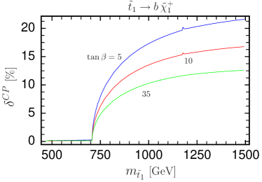
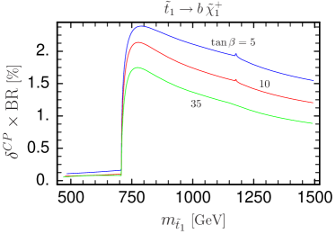
Figure 10.1: $\delta^{CP}$ and $\delta^{CP}\times\mathrm{BR}$ as a function of $m_{\tilde{t}_{1}}$ for various $\tan\beta$, considering all contributions (full one-loop). The parameter $m_{\tilde{t}_{1}}$ is shown for convenience, but the parameter actually varied is $M_{\tilde{Q}}$ from $500$ to $1500$ GeV.

In Fig. 10.2 we show in detail the dominance of the two gluino contributions over the remaining ones by plotting the gluino-to-all ratio. After the threshold at $m_{\tilde{t}_{1}}\sim 708$ GeV ($M_{\tilde{Q}}\sim 719$ GeV), the gluino processes account for $\sim 98\,\%$ of all processes, depending on $\tan\beta$. The kink at $m_{\tilde{t}_{1}}\sim 1175$ GeV (which can be already seen in Fig. 10.1) comes from the threshold of $\tilde{t}_{1}\to t\,\tilde{\chi}^{0}_{3}$, where the graph with $\tilde{\chi}^{0}_{3}-t$ in the stop selfenergy-loop and the two graphs with $H^{\pm}(G^{\pm})-t-\tilde{\chi}^{0}_{3}$ in the vertex correction begin to contribute.

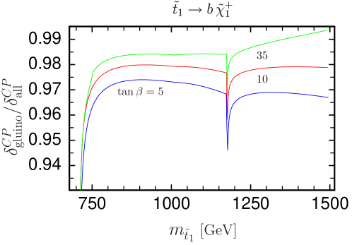
Figure 10.2: Ratio of $\delta^{CP}$ between the two gluino contributions and all contributions (full one-loop) as a function of $m_{\tilde{t}_{1}}$ for various $\tan\beta$. The parameter actually varied is $M_{\tilde{Q}}$ from $719$ to $1500$ GeV.

Fig. 10.3 shows the comparison of the two gluino contributions by plotting their respective $\delta^{CP}$ as a function of $M_{\tilde{Q}}$ from $719$ to $1500$ GeV ($m_{\tilde{t}_{1}}$ is again shown for convenience). Contrary to the expectation that both gluino contributions should dominate due to their strong coupling nature, only the contribution with the gluino in the stop selfenergy-loop accounts for $\delta^{CP}$ in a noteworthy manner. The reason why the vertex correction is so suppressed lies in the $\tilde{b}_{j}-t-\tilde{\chi}^{+}_{1}$ coupling of the Graph 2 in Chapter 9. However, as this coupling is embedded in the one-loop vertex correction in a nontrivial way (see Eq. (9.3)), there exists no simple explanation for this feature.

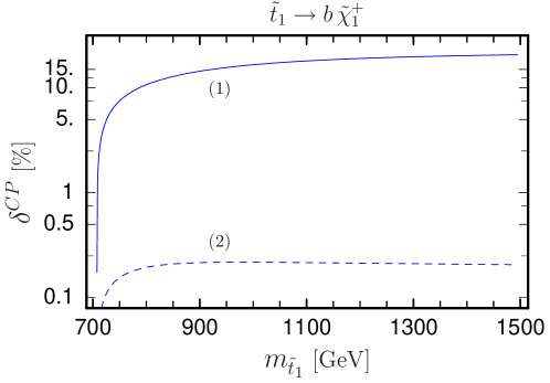
Figure 10.3: Comparison of the two gluino contributions using $\delta^{CP}$ as a function of $m_{\tilde{t}_{1}}$. Label (1) represents the gluino in the selfenergy-loop and (2) the gluino in the vertex-correction. The parameter actually varied is $M_{\tilde{Q}}$ from $719$ to $1500$ GeV.

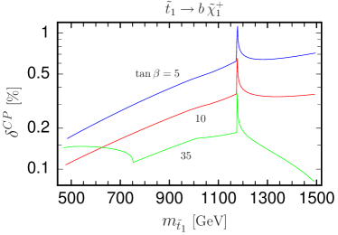
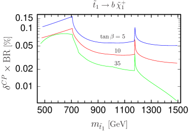
Figure 10.4: $\delta^{CP}$ and $\delta^{CP}\times\mathrm{BR}$ as a function of $m_{\tilde{t}_{1}}$ for various $\tan\beta$, considering all contributions at full one-loop except the two dominant contributions with a gluino. Again, the parameter actually varied is $M_{\tilde{Q}}$ from $500$ to $1500$ GeV.

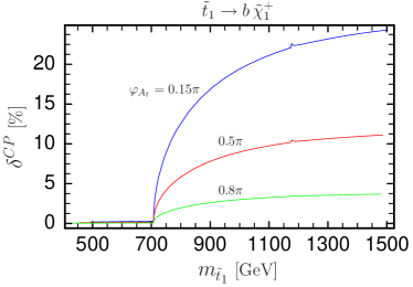
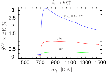
Figure 10.5: $\delta^{CP}$ and $\delta^{CP}\times\mathrm{BR}$ as a function of $m_{\tilde{t}_{1}}$ for various $\varphi_{A_{t}}$, considering all contributions. As always, the parameter actually varied is $M_{\tilde{Q}}$ from $500$ to $1500$ GeV.

In Fig. 10.4 we plot $\delta^{CP}$ as well as $\delta^{CP}\times BR$ as a function of $M_{\tilde{Q}}$ ($m_{\tilde{t}_{1}}$), this time taking all contributions except the two contributions with a gluino. The kink at $m_{\tilde{t}_{1}}\sim 1175$ GeV is the same feature already seen in Fig. 10.1 and 10.2. The kink at $m_{\tilde{t}_{1}}\sim 750$ GeV and $\tan\beta=35$ comes from the closure of the decay channel $\tilde{t}_{1}\to W\,\tilde{b}_{1}$ in the graph with $\tilde{\chi}^{0}_{j}-\tilde{b}_{1}-W$ in the vertex correction. Finally, the kink at $m_{\tilde{t}_{1}}\sim 708$ GeV seen in the $\delta^{CP}\times BR$ plot comes from the branching ratio $BR$ of the decay $\tilde{t}_{1}\to b\,\tilde{\chi}^{+}_{1}$. Since the decay channel into $t\,\tilde{g}$ is now open, it subtracts a lot from $BR$. One again, we can see that the contributions without a gluino can be neglected, if the decay into a gluino and a top is kinematically possible.

In Fig. 10.5 we present $\delta^{CP}$ and $\delta^{CP}\times BR$ as a function of $M_{\tilde{Q}}$ ($m_{\tilde{t}_{1}}$), taking all contributions for various $\varphi_{A_{t}}$. Because the complex phase of $A_{t}$ ($=A_{b,\tau}$) is the only source of CP violation in our chosen scenario, it highly influences $\delta^{CP}$. Taking $\varphi_{A_{t}}=0.15\,\pi$, we obtain the highest value of $\delta^{CP}$ with our parameter set, $\delta^{CP}\sim 24\,\%$ at $m_{\tilde{t}_{1}}=1500$ GeV.

Fig. 10.6 shows the dependence of $\delta^{CP}$ and $\delta^{CP}\times BR$ on $\tan\beta$ for various $M_{\tilde{Q}}$, taking all contributions. The maximal asymmetry lies around $\tan\beta\sim 4\,\%$. The higher the breaking mass parameter $M_{\tilde{Q}}$ (and thus the mass of the decaying particle), the higher the asymmetry $\delta^{CP}$, because more and more decay channels open up and hence more and more processes start to contribute. On the other hand, the more decay channels open up, the less is left for the branching ratio $BR$ of the decay $\tilde{t}_{1}\to b\,\tilde{\chi}^{+}_{1}$.

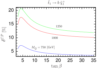
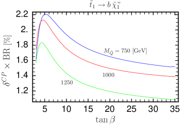
Figure 10.6: $\delta^{CP}$ and $\delta^{CP}\times\mathrm{BR}$ as a function of $\tan\beta$ for various $M_{\tilde{Q}}$, taking all contributions.

In Fig. 10.7 we study the dependence of $\delta^{CP}$ and $\delta^{CP}\times BR$ on $M_{2}$ for various $M_{\tilde{Q}}$, taking all contributions. One can nicely see the closure of the dominating decay channel $\tilde{t}_{1}\to t\,\tilde{g}$, because $M_{2}$ is related to the gluino mass $m_{\tilde{g}}$ via GUT relations. The higher the mass $M_{\tilde{Q}}$ ($m_{\tilde{t}_{1}}$), the later this closure happens. The maximal value of $\delta^{CP}\times BR$ with our parameter set is $\delta^{CP}\times BR\sim 3.5\,\%$ at $M_{2}\sim 370$ GeV and $M_{\tilde{Q}}=1250$ GeV.

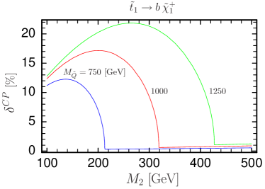
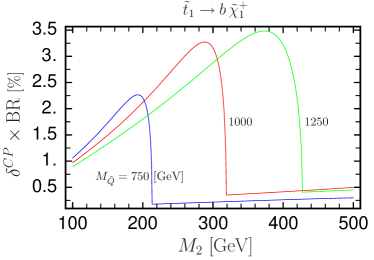
Figure 10.7: $\delta^{CP}$ and $\delta^{CP}\times\mathrm{BR}$ as a function of $M_{2}$ for various $M_{\tilde{Q}}$, taking all contributions.

Fig. 10.8 shows the dependence on the absolute value of the trilinear breaking parameter $|A_{t}|$ for several $\tan\beta$. Here we alter our relation of the breaking mass parameters to $M_{\bar{u}}=1.1\,M_{\tilde{Q}}$, $M_{\bar{d}}=0.8\,M_{\tilde{Q}}$. Otherwise, we would obtain a non-physical result, because of the degeneration of the stop masses (see the main- and off-diagonal elements of the sfermion mass matrix in Eq. (5.1)) which leads to a singularity in the $\tilde{t}_{j}$ propagator of the Graph 1 in Chapter 9. On the other hand, this degeneration would not bother us, if we have not used the approximation done in Eq. (7.8). If we would calculate $\Gamma^{\pm}$ of Eq. (7.4) (and therefore the sum $\Gamma^{+}+\Gamma^{-}$ in $\delta^{CP}$) correctly at full one-loop order using renormalization, this singularity becomes harmless. Due to our relation of the breaking mass parameters, the dependence of the asymmetry on $\tan\beta$ is small.

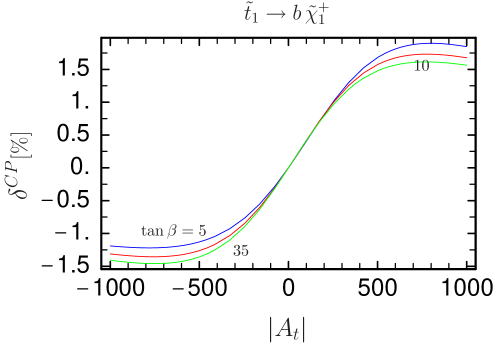
Figure 10.8: $\delta^{CP}$ as a function of $|A_{t}|$ for various $\tan\beta$, taking all contributions and setting $M_{\bar{u}}=1.1\,M_{\tilde{Q}}$, $M_{\bar{d}}=0.8\,M_{\tilde{Q}}$.

In Fig. 10.9 we plot the dependence of $\delta^{CP}$ on $\varphi_{A_{t}}$, taking (a) all contributions and (b) all contributions except the gluino contributions. One can clearly see the periodic dependance on $\varphi_{A_{t}}$. The overall maximum lies at $\varphi_{A_{t}}\sim 0.15\,\pi$ with $\tan\beta=5$.

Figure 10.9: $\delta^{CP}$ as a function of $\varphi_{A_{t}}$ for various $\tan\beta$, taking (a) all contributions and (b) all contributions except the gluino contributions.

Fig. 10.10 shows $\delta^{CP}$ as a function of $|\mu|$ for various $\tan\beta$, considering again all contributions. Because the chargino mass falls below its lower bound, the inner area is ruled out by experiment and thus masked grey. For high $\tan\beta$ the dependence on $|\mu|$ becomes rather symmetric, because the low $\cot\beta$ in the off-diagonal elements in Eq. (5.6) diminishes the dependence on $\mu$. At $|\mu|\sim\pm 300$ GeV we can see the transition of the decaying particle $\tilde{\chi}^{+}_{1}$ between being wino-like (at higher $|\mu|$) and higgsino-like (at lower $|\mu|$), resulting in a different behaviour of the coupling and thus $\delta^{CP}$.

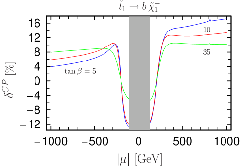
Figure 10.10: $\delta^{CP}$ as a function of $|\mu|$ for various $\tan\beta$, considering all contributions. The inner area is masked out because the chargino mass falls below its lower bound.

Fig. 10.11 with $\delta^{CP}$ as a function of $\varphi_{\mu}$ demonstrates the stringent constraint on the phase of $\mu$, coming from the experimental eEDM-limit. Only a very narrow area is allowed, outside this area we have set $\delta^{CP}$ to zero. As $\tan\beta$ gets bigger, the allowed area reduces even more and therefore we have chosen $\varphi_{\mu}=0$ in our input parameter set in the first place. The negligible dependence of $\delta^{CP}$ on $\varphi_{\mu}$ can be explained with the very narrow parameter range of $\varphi_{\mu}$. Furthermore, the higher $\tan\beta$ gets, the lower the dependence on $\mu$ (due to $\cot\beta$ in Eq. (5.6)) and thus $\varphi_{\mu}$ becomes.

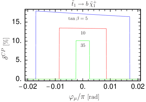
Figure 10.11: $\delta^{CP}$ as a function of $\varphi_{\mu}$ for various $\tan\beta$, considering all contributions. $\delta^{CP}$ is set to zero in the regions not allowed by the experimental eEDM-limit.

For completeness, we also examined the decay of the heavier stop $\tilde{t}_{2}$ into $b\,\tilde{\chi}^{+}_{1}$. Because the two stop particles barely mix in our scenario, their masses are very similar ($m_{\tilde{t}_{1}}=992.10$ GeV and $m_{\tilde{t}_{2}}=1034.73$ GeV). Therefore, the resulting plots are alike, as one can see in Fig. 10.12 in comparison with Fig. 10.1 and also in Fig. 10.13 compared with Fig. 10.4.

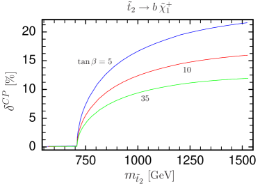
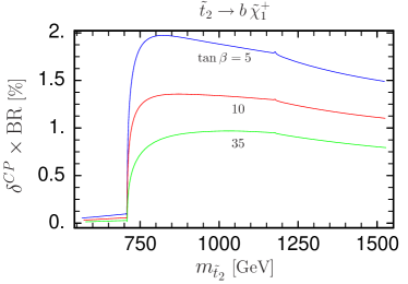
Figure 10.12: $\delta^{CP}$ and $\delta^{CP}\times\mathrm{BR}$ of the decaying particle $\tilde{t}_{2}$ as a function of $m_{\tilde{t}_{2}}$ for various $\tan\beta$, considering all contributions (full one-loop). The parameter $m_{\tilde{t}_{2}}$ is shown for convenience, but the parameter actually varied is $M_{\tilde{Q}}$ from $500$ to $1500$ GeV.

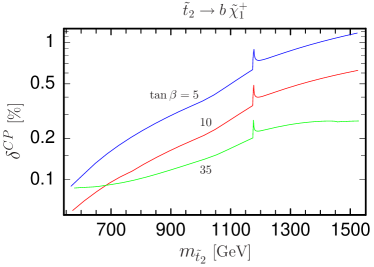
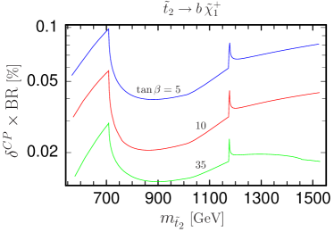
Figure 10.13: $\delta^{CP}$ and $\delta^{CP}\times\mathrm{BR}$ of the decaying particle $\tilde{t}_{2}$ as a function of $m_{\tilde{t}_{2}}$ for various $\tan\beta$, considering all contributions at full one-loop except the two dominant contributions with a gluino. Again, the parameter actually varied is $M_{\tilde{Q}}$ from $500$ to $1500$ GeV.

Finally, we also investigated the influence on the Yukawa couplings $h_{t}$ and $h_{b}$ taken to be running. In our scenario, the difference of the asymmetry $\delta^{CP}$ taken with running Yukawa couplings (tested at two different scales, the mass of the decaying particle and $1000$ GeV) and taken with not running ones is negligible. Only at high values of $M_{\tilde{Q}}=1500$ GeV one obtains a small deviation; not running Yukawa couplings yield a slightly higher asymmetry of $\sim 5\,\%$.

10.2 Conclusions

In this thesis we performed a detailed numerical analysis of the CP violating decay rate asymmetry $\delta^{CP}$ and the quantity $\delta^{CP}\times BR$ of the processes $\tilde{t}_{1}\to b\,\tilde{\chi}^{+}_{1}$ and $\tilde{t}_{2}\to b\,\tilde{\chi}^{+}_{1}$ (and their CP transformed counterparts), analyzing the dependence on the parameters and phases involved.
The asymmetry $\delta^{CP}$ rises up to $\sim 24\,\%$, depending on the point in parameter space. The combined quantity $\delta^{CP}\times\mathrm{BR}$ reaches up to $\sim 3.5\,\%$.
Finally, we want to comment on the feasibility of measuring this asymmetry at the Large Hadron Collider (LHC) at CERN, which will go in operation in summer 2008. As the decaying stop is a strong interacting particle, its production cross section will be large. Therefore, measurement of our decay rate asymmetry $\delta^{CP}$ will be possible at LHC. However, the precise calculation of the measurability is beyond the scope of this thesis, as it involves monte-carlo simulations accounting for all the peculiarities of the detector, among other things.
On the basis of our promising results of the CP violating decay rate asymmetry, we suggest that experimenters should search for evidence of these new CP violating asymmetries in the MSSM, which can be far beyond the small CP violating effects in the SM. These new CP violating sources are not only important in terms of baryogenesis but also very interesting for the further understanding of the subatomic world.

Appendix A Listing of All One-Loop Contributions

Here we specify the complete list of all processes at full one-loop level who can contribute to CP violating asymmetries.

Figure A.1: All vertex contributions who add to the CP violation (Part 1).

Figure A.2: All vertex contributions who add to the CP violation (Part 2).

Figure A.3: All stop-selfenergy contributions who add to the CP violation.

Figure A.4: All chargino-selfenergy contributions who add to the CP violation.

Appendix B Passarino–Veltman Integrals

In this chapter we give the definition of the Passarino–Veltman one-, two-, and three-point functions [57] and list some functions with a special argument set.

B.1 Definitions

We define the Passarino–Veltman one-, two-, and three-point functions in the convention of [58]. For the general denominators we use the notation

$${\mathcal{D}}^{0}=q^{2}-m_{0}^{2}\quad\mbox{and}\quad{\mathcal{D}}^{j}=(q+p_{j})^{2}-m_{j}^{2}\,.$$ (B.1)

Then the loop integrals in $D=4-\epsilon$ dimensions are as follows:

$$A_{0}(m_{0}^{2}) = \frac{1}{i\pi^{2}}\int d^{D}\!q\>\frac{1}{{\mathcal{D}}^{0}}\,,$$ (B.2)

$$B_{0}(p_{1}^{2},m_{0}^{2},m_{1}^{2}) = \frac{1}{i\pi^{2}}\int d^{D}\!q\>\frac{1}{{\mathcal{D}}^{0}{\mathcal{D}}^{1}}\,,$$ (B.3)

$$B_{\mu}(p_{1}^{2},m_{0}^{2},m_{1}^{2}) = \frac{1}{i\pi^{2}}\int d^{D}\!q\>\frac{q_{\mu}}{{\mathcal{D}}^{0}{\mathcal{D}}^{1}}=p_{1\mu}\,B_{1}\,,$$ (B.4)

$$B_{\mu\nu}(p_{1}^{2},m_{0}^{2},m_{1}^{2}) = \frac{1}{i\pi^{2}}\int d^{D}\!q\>\frac{q_{\mu}q_{\nu}}{{\mathcal{D}}^{0}{\mathcal{D}}^{1}}=g_{\mu\nu}\,B_{00}+p_{1\mu}p_{1\nu}\,B_{11}\,,$$ (B.5)

and

$$C_{0} = \frac{1}{i\pi^{2}}\int d^{D}\!q\>\frac{1}{{\mathcal{D}}^{0}{\mathcal{D}}^{1}{\mathcal{D}}^{2}}\,,$$ (B.6)

$$C_{\mu} = \frac{1}{i\pi^{2}}\int d^{D}\!q\>\frac{q_{\mu}}{{\mathcal{D}}^{0}{\mathcal{D}}^{1}{\mathcal{D}}^{2}}=p_{1\mu}C_{1}+p_{2\mu}C_{2}\,,$$ (B.7)

$$C_{\mu\nu} = \frac{1}{i\pi^{2}}\int d^{D}\!q\>\frac{q_{\mu}q_{\nu}}{{\mathcal{D}}^{0}{\mathcal{D}}^{1}{\mathcal{D}}^{2}}$$ (B.8)

$$= g_{\mu\nu}C_{00}+p_{1\mu}p_{1\nu}C_{11}+(p_{1\mu}p_{2\nu}+p_{2\mu}p_{1\nu})C_{12}+p_{2\mu}p_{2\nu}C_{22}\,,$$

where the $C$’s have $(p_{1}^{2},(p_{1}-p_{2})^{2},p_{2}^{2},m_{0}^{2},m_{1}^{2},m_{2}^{2})$ as their arguments. For further details about the coefficient functions, some reductions and relations, some analytical expressions and some special argument sets see [46].

B.2 Special Argument Set

Here we list the Passarino–Veltman integrals with a special argument set needed in Appendix F. All masses of the external particles are set to zero ($p_{1}^{2}=(p_{1}-p_{2})^{2}=p_{2}^{2}=0$) and two of the internal particles are the same.
For the scalar B-function we obtain (see [46])

$$B_{0}(0,M_{1}^{2},M_{1}^{2})=\Delta+\log\left(\frac{Q^{2}}{M_{1}^{2}}\right)$$ (B.9)

with the real UV-divergence parameter $\Delta=\frac{2}{\epsilon}-\gamma+\log(4\pi)$, the Euler-Mascheroni Constant $\gamma\sim 0.577216$ and the scale parameter $Q$.
Using Feynman parametrization we derive for the scalar C-function

$$C_{0}(f)=\frac{1-x+\log(x)}{M_{0}^{2}(1-x)^{2}}$$ (B.10)

with $x=M_{1}^{2}/M_{0}^{2}$ and $f=(0,0,0,M_{0}^{2},M_{1}^{2},M_{1}^{2})$.
The coefficient functions take the form

$$C_{1}(f) = -\frac{3-4x+x^{2}+2\log(x)}{4M_{0}^{2}(1-x)^{3}}$$ (B.11)

$$C_{00}(f) = \frac{1}{4}\bigg{(}\Delta+\log\left(\frac{Q^{2}}{M_{1}^{2}}\right)+1+\frac{1-x^{2}+2\log(x)}{2(1-x)^{2}}\bigg{)}$$ (B.12)

$$C_{11}(f)+C_{12}(f) = \frac{11-18x+9x^{2}-2x^{3}+6\log(x)}{12M_{0}^{2}(1-x)^{4}}\,.$$ (B.13)

In our special case, the relations $C_{1}\sim C_{2}$ and $C_{11}+C_{12}\sim C_{22}+C_{12}$ hold.

Appendix C Calculation of a Generic Structure

We show the calculation of a generic structure taking the generic structure I in Section 9.2 as an example. First, we only take the matrix elements of the three vertices alone:

$${\cal M}_{0} = i\,\bar{u}(k_{1})(g_{0}^{R}P_{R}+g_{0}^{L}P_{L})v(-k_{2})$$ (C.1)

$${\cal M}_{1} = i\,\bar{u}(q+p)(g_{1}^{R}P_{R}+g_{1}^{L}P_{L})v(-q)$$ (C.2)

$${\cal M}_{2} = i\,\bar{u}(q)(g_{2}^{R}P_{R}+g_{2}^{L}P_{L})v(-(q+p)).$$ (C.3)

Then we can write down the matrix element of the selfenergy loop from ${\cal M}_{1}$ and ${\cal M}_{2}$ using Feynman rules. Because of the closed fermion loop we introduce an additional overall factor $(-1)$ (for a detailed derivation see [46]). We obtain

$${\cal{M}}_{\mathrm{self}}=-\int\frac{\mathrm{d}^{4}q}{(2\pi)^{4}}\frac{1}{D_{0}D_{1}}X$$ (C.4)

where we used the abbreviations

$$D_{0} = q^{2}-M_{1}^{2}$$ (C.5)

$$D_{1} = (q+p)^{2}-M_{2}^{2}$$ (C.6)

$$X = \mathrm{Tr}\bigl{[}(g_{1}^{R}P_{R}+g_{1}^{L}P_{L})(\not{q}+M_{1})(g_{2}^{R}P_{R}+g_{2}^{L}P_{L})(\not{q}+\not{p}+M_{2})\bigr{]}.$$ (C.7)

We can modify $X$ to

$$X = \mathrm{Tr}\bigl{[}\not{q}(\not{q}+\not{p})(g_{1}^{R}g_{2}^{L}P_{R}+g_{1}^{L}g_{2}^{R}P_{L})+\not{q}M_{2}(g_{1}^{L}g_{2}^{R}P_{R}+g_{1}^{R}g_{2}^{L}P_{L})$$ (C.8)

$$+(\not{q}+\not{p})M_{1}(g_{1}^{L}g_{2}^{L}P_{R}+g_{1}^{R}g_{2}^{R}P_{L})+M_{1}M_{2}(g_{1}^{R}g_{2}^{R}P_{R}+g_{1}^{L}g_{2}^{L}P_{L})\bigr{]}$$

$$= 2(q^{2}+(q.p))(g_{1}^{R}g_{2}^{L}+g_{1}^{L}g_{2}^{R})+2M_{1}M_{2}(g_{1}^{R}g_{2}^{R}+g_{1}^{L}g_{2}^{L})$$

using the relations $P_{R,L}^{2}=P_{R,L}$, $P_{R,L}P_{L,R}=0$ and $\mathrm{Tr}(P_{R,L})=2$, $\mathrm{Tr}(\not{a}\not{b}P_{R,L})=2(a.b)$, $\mathrm{Tr}(\not{a}P_{R,L})=0$.
Now we switch from $4$ to $D=4-\epsilon$ dimensions using the SUSY invariant Dimensional Reduction regularization scheme $\overline{\mathrm{DR}}$ resulting in $\mathrm{d}^{4}q/(2\pi)^{4}\to\mathrm{d}^{D}q/(2\pi)^{D}$. Substituting this and Eq. (C.8) into Eq. (C.7) results in

$${\cal{M}}_{\mathrm{self}}=-\int\frac{\mathrm{d}^{D}q}{(2\pi)^{D}}\frac{1}{D_{0}D_{1}}\Bigl{[}2(q^{2}+(q.p))(g_{1}^{R}g_{2}^{L}+g_{1}^{L}g_{2}^{R})+2M_{1}M_{2}(g_{1}^{R}g_{2}^{R}+g_{1}^{L}g_{2}^{L})\Bigr{]}.$$ (C.9)

For the calculation of the loop integrals we use the formalism of Passarino–Veltman Integrals introduced in Appendix B. Using Eq. (B.3), (B.4) and Eq. (B.5) reduced with the metric tensor $g^{\mu\nu}$ we get

$$\int\frac{\mathrm{d}^{D}q}{(2\pi)^{D}}\frac{1}{D_{0}D_{1}} = \frac{i}{(4\pi)^{2}}B_{0}$$ (C.10)

$$\int\frac{\mathrm{d}^{D}q}{(2\pi)^{D}}\frac{(q.p)}{D_{0}D_{1}} = \frac{i}{(4\pi)^{2}}p^{2}B_{1}$$ (C.11)

$$\int\frac{\mathrm{d}^{D}q}{(2\pi)^{D}}\frac{q^{2}}{D_{0}D_{1}} = \frac{i}{(4\pi)^{2}}(4B_{00}+p^{2}B_{11})$$ (C.12)

where the B-functions have $(p^{2},M_{1}^{2},M_{2}^{2})$ as their arguments. The matrix element then becomes

$${\cal{M}}_{\mathrm{self}} = -\frac{i}{(4\pi)^{2}}\bigg{[}2\Big{(}4B_{00}+m_{0}^{2}(B_{1}+B_{11})\Big{)}(g_{1}^{R}g_{2}^{L}+g_{1}^{L}g_{2}^{R})$$ (C.13)

$$+2M_{1}M_{2}\Big{(}g_{1}^{R}g_{2}^{R}+g_{1}^{L}g_{2}^{L}\Big{)}B_{0}\bigg{]}$$

$$= -\frac{i}{(4\pi)^{2}}\bigg{[}\Big{(}A_{0}(M_{1}^{2})+A_{0}(M_{2}^{2})+(M_{1}^{2}+M_{2}^{2}-m_{0}^{2})B_{0}\Big{)}(g_{1}^{R}g_{2}^{L}+g_{1}^{L}g_{2}^{R})$$

$$+2M_{1}M_{2}\Big{(}g_{1}^{R}g_{2}^{R}+g_{1}^{L}g_{2}^{L}\Big{)}B_{0}\bigg{]}$$

where we used the on-shell relation $p^{2}=m_{0}^{2}$ and reduced the term with $B_{1}$, $B_{00}$ and $B_{11}$ down to $A_{0}$ and $B_{0}$ using equations found in [46]. The matrix element of the final graph is then derived from Eq. (C.1) and (C.13)

$$\mathcal{M} = {\cal{M}}_{\mathrm{self}}\,\frac{i}{p^{2}-M_{0}^{2}}\,\mathcal{M}_{0}$$ (C.14)

$$= \frac{i}{(4\pi)^{2}}\bar{u}(k_{1})(\Lambda_{R}P_{R}+\Lambda_{L}P_{L})v(-k_{2})$$

with the form factors

$$\Lambda_{R} = \frac{1}{m_{0}^{2}-M_{0}^{2}}g_{0}^{R}\bigg{[}\Big{(}A_{0}(M_{1}^{2})+A_{0}(M_{2}^{2})+(M_{1}^{2}+M_{2}^{2}-m_{0}^{2})B_{0}\Big{)}(g_{1}^{R}g_{2}^{L}+g_{1}^{L}g_{2}^{R})$$ (C.15)

$$+2M_{1}M_{2}\Big{(}g_{1}^{R}g_{2}^{R}+g_{1}^{L}g_{2}^{L}\Big{)}B_{0}\bigg{]}$$

$$\Lambda_{L} = \Lambda_{R}\,(R\leftrightarrow L)$$ (C.16)

just like in Eq. (9.2).

Appendix D Calculation of a Coupling

As an example for the calculation of couplings we derive the tree level interaction of a chargino with a sfermion-fermion pair $\tilde{\chi}^{+}f\tilde{f}^{\prime}$ as specified in Chapter 6.
Since charginos as well as sfermions are mass eigenstates that are formed out of a mixing of interaction eigenstates, one has to consider the Lagrangian of interaction eigenstates first. The relevant terms are derived from the superpotential and the SUSY gauge coupling terms (for a detailed derivation see [45]). We obtain

$$\mathcal{L}_{\tilde{\chi}^{+}f\tilde{f}^{\prime}} = \mathcal{L}^{\mathrm{int}}_{\mathrm{Yuk}}+\mathcal{L}^{\mathrm{int}}_{\mathrm{weak}}\,,$$ (D.1)

$$\mathcal{L}^{\mathrm{int}}_{\mathrm{Yuk}} = h_{t}(\tilde{t}^{*}_{R}b_{L}+\tilde{b}_{L}t^{\dagger}_{R})\psi^{1}_{H_{2}}+h_{b}(\tilde{b}^{*}_{R}t_{L}+\tilde{t}_{L}b^{\dagger}_{R})\psi^{2}_{H_{1}}$$ (D.2)

$$+h_{\tau}(\tilde{\tau}^{*}_{R}\nu_{\tau}+\tilde{\nu}_{\tau}\tau^{\dagger}_{R})\psi^{2}_{H_{1}}+h.c.\,,$$

$$\mathcal{L}^{\mathrm{int}}_{\mathrm{weak}} = ig\Bigl{[}(\tilde{t}^{*}_{L}b_{L}+\tilde{\nu}^{*}_{\tau}\tau_{L})\lambda^{+}+(\tilde{b}^{*}_{L}t_{L}+\tilde{\tau}^{*}_{L}\nu_{\tau})\lambda^{-}+h.c.\Bigr{]}\,.$$ (D.3)

Then we transform the Lagrangians to mass eigenstates using the relations (5.10, 5.15) resulting in

$$\mathcal{L}^{\mathrm{int}}_{\mathrm{Yuk}} = h_{t}(R^{\tilde{t}}_{i2}\tilde{t}^{*}_{i}b_{L}+R^{\tilde{b}*}_{i1}\tilde{b}_{i}t^{\dagger}_{R})V^{*}_{k2}\chi^{+}_{k}+h_{b}(R^{\tilde{b}}_{i2}\tilde{b}^{*}_{i}t_{L}+R^{\tilde{t}*}_{i1}\tilde{t}_{i}b^{\dagger}_{R})U^{*}_{k2}\chi^{-}_{k}$$ (D.4)

$$+h_{\tau}(R^{\tilde{\tau}}_{i2}\tilde{\tau}^{*}_{i}\nu_{\tau}+\tilde{\nu}_{\tau}\tau^{\dagger}_{R})U^{*}_{k2}\chi^{-}_{k}+h.c.\,,$$

$$\mathcal{L}^{\mathrm{int}}_{\mathrm{weak}} = -g\bigl{[}(R^{\tilde{t}}_{i1}\tilde{t}^{*}_{i}b_{L}+\tilde{\nu}^{*}_{\tau}\tau_{L})V^{*}_{k1}\chi^{+}_{k}$$ (D.5)

$$+(R^{\tilde{b}}_{i1}\tilde{b}^{*}_{i}t_{L}+R^{\tilde{\tau}}_{i1}\tilde{\tau}^{*}_{i}\nu_{\tau})U^{*}_{k1}\chi^{-}_{k}+h.c.\bigr{]}\,.$$

Summing up the results we gain

$$\mathcal{L}_{\tilde{\chi}^{+}f\tilde{f}^{\prime}} = (h_{t}R^{\tilde{t}}_{i2}V^{*}_{k2}-gR^{\tilde{t}}_{i1}V^{*}_{k1})\tilde{t}^{*}_{i}b_{L}\chi^{+}_{k}+h_{t}R^{\tilde{b}*}_{i1}V^{*}_{k2}\tilde{b}_{i}\tilde{t}^{\dagger}_{R}\chi^{+}_{k}-gV^{*}_{k1}\tilde{\nu}^{*}_{\tau}\tau_{L}\chi^{+}_{k}$$ (D.6)

$$+(h_{b}R^{\tilde{b}}_{i2}U^{*}_{k2}-gR^{\tilde{b}}_{i1}U^{*}_{k1})\tilde{b}^{*}_{i}t_{L}\chi^{-}_{k}+h_{b}R^{\tilde{t}*}_{i1}U^{*}_{k2}\tilde{t}_{i}\tilde{b}^{\dagger}_{R}\chi^{-}_{k}$$

$$+(h_{\tau}R^{\tilde{\tau}}_{i2}U^{*}_{k2}-gR^{\tilde{\tau}}_{i1}U^{*}_{k1})\tilde{\tau}^{*}_{i}\nu_{\tau}\chi^{-}_{k}+h_{\tau}U^{*}_{k2}\tilde{\nu}_{\tau}\tau^{\dagger}_{R}\chi^{-}_{k}+h.c.\,.$$

Finally we transform the Weyl spinors to Dirac spinors using the relations (E.14, E.15) and separate the Lagrangian into a chargino-squark-quark and a chargino-slepton-lepton part $\mathcal{L}_{\tilde{\chi}^{+}f\tilde{f}^{\prime}}=\mathcal{L}_{\tilde{\chi}^{+}q\tilde{q}^{\prime}}+\mathcal{L}_{\tilde{\chi}^{+}l\tilde{l}^{\prime}}$. We get

$${\cal L}_{\tilde{\chi}^{+}q\tilde{q}^{\prime}} = \bar{t}(A^{R}_{ki}P_{R}+A^{L}_{ki}P_{L})\tilde{\chi}^{+}_{k}\tilde{b}_{i}+\bar{b}(B^{R}_{ki}P_{R}+B^{L}_{ki}P_{L})\tilde{\chi}^{-}_{k}\tilde{t}_{i}$$ (D.7)

$$+\overline{\tilde{\chi}^{+}_{k}}(A^{L*}_{ki}P_{R}+A^{R*}_{ki}P_{L})t\tilde{b}^{*}_{i}+\overline{\tilde{\chi}^{-}_{k}}(B^{L*}_{ki}P_{R}+B^{R*}_{ki}P_{L})b\tilde{t}^{*}_{i}\,,$$

$${\cal L}_{\tilde{\chi}^{+}l\tilde{l}^{\prime}} = \bar{\nu}_{\tau}(A^{\prime R}_{ki}P_{R}+A^{\prime L}_{ki}P_{L})\tilde{\chi}^{+}_{k}\tilde{\tau}_{i}+\bar{\tau}(B^{\prime R}_{k}P_{R}+B^{\prime L}_{k}P_{L})\tilde{\chi}^{-}_{k}\tilde{\nu}_{\tau}$$ (D.8)

$$+\overline{\tilde{\chi}^{+}_{k}}(A^{\prime L*}_{ki}P_{R}+A^{\prime R*}_{ki}P_{L})\nu_{\tau}\tilde{\tau}^{*}_{i}+\overline{\tilde{\chi}^{-}_{k}}(B^{\prime L*}_{k}P_{R}+B^{\prime R*}_{k}P_{L})\tau\tilde{\nu}^{*}_{\tau}\,,$$

with the projection operators $P_{R,L}=(1\pm\gamma^{5})/2$.
The abbreviated coupling matrices, which can be further transformed using $m_{W}=g\nu/2$, $m_{t}=(h_{t}\nu\sin\beta)/\sqrt{2}$ and $m_{b}=(h_{b}\nu\cos\beta)/\sqrt{2}$, are

$$A^{R}_{ki} = h_{b}R^{\tilde{b}*}_{i2}U_{k2}-gR^{\tilde{b}*}_{i1}U_{k1}$$

$$= \frac{g}{\sqrt{2}}\left(\frac{m_{b}}{m_{W}\cos\beta}U_{k2}R^{\tilde{b}*}_{i2}-\sqrt{2}U_{k1}R^{\tilde{b}*}_{i1}\right)\,,$$

$$A^{L}_{ki} = h_{t}R^{\tilde{b}*}_{i1}V^{*}_{k2}=\frac{gm_{t}}{\sqrt{2}m_{W}\sin\beta}V^{*}_{k2}R^{\tilde{b}*}_{i1}\,,$$

$$B^{R}_{ki} = h_{t}R^{\tilde{t}*}_{i2}V_{k2}-gR^{\tilde{t}*}_{i1}V_{k1}$$

$$= \frac{g}{\sqrt{2}}\left(\frac{m_{t}}{m_{W}\sin\beta}V_{k2}R^{\tilde{t}*}_{i2}-\sqrt{2}V_{k1}R^{\tilde{t}*}_{i1}\right)\,,$$

$$B^{L}_{ki} = h_{b}R^{\tilde{t}*}_{i1}U^{*}_{k2}=\frac{gm_{b}}{\sqrt{2}m_{W}\cos\beta}U^{*}_{k2}R^{\tilde{t}*}_{i1}\,,$$ (D.9)

$$A^{\prime R}_{ki} = h_{\tau}R^{\tilde{\tau}*}_{i2}U_{k2}-gR^{\tilde{\tau}*}_{i1}U_{k1}$$

$$= \frac{g}{\sqrt{2}}\left(\frac{m_{\tau}}{m_{W}\cos\beta}U_{k2}R^{\tilde{\tau}*}_{i2}-\sqrt{2}U_{k1}R^{\tilde{\tau}*}_{i1}\right)\,,$$

$${A^{\prime}}^{L}_{ki} = 0\,,$$

$$B^{\prime R}_{k} = -gV_{k1}\,,$$

$$B^{\prime L}_{k} = h_{\tau}U^{*}_{k2}=\frac{gm_{\tau}}{\sqrt{2}m_{W}\cos\beta}U^{*}_{k2}\,,$$ (D.10)

just like in (6.3) and (6.4). These coupling matrices as well as the Lagrangians have the same convention as in [20].

Appendix E Transformation of Weyl to Dirac Spinors

We define a four component Dirac spinor as follows

$$\Psi={\chi\choose\bar{\psi}},$$ (E.1)

where the two quantities $\chi$ and $\psi$ are two component Weyl spinors, standing for particle and anti-particle, respectively.
We choose the chiral representation so the gamma matrices $\gamma^{0}$ and $\gamma^{5}$ and the projection operators $P_{R,L}$ as well as the adjoint Dirac spinor $\bar{\Psi}$ are:

$$\gamma^{0}=\left(\begin{array}[]{cc}0&1\\ 1&0\end{array}\right)\qquad\gamma^{5}=\left(\begin{array}[]{cc}-1&0\\ 0&1\end{array}\right),$$ (E.2)

$$P_{R} = \frac{1}{2}(1+\gamma^{5})=\left(\begin{array}[]{cc}0&0\\ 0&1\end{array}\right),$$ (E.5)

$$P_{L} = \frac{1}{2}(1-\gamma^{5})=\left(\begin{array}[]{cc}1&0\\ 0&0\end{array}\right),$$ (E.8)

$$\bar{\Psi}=\Psi^{\dagger}\gamma^{0}=(\psi\;\bar{\chi})\,.$$ (E.9)

With these relations one can now carry out all sorts of transformations including products of Weyl spinors

$$\psi_{1}\chi_{2}=\bar{\Psi}_{1}P_{L}\Psi_{2}\qquad\bar{\chi}_{1}\bar{\psi}_{2}=\bar{\Psi}_{1}P_{R}\Psi_{2}\,.$$ (E.10)

We define the fermions of the SM, the charginos as well as the neutralinos

$$t={t_{L}\choose t_{R}}\quad\bar{t}=(t^{\dagger}_{R}\;t^{\dagger}_{L}) b={b_{L}\choose b_{R}}\quad\bar{b}=(b^{\dagger}_{R}\;b^{\dagger}_{L})\,,$$

$$\nu_{\tau}={\nu_{\tau}\choose 0}\quad\bar{\nu}_{\tau}=(0\;\nu_{\tau}^{\dagger}) \tau={\tau_{L}\choose\tau_{R}}\quad\bar{\tau}=(\tau^{\dagger}_{R}\;\tau^{\dagger}_{L})\,,$$ (E.11)

$$\tilde{\chi}^{+}_{k}={\chi^{+}_{k}\choose\bar{\chi}^{-}_{k}}\quad\overline{\tilde{\chi}^{+}_{k}}=(\chi^{-}_{k}\;\bar{\chi}^{+}_{k}) \tilde{\chi}^{-}_{k}={\chi^{-}_{k}\choose\bar{\chi}^{+}_{k}}\quad\overline{\tilde{\chi}^{-}_{k}}=(\chi^{+}_{k}\;\bar{\chi}^{-}_{k})\,,$$ (E.12)

$$\tilde{\chi}^{0}_{k}={\chi^{0}_{k}\choose\bar{\chi}^{0}_{k}} \overline{\tilde{\chi}^{0}_{k}}=(\chi^{0}_{k}\;\bar{\chi}^{0}_{k})\,.$$ (E.13)

Therefore we obtain for example the following transformations using Eq. (E.10)

$$t_{L}\chi^{-}_{k}=\overline{\tilde{\chi}^{+}_{k}}P_{L}t b_{L}\chi^{+}_{k}=\overline{\tilde{\chi}^{-}_{k}}P_{L}b\,,$$

$$t^{\dagger}_{R}\chi^{+}_{k}=\bar{t}P_{L}\tilde{\chi}^{+}_{k} b^{\dagger}_{R}\chi^{-}_{k}=\bar{b}P_{L}\tilde{\chi}^{-}_{k}\,,$$

$$t_{L}\chi^{0}_{k}=\overline{\tilde{\chi}^{0}_{k}}P_{L}t b_{L}\chi^{0}_{k}=\overline{\tilde{\chi}^{0}_{k}}P_{L}b\,,$$

$$t^{\dagger}_{R}\chi^{0}_{k}=\bar{t}P_{L}\tilde{\chi}^{0}_{k} b^{\dagger}_{R}\chi^{0}_{k}=\bar{b}P_{L}\tilde{\chi}^{0}_{k}\,,$$ (E.14)

$$\tau_{L}\chi^{+}_{k}=\overline{\tilde{\chi}^{-}_{k}}P_{L}\tau \tau^{\dagger}_{R}\chi^{-}_{k}=\bar{\tau}P_{L}\tilde{\chi}^{-}_{k} \nu_{\tau}\chi^{-}_{k}=\overline{\tilde{\chi}^{+}_{k}}P_{L}\nu_{\tau}\,,$$

$$\tau_{L}\chi^{0}_{k}=\overline{\tilde{\chi}^{0}_{k}}P_{L}\tau \tau^{\dagger}_{R}\chi^{0}_{k}=\bar{\tau}P_{L}\tilde{\chi}^{0}_{k} \nu_{\tau}\chi^{0}_{k}=\overline{\tilde{\chi}^{0}_{k}}P_{L}\nu_{\tau}\,.$$ (E.15)

Appendix F The Electric Dipole Moment (EDM)

The additional CP-violating phases in the MSSM are new sources of CP violation beyond the SM. From the point of view of baryogenesis, one hopes that these phases are large [6, 7, 8, 9]. But the experimental limits on electron and neutron electric dipole moments (EDMs), $|d_{e}|\leq 1.6\times 10^{-27}\,[e\times\mathrm{cm}]$ [59] and $|d_{n}|\leq 2.9\times 10^{-26}\,[e\times\mathrm{cm}]$ [60], place constraints on the CP violating phases of the MSSM. Especially the complex phase of $\mu$ is severely constrained with about $\phi_{\mu}<\mathcal{O}(10^{-2})$ [61, 62, 63, 64] for a typical SUSY mass scale of the order of a few hundred GeV. A larger $\phi_{\mu}$ imposes fine-tuned relationships between this phase and other SUSY parameters [65, 66, 67].
In this chapter we calculate the EDM of an electron. We start by giving the relevant generic structures and then derive the EDM of a fermion. We apply this result to compute the EDM of the electron and point out some numerical issues. Finally we use this calculation as an automatic checkup-routine in our calculation of CP violating asymmetries so as to make sure our chosen complex parameter set of the MSSM is not already ruled out by experiment.

F.1 Generic Structures

Here we list the two generic structures which are needed for the calculation of the EDM of a fermion. Note that we rotated these two generic vertex corrections to fit the generic structures found in [46]. The convention for the momenta and the masses from Chapter 9 still applies but is of course rotated as well.
The generic matrix element is

$$\mathcal{M}=\frac{i}{(4\pi)^{2}}\epsilon_{\mu}(p)\bar{u}(k_{1})(\gamma^{\mu}A_{i}+k^{\mu}B_{i}+p^{\mu}C_{i})P_{i}v(-k_{2})$$ (F.1)

with $i\in\{R,L\}$. The form factors $A_{L}$, $B_{L}$ and $C_{L}$ can be again easily obtained by exchanging right- and left-handed couplings $(g^{R}\leftrightarrow g^{L})$.
The first generic structure is a scalar-fermion-fermion vertex correction.

0 : $i\gamma^{\mu}(g_{0}^{R}P_{R}+g_{0}^{L}P_{L})$ 1 : $i(g_{1}^{R}P_{R}+g_{1}^{L}P_{L})$ 2 : $i(g_{2}^{R}P_{R}+g_{2}^{L}P_{L})$

The appropriate form factors are

$$A^{I}_{R}(f) = -\bigg{(}g_{0}^{L}g_{1}^{L}g_{2}^{R}\Big{(}2C_{00}-B_{0}(m_{0}^{2},M_{1}^{2},M_{2}^{2})\Big{)}+(g_{0}^{R}h_{1}^{RL}h_{2}^{LR}-g_{0}^{L}g_{1}^{L}g_{2}^{R}M_{0}^{2})C_{0}$$ (F.2)

$$+(g_{0}^{R}g_{1}^{R}h_{2}^{LR}-g_{0}^{L}g_{2}^{R}h_{1}^{LR})m_{1}C_{1}-(g_{0}^{L}g_{1}^{L}h_{2}^{RL}-g_{0}^{R}g_{2}^{L}h_{1}^{RL})m_{2}C_{2}\bigg{)}\,,$$

$$B^{I}_{R}(f) = -\Big{(}g_{0}^{L}g_{2}^{R}h_{1}^{LR}C_{1}+g_{0}^{R}g_{1}^{R}h_{2}^{LR}C_{2}$$ (F.3)

$$+g_{0}^{L}g_{1}^{L}g_{2}^{R}m_{1}(C_{11}+C_{12})+g_{0}^{R}g_{1}^{R}g_{2}^{L}m_{2}(C_{22}+C_{12})\Big{)}\,,$$

$$C^{I}_{R}(f) = -\Big{(}g_{0}^{L}g_{2}^{R}h_{1}^{LR}C_{1}-g_{0}^{R}g_{1}^{R}h_{2}^{LR}C_{2}$$ (F.4)

$$+g_{0}^{L}g_{1}^{L}g_{2}^{R}m_{1}(C_{11}-C_{12})-g_{0}^{R}g_{1}^{R}g_{2}^{L}m_{2}(C_{22}-C_{12})\Big{)}$$

with the auxiliary functions

$$h_{i}^{jk}=g_{i}^{j}m_{i}+g_{i}^{k}M_{i}\qquad i\in\{1,2\}\,;\,j,k\in\{L,R\}$$ (F.5)

where we do not sum over the index $i$. The argument set is

$$f=(m_{0},m_{1},m_{2},M_{0},M_{1},M_{2},g_{0}^{R},g_{0}^{L},g_{1}^{R},g_{1}^{L},g_{2}^{R},g_{2}^{L})\,.$$ (F.6)

The second generic structure is a fermion-scalar-scalar vertex correction.

0 : $ig_{0}(2q+k_{1}+k_{2})^{\mu}$ 1 : $i(g_{1}^{R}P_{R}+g_{1}^{L}P_{L})$ 2 : $i(g_{2}^{R}P_{R}+g_{2}^{L}P_{L})$

The appropriate form factors are

$$A^{II}_{R}(f) = 2C_{00}g_{0}g_{1}^{L}g_{2}^{R}\,,$$ (F.7)

$$B^{II}_{R}(f) = g_{0}\Big{(}m_{1}g_{1}^{L}g_{2}^{R}(C_{1}+C_{11}+C_{12})+m_{2}g_{1}^{R}g_{2}^{L}(C_{2}+C_{22}+C_{12})$$ (F.8)

$$-M_{0}g_{1}^{R}g_{2}^{R}(C_{0}+C_{1}+C_{2})\Big{)}\,,$$

$$C^{II}_{R}(f) = g_{0}\Big{(}m_{1}g_{1}^{L}g_{2}^{R}(C_{11}-C_{12})-m_{2}g_{1}^{R}g_{2}^{L}(C_{22}-C_{12})$$ (F.9)

$$-M_{0}g_{1}^{R}g_{2}^{R}(C_{1}-C_{2})\Big{)}$$

with the argument set $f=(m_{0},m_{1},m_{2},M_{0},M_{1},M_{2},g_{0},g_{1}^{R},g_{1}^{L},g_{2}^{R},g_{2}^{L})$.

F.2 Electric Dipole Moment of a Fermion

Now we are ready for the calculation of the EDM of a fermion. We start with the matrix element in Eq. (F.1) and apply the Gordon decomposition in order to obtain the $\sigma^{\mu\nu}$-terms which describe the spin exchange of the two fermions. Then we use these terms to derive the EDM using the relations found in [68].
The Gordon decomposition takes the general form

$$\bar{u}(p^{\prime})\gamma^{\mu}P_{i}u(p)=\frac{1}{2m}\bar{u}(p^{\prime})(p^{\prime}+p)^{\mu}P_{i}u(p)+\bar{u}(p^{\prime})i\frac{\sigma^{\mu\nu}}{2m}(p^{\prime}-p)_{\nu}P_{i}u(p)$$ (F.10)

with $i\in\{R,L\}$. Using this relation one can transform the first two terms in Eq. (F.1) and we obtain

$$\mathcal{M} = \frac{i}{(4\pi)^{2}}\epsilon_{\mu}(p)\bigg{(}A_{i}\Big{(}\frac{1}{2m_{f}}\bar{u}(k_{1})k^{\mu}P_{i}u(k_{2})+\bar{u}(k_{1})i\frac{\sigma^{\mu\nu}}{2m_{f}}p_{\nu}P_{i}u(k_{2})\Big{)}$$ (F.11)

$$+B_{i}\Big{(}2m_{f}\bar{u}(k_{1})\gamma^{\mu}P_{i}u(k_{2})-i\bar{u}(k_{1})\sigma^{\mu\nu}p_{\nu}P_{i}u(k_{2})\Big{)}\bigg{)}\,.$$

Taking only the terms with $\sigma^{\mu\nu}$ and rearranging a bit yields for the amplitude $T$ ($\mathcal{M}^{\sigma^{\mu\nu}}=iT$) (see [68])

$$T=ie\epsilon_{\mu}(p)\frac{p_{\nu}}{2m_{f}}\bar{u}(k_{1})\sigma^{\mu\nu}(a^{R}P_{R}+a^{L}P_{L})u(k_{2})$$ (F.12)

with the coefficients

$$a^{R} = \frac{1}{e(4\pi)^{2}}(A_{R}-2m_{f}B_{R})$$ (F.13)

$$a^{L} = \frac{1}{e(4\pi)^{2}}(A_{L}-2m_{f}B_{L})\,.$$ (F.14)

The EDM of a fermion is then calculated by the simple formula

$$d_{f}=-\frac{e}{4m_{f}}\mathrm{Im}(a^{R}-a^{L})\,.$$ (F.15)

F.3 Electric Dipole Moment of the Electron (eEDM)

There are two processes who contribute to the EDM of the electron, one with a sneutrino-chargino and one with a selectron-neutralino in the loop (see Fig. F.1).

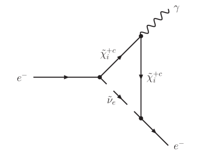
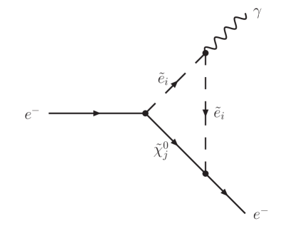
Figure F.1: The two processes who contribute to the eEDM. On the left a sneutrino-chargino and on the right a selectron-neutralino in the loop.

The form factors for the sneutrino-chargino contribution have the following arguments

$$A^{1}_{R,L} = \sum_{i=1}^{2}A^{I}_{R,L}(0,m_{e},m_{e},m_{\tilde{\nu}_{e}},m_{\tilde{\chi}^{+}_{i}},m_{\tilde{\chi}^{+}_{i}},e,e,B^{\prime R}_{i},B^{\prime L}_{i},B^{\prime L*}_{i},B^{\prime R*}_{i})$$ (F.16)

and analogously for $B^{1}_{R,L}$.
The form factors for the selectron-neutralino contribution have the following arguments

$$A^{2}_{R,L} = \sum_{i=1}^{2}\sum_{j=1}^{4}A^{II}_{R,L}(0,m_{e},m_{e},m_{\tilde{\chi}^{0}_{j}},m_{\tilde{e}_{i}},m_{\tilde{e}_{i}},e,D^{\prime R}_{ji},D^{\prime L}_{ji},D^{\prime L*}_{ji},D^{\prime R*}_{ji})$$ (F.17)

and analogously for $B^{2}_{R,L}$.
Because of the huge masses of the particles in the loop compared to the mass of the external electron, one has to carefully avoid numerical instabilities. Especially the Passarino–Veltman integrals, where we set the electron mass to zero, need special treatment. As now all three external particles are massless, we have to use the special Passarino–Veltman integrals derived in Appendix B in order to get a numerically stable result.
After the careful calculation of the form factors we inserted them in Eq. (F.13) and (F.14) and calculated the EDM of the electron with Eq. (F.15). To compare the result with the experimental boundaries given in units of $[e\times\mathrm{cm}]$ we used the conversion factor $(m_{e})^{-1}[\mathrm{GeV}]^{-1}=3.861592641934875\times 10^{-11}[\mathrm{cm}]$.
We checked our numerical result of $d_{e}$ (using our own coefficients $a^{R}$ and $a^{L}$) with the result of $d_{e}$ obtained by using the coefficients $a^{R}_{ii}$ and $a^{L}_{ii}$ found in [68]. Finally we incorporated this calculation of the eEDM as an automatic checkup-routine in our calculation of CP violating asymmetries in order to verify our complex parameter set of the MSSM.

Appendix G Curriculum Vitae

Sebastian Frank
Johann Wilhelm Kleinstraße 72
A-4040 Linz, Austria
E-mail: sebastian.frank@gmail.com
Personal Data
  Date/Place of Birth September 27, 1978 Innsbruck, Austria Nationality Austrian Marital Status Married
Education
  04/2007 — 05/2008 Diploma thesis at the Institute of High Energy Physics Austrian Academy of Sciences 09/2003 — 02/2004 Exchange semester (ERASMUS) Universidad de Granada, Spain 10/1999 — 05/2008 Study of Technical Physics (Dipl.Ing.) Johannes Kepler University Linz (Major subjects Theoretical Physics and Nanoscience & -technology)

10/1997 — 06/1998	Study of Computer Science
	Johannes Kepler University Linz
	(after civilian service change to Technical Physics)
06/1997	School leaving examination
	Bundesrealgymnasium Sillgasse, Innsbruck

Conference Attendance
  01/2008 Third Graduate School in Physics at Colliders Turin, Italy
Commitments
  10/2004 — 06/2005 Tutor for General Physics 1 and 2 07/2001 — 06/2003 Chairman of the physics students representation Austrian National Union of Students (ÖH)
Skills
  Languages German (native), English (fluent), Turkish (advanced), Spanish (advanced), French (basic) Computer Windows, Mac OS X, Linux, Programming languages (Fortran, Mathematica, C, PHP, …), LaTeX, XHTML/CSS
Interests
  Traveling, Trekking, Photography, Reading, Cinema

References

- [1] D. J. H. Chung et al., Phys. Rept. 407, 1 (2005), hep-ph/0312378.
- [2] WMAP, C. L. Bennett et al., Astrophys. J. Suppl. 148, 1 (2003), astro-ph/0302207v3.
- [3] K. A. Olive, G. Steigman, and T. P. Walker, Phys. Rept. 333, 389 (2000), astro-ph/9905320.
- [4] B. D. Fields and S. Sarkar, Phys. Rev. D 66, 010001 (2002).
- [5] A. D. Sakharov, Pisma Zh. Eksp. Teor. Fiz. 5, 32 (1967).
- [6] M. S. Carena, M. Quiros, M. Seco, and C. E. M. Wagner, Nucl. Phys. B 650, 24 (2003), hep-ph/0208043.
- [7] A. G. Cohen, D. B. Kaplan, and A. E. Nelson, Ann. Rev. Nucl. Part. Sci. 43, 27 (1993), hep-ph/9302210.
- [8] A. Riotto and M. Trodden, Ann. Rev. Nucl. Part. Sci. 49, 35 (1999), hep-ph/9901362v2.
- [9] M. Trodden, Rev. Mod. Phys. 71, 1463 (1999), hep-ph/9803479v2.
- [10] A. Pilaftsis, Phys. Rev. D 58, 096010 (1998).
- [11] A. Pilaftsis and C. E. Wagner, Nucl. Phys. B 553, 3 (1999).
- [12] E. Christova, H. Eberl, W. Majerotto, and S. Kraml, Nucl. Phys. B 639, 263 (2002), hep-ph/0205227v2, Erratum-ibid. Nucl. Phys. B 647, 359 (2002).
- [13] H. Eberl, T. Gajdosik, W. Majerotto, and B. Schrausser, Phys. Lett. B 618, 171 (2005), hep-ph/0502112v2.
- [14] S. Weinberg, Phys. Rev. Lett. 19, 1264 (1967).
- [15] S. L. Glashow, Nucl. Phys. 22, 579 (1961).
- [16] A. Salam, Elementary Particle Theory (Almqvist and Wiksell, 1969), p. 367.
- [17] W. J. Marciano, in Proceedings of the Eighth Workshop on Grand Unification, 16-18 April 1987, Syracuse University, Syracuse, NY, edited by K. Wali, pp. 185–189, World Scientific, Singapore, 1988.
- [18] M. Gell-Mann, P. Ramond, and R. Slansky, Sanibel Talk, CALT-68-709, 1979, hep-ph/9809459.
- [19] T. Yanagida, in Proceedings of the Workshop on Unified Theory and Baryon Number of the Universe, edited by O. Sawada and A. Sugamoto, p. 85, KEK, Tsukuba, 1979.
- [20] B. Schraußer, Master’s thesis, Technische Universität Graz, 2005.
- [21] L. E. Ibanez and G. G. Ross, Phys. Lett. B 110, 215 (1982).
- [22] L. Alvarez-Gaume, M. Claudson, and M. Wise, Nucl. Phys. B 207, 96 (1982).
- [23] K. Inoue, A. Kakuto, H. Komatsu, and S. Takeshita, Prog. Theor. Phys. 67, 1889 (1982), Erratum-ibid. 70, 330 (1983).
- [24] K. Inoue, A. Kakuto, H. Komatsu, and S. Takeshita, Prog. Theor. Phys. 71, 413 (1984).
- [25] S. Dimopoulos, S. Raby, and F. Wilczek, Phys. Rev. D 24, 1681 (1981).
- [26] S. Dimopoulos and H. Georgi, Nucl. Phys. B 193, 150 (1981).
- [27] N. Sakai, Z. Phys. C 11, 153 (1981).
- [28] C. Giunti, C. W. Kim, and U. W. Lee, Mod. Phys. Lett. A 6, 1745 (1991).
- [29] U. Amaldi, W. de Boer, and H. Furstenau, Phys. Lett. B 260, 447 (1991).
- [30] P. Langacker and M. x. Luo, Phys. Rev. D 44, 817 (1991).
- [31] J. R. Ellis, S. Kelley, and D. V. Nanopoulos, Phys. Lett. B 260, 131 (1991).
- [32] H. Pagels and J. R. Primack, Phys. Rev. Lett. 48, 223 (1982).
- [33] H. Goldberg, Phys. Rev. Lett. 50, 1419 (1983).
- [34] I. Affleck and M. Dine, Nucl. Phys. B 249, 361 (1985).
- [35] L. E. Ibanez and G. G. Ross, Phys. Lett. B 131, 335 (1983).
- [36] B. Pendleton and G. G. Ross, Phys. Lett. B 98, 291 (1981).
- [37] L. E. Ibanez and G. G. Ross, Phys. Lett. B 105, 439 (1981).
- [38] M. B. Einhorn and D. R. Jones, Nucl. Phys. B 196, 475 (1982).
- [39] G. L. Kane, C. F. Kolda, and J. D. Wells, Phys. Rev. Lett. 70, 2686 (1993), hep-ph/9210242.
- [40] J. R. Espinosa and M. Quiros, Phys. Lett. B 302, 51 (1993), hep-ph/9212305.
- [41] S. P. Martin, A Supersymmetry Primer, hep-ph/9709356v4, 2006.
- [42] S. Coleman and J. Mandula, Phys. Rev. 159, 1251 (1967).
- [43] R. Haag, J. Lopuszanski, and M. Sohnius, Nucl. Phys. B 88, 257 (1975).
- [44] J. Wess and B. Zumino, Nucl.Phys. B 70, 39 (1974).
- [45] S. Frank, Theoretikum, Johannes Kepler Universität Linz, 2007.
- [46] H. Eberl, PhD thesis, Technische Universität Wien, 1998.
- [47] M. Kuroda, Complete Lagrangian of MSSM, hep-ph/9902340v3, 2005.
- [48] T. Gajdosik, PhD thesis, Technische Universität Wien, 1998.
- [49] R. E. Cutkosky, J. Math. Phys. 1, 429 (1960).
- [50] G. ’t Hooft and M. J. G. Veltman, CERN-73-09 (1973).
- [51] M. E. Peskin and D. V. Schroeder, An Introduction to Quantum Field Theory (Perseus Books, 1995).
- [52] W. Siegel, Phys. Lett. B 84, 193 (1979).
- [53] D. M. Capper, D. R. T. Jones, and P. van Nieuwenhuizen, Nucl. Phys. B 167, 479 (1980).
- [54] I. Antoniadis, C. Kounnas, and K. Tamvakis, Phys. Lett. B 119, 377 (1982).
- [55] I. Jack, D. R. T. Jones, S. P. Martin, M. T. Vaughn, and Y. Yamada, Phys. Rev. D 50, 5481 (1994).
- [56] J. A. Aguilar-Saavedra et al., Eur. Phys. J. C 46, 43 (2006), hep-ph/0511344v2.
- [57] G. Passarino and M. J. Veltman, Nucl. Phys. B 160, 151 (1979).
- [58] A. Denner, Fortschr. Phys. 41, 307 (1993).
- [59] B. C. Regan, E. D. Commins, C. J. Schmidt, and D. DeMille, Phys. Rev. Lett. 88, 071805 (2002).
- [60] C. A. Baker et al., Phys. Rev. Lett. 97, 131801 (2006), hep-ex/0602020.
- [61] P. Nath, Phys. Rev. Lett. 66, 2565 (1991).
- [62] Y. Kizukuri and N. Oshimo, Phys. Rev. D 46, 3025 (1992).
- [63] R. Garisto and J. D. Wells, Phys. Rev. D 55, 1611 (1997), hep-ph/9609511.
- [64] Y. Grossman, Y. Nir, and R. Rattazzi, Adv. Ser. Direct. High Energy Phys. 15, 755 (1998), hep-ph/9701231v2.
- [65] T. Ibrahim and P. Nath, Phys. Lett. B 418, 98 (1998), hep-ph/9707409.
- [66] M. Brhlik, G. J. Good, and G. L. Kane, Phys. Rev. D 59, 115004 (1999), hep-ph/9810457v2.
- [67] A. Bartl, T. Gajdosik, W. Porod, P. Stockinger, and H. Stremnitzer, Phys. Rev. D 60, 073003 (1999), hep-ph/9903402.
- [68] A. Bartl, W. Majerotto, W. Porod, and D. Wyler, Phys. Rev. D 68, 053005 (2003), hep-ph/0306050v2.