Robust THP Transceiver Designs for Multiuser MIMO Downlink with Imperfect CSIT

Abstract

In this paper, we present robust joint non-linear transceiver designs for multiuser multiple-input multiple-output (MIMO) downlink in the presence of imperfections in the channel state information at the transmitter (CSIT). The base station (BS) is equipped with multiple transmit antennas, and each user terminal is equipped with one or more receive antennas. The BS employs Tomlinson-Harashima precoding (THP) for inter-user interference pre-cancellation at the transmitter. We consider robust transceiver designs that jointly optimize the transmit THP filters and receive filter for two models of CSIT errors. The first model is a stochastic error (SE) model, where the CSIT error is Gaussian-distributed. This model is applicable when the CSIT error is dominated by channel estimation error. In this case, the proposed robust transceiver design seeks to minimize a stochastic function of the sum mean square error (SMSE) under a constraint on the total BS transmit power. We propose an iterative algorithm to solve this problem. The other model we consider is a norm-bounded error (NBE) model, where the CSIT error can be specified by an uncertainty set. This model is applicable when the CSIT error is dominated by quantization errors. In this case, we consider a worst-case design. For this model, we consider robust $i)$ minimum SMSE, $ii)$ MSE-constrained, and $iii)$ MSE-balancing transceiver designs. We propose iterative algorithms to solve these problems, wherein each iteration involves a pair of semi-definite programs (SDP). Further, we consider an extension of the proposed algorithm to the case with per-antenna power constraints. We evaluate the robustness of the proposed algorithms to imperfections in CSIT through simulation, and show that the proposed robust designs outperform non-robust designs as well as robust linear transceiver designs reported in the recent literature.

I Introduction

Multiuser multiple-input multiple-output (MIMO) wireless communication systems have attracted considerable interest due to their potential to offer the benefits of spatial diversity and increased capacity [1],[2]. Multiuser interference limits the performance of such multiuser systems. To realize the potential of such systems in practice, it is important to devise methods to reduce the multiuser interference. Transmit-side processing at the base station (BS) in the form of precoding has been studied widely as a means to reduce the multiuser interference [2]. Several studies on linear precoding and non-linear precoding (e.g., Tomlinson-Harashima precoder (THP)) have been reported in the literature [3],[4]. Joint design of both transmit precoder and receive filter can result in improved performance. Transceiver designs that jointly optimize precoder/receive filters for multiuser MIMO downlink with different performance criteria have been widely reported in the literature [5, 6, 7, 8, 9, 10, 11]. An important criterion that has been frequently used in such designs is the sum mean square error (SMSE) [6, 7, 8, 9]. Iterative algorithms that minimize SMSE with a constraint on total BS transmit power are reported in [6],[7]. These algorithms are not guaranteed to converge to the global minimum. Minimum SMSE transceiver designs based on uplink-downlink duality, which are guaranteed to converge to the global minimum, have been proposed in [8],[9]. Non-linear transceivers, though more complex, result in improved performance compared to linear transceivers. Studies on non-linear THP transceiver design have been reported in the literature. An iterative THP transceiver design minimizing weighted SMSE has been reported in [10]. References [8] and [11], which primarily consider linear transceivers, present THP transceiver optimizations also as extensions. In [12], a THP transceiver design minimizing total BS transmit power under SINR constraints is reported.

All the studies on transceiver designs mentioned above assume the availability of perfect channel state information at the transmitter (CSIT). However, in practice, the CSIT is usually imperfect due to different factors like estimation error, feedback delay, quantization, etc. The performance of precoding schemes is sensitive to such inaccuracies [13]. Hence, it is of interest to develop transceiver designs that are robust to errors in CSIT. Linear and non-linear transceiver designs that are robust to imperfect CSIT in multiuser multi-input single-output (MISO) downlink, where each user is equipped with only a single receive antenna, have been studied [14, 15, 16, 17, 18, 19]. Recently, robust linear transceiver designs for multiuser MIMO downlink (i.e., each user is equipped with more than one receive antenna) based on the minimization of the total BS transmit power under individual user MSE constraints and MSE-balancing have been reported in [20]. However, robust transceiver designs for non-linear THP in multiuser MIMO with imperfect CSIT, to our knowledge, have not been reported so far, and this forms the main focus of this paper.

Figure 1: Multiuser MIMO downlink system model with Tomlinson-Harashima precoding.

In this paper, we consider robust THP transceiver designs for multiuser MIMO downlink in the presence of imperfect CSIT. We consider two widely used models for the CSIT error [21], and propose robust THP transceiver designs suitable for these models. First, we consider a stochastic error (SE) model for the CSIT error, which is applicable in TDD systems where the error is mainly due to inaccurate channel estimation (in TDD, the channel gains on uplink and downlink are highly correlated, and so the estimated channel gains at the transmitter can be used for precoding purposes). The error in this model is assumed to follow a Gaussian distribution. In this case, we adopt a statistical approach, where the robust transceiver design is based on minimizing the SMSE averaged over the CSIT error. To solve this problem, we propose an iterative algorithm, where each iteration involves solution of two sub-problems, one of which can be solved analytically and the other is formulated as a second order cone program (SOCP) that can be solved efficiently. Next, we consider a norm-bounded error (NBE) model for the CSIT error, where the error is specified in terms of uncertainty set of known size. This model is suitable for FDD systems where the errors are mainly due to quantization of the channel feedback information [17]. In this case, we adopt a min-max approach to the robust design, and propose an iterative algorithm which involves the solution of semi-definite programs (SDP). For the NBE model, we consider three design problems: $i$) robust minimum SMSE transceiver design $ii$) robust MSE-constrained transceiver design, and $iii$) robust MSE-balancing transceiver design. We also consider the extension of the robust designs to incorporate per-antenna power constraints. Simulation results show that the proposed algorithms are robust to imperfections in CSIT, and they perform better than non-robust designs as well as robust linear designs reported recently in the literature.

The rest of the paper is organized as follows. The system model and the CSIT error models are presented in Section II. The proposed robust THP transceiver design for SE model of CSIT error is presented in Section III. The proposed robust transceiver designs for NBE model of CSIT error are presented in Section IV. Simulation results and performance comparisons are presented in Section V. Conclusions are presented in Section VI.

II System Model

We consider a multiuser MIMO downlink, where a BS communicates with $M$ users on the downlink. The BS employs Tomlinson-Harashima precoding for inter-user interference pre-cancellation (see the system model in Fig. 1). The BS employs $N_{t}$ transmit antennas and the $k$th user is equipped with $N_{r_{k}}$ receive antennas, $1\leq k\leq M$. Let ${\bf u}_{k}$ denote the $L_{k}\times 1$ data symbol vector for the $k$th user, where $L_{k}$, $k=1,2,\cdots,M$, is the number of data streams for the $k$th user. Stacking the data vectors for all the users, we get the global data vector ${\bf u}=[{\bf u}_{1}^{T},\cdots,{\bf u}_{M}^{T}]^{T}.$ The output of the $k$th user’s modulo operator at the transmitter is denoted by ${\bf v}_{k}$. Let ${\bf B}_{k}\in{\mathbb{C}}^{N_{t}\times{L_{k}}}$ represent the precoding matrix for the $k$th user. The global precoding matrix ${\bf B}=[{\bf B}_{1},{\bf B}_{2},\cdots,{\bf B}_{M}]$. The transmit vector is given by

$${\bf x} = {\bf B}{\bf v},$$ (1)

where ${\bf v}=[{\bf v}_{1}^{T},\cdots,{\bf v}_{M}^{T}]^{T}.$ The feedback filters are given by

$${\bf G}_{k} = \left[{\underline{\bf G}}_{k,1}\cdots{\underline{\bf G}}_{k,k-1}\quad{\bf 0}_{L_{k}\times\sum_{j=k}^{M}L_{j}}\right],\,\,\,1\leq k\leq M,$$ (2)

where ${\underline{\bf G}}_{kj}\in{\mathbb{C}}^{L_{k}\times L_{j}}$, perform the interference pre-subtraction. We consider only inter-user interference pre-subtraction. When THP is used, both the transmitter and the receivers employ the modulo operator, $\text{ Mod}(\cdot)$. For a complex number $x$, the modulo operator performs the following operation

$$\text{ Mod}(x) = x-a\left\lfloor\frac{\Re(x)}{a}+\frac{1}{2}\right\rfloor-{\textbf{j}}\,a\left\lfloor\frac{\Im(x)}{a}+\frac{1}{2}\right\rfloor,$$ (3)

where ${\textbf{j}}=\sqrt{-1}$, and $a$ depends on the constellation [22]. For a vector argument ${\bf x}=[x_{1}\,\,x_{2}\,\,\cdots\,x_{N}]^{T}$,

$$\text{ Mod}({\bf x}) = \left[\text{Mod}(x_{1})\,\,\text{Mod}(x_{2})\cdots\text{ Mod}(x_{N})\right]^{T}.$$ (4)

The vectors ${\bf u}_{k}$ and ${\bf v}_{k}$ are related as

$${\bf v}_{k} = \text{Mod}\Big{(}{\bf u}_{k}-\sum_{j=1}^{k-1}{\underline{\bf G}}_{k,j}{\bf v}_{j}\Big{)}.$$ (5)

The $k$th component of the transmit vector ${\bf x}$ is transmitted from the $k$th transmit antenna. Let ${\bf H}_{k}$ denote the $N_{r_{k}}\times N_{t}$ channel matrix of the $k$th user. The overall channel matrix is given by

$${\bf H} = \left[{\bf H}_{1}^{T}\quad{\bf H}_{2}^{T}\cdots{\bf H}_{M}^{T}\right]^{T}.$$ (6)

The received signal vectors are given by

$${\bf y}_{k} = {\bf H}_{k}{\bf B}{\bf v}+{\bf n}_{k},\,\,\,\,\,1\leq k\leq M.$$ (7)

The $k$th user estimates its data vector as

$${\widehat{\bf u}}_{k} = \left({\bf C}_{k}{\bf y}_{k}\right)\mod a$$ (8)

$$= \left({\bf C}_{k}{\bf H}_{k}{\bf B}{\bf v}+{\bf C}_{k}{\bf n}_{k}\right)\mod a,\,\,\,\,\,\,1\leq k\leq M,$$

where ${\bf C}_{k}$ is the $L_{k}\times N_{r_{k}}$ dimensional receive filter of the $k$th user, and ${\bf n}_{k}$ is the zero-mean noise vector with ${\mathbb{E}}\{{\bf n}_{k}{\bf n}_{k}^{H}\}=\sigma_{n}^{2}{\bf I}$. Stacking the estimated vectors of all users, the global estimate vector can be written as

$${\widehat{\bf u}} = \left({\bf C}{\bf H}{\bf B}{\bf v}+{\bf C}{\bf n}\right)\mod a,$$ (9)

where ${\bf C}$ is a block diagonal matrix with ${\bf C}_{k},\,1\leq k\leq M$ on the diagonal, and ${\bf n}=[{\bf n}_{1}^{T},\cdots,{\bf n}_{M}^{T}]^{T}$. The global receive matrix ${\bf C}$ has block diagonal structure as the receivers are non-cooperative. Neglecting the modulo loss, and assuming ${{\mathbb{E}}\{\bf v}_{k}{\bf v}_{k}^{H}\}={\bf I}$, we can write MSE between the symbol vector ${\bf u}_{k}$ and the estimate ${\widehat{\bf u}}_{k}$ at the $k$th user as [10]

$$\epsilon_{k} = {\mathbb{E}}\{\|{\widehat{\bf u}}_{k}-{\bf u}_{k}\|^{2}\}$$ (10)

$$= \mbox{tr}\Big{[}({\bf C}_{k}{\bf H}_{k}{\bf B}-\bar{{\bf G}}_{k})({\bf C}_{k}{\bf H}_{k}{\bf B}-\bar{{\bf G}}_{k})^{H}+\sigma_{n}^{2}{\bf C}_{k}{\bf C}_{k}^{H}\Big{]},$$

$$\hskip 142.26378pt1\leq k\leq M,$$

where ${\bar{\bf G}}_{k}=\left[{\underline{\bf G}}_{k,1}\cdots{\underline{\bf G}}_{k,k-1}\quad{\bf I}_{L_{k},L_{k}}\quad{\bf 0}_{L_{k}\times\sum_{j=k+1}^{M}L_{j}}\right].$

II-A CSIT Error Models

We consider two models for the CSIT error. In both the models, the true channel matrix of the $k$th user, ${\bf H}_{k}$, is represented as

$${\bf H}_{k} = {\widehat{{\bf H}}}_{k}+{\bf E}_{k},\quad 1\leq k\leq M,$$ (11)

where ${\widehat{{\bf H}}}_{k}$ is the CSIT of the $k$th user, and ${\bf E}_{k}$ is the CSIT error matrix. The overall channel matrix can be written as

$${\bf H} = {\widehat{\bf H}}+{\bf E},$$ (12)

where ${\widehat{\bf H}}=[{\widehat{\bf H}}_{1}^{T}\quad{\widehat{\bf H}}_{2}^{T}\cdots{\widehat{\bf H}}_{M}^{T}]^{T}$, and ${\bf E}=[{\bf E}_{1}^{T}\quad{\bf E}_{2}^{T}\cdots{\bf E}_{M}^{T}]^{T}$. In a stochastic error (SE) model, ${\bf E}_{k}$ is the channel estimation error matrix. The error matrix ${\bf E}_{k}$ is assumed to be Gaussian distributed with zero mean and ${\mathbb{E}}\{{\bf E}_{k}{\bf E}_{k}^{H}\}=\sigma^{2}_{E}{\bf I}_{N_{r_{k}}N_{r_{k}}}$. This statistical model is suitable for systems with uplink-downlink reciprocity. We use this model in Sec. III. An alternate error model is a norm-bounded error (NBE) model, where

$$\|{\bf E}_{k}\|_{F} \leq \delta_{k},\quad 1\leq k\leq M,$$ (13)

or, equivalently, the true channel ${\bf H}_{k}$ belongs to the uncertainty set ${\cal R}_{k}$ given by

$${\cal R}_{k} = \{{\boldsymbol{\zeta}}\big{|}{\boldsymbol{\zeta}}={\widehat{\bf H}}_{k}+{\bf E}_{k},\|{\bf E}_{k}\|_{F}\leq\delta_{k}\},\quad 1\leq k\leq M,$$ (14)

where $\delta_{k}$ is the CSIT uncertainty size. This model is suitable for systems where quantization of CSIT is involved [17]. We use this model in Sec. IV.

III Robust Transceiver Design with Stochastic CSIT Error

In this section, we propose a transceiver design that minimizes SMSE under a constraint on total BS transmit power and is robust in the presence of CSIT error, which is assumed to follow the SE model. This involves the joint design of the precoder ${\bf B}$, feedback filter ${\bf G}$, and receive filter ${\bf C}$. When ${\bf E}$, the CSIT error matrix, is a random matrix, the SMSE is a random variable. In such cases, where the objective function to be minimized is a random variable, we can consider the minimization of the expectation of the objective function. In the present problem, we adopt this approach. Further, the computation of the expectation of SMSE with respect to ${\bf E}$ is simplified as ${\bf E}$ follows Gaussian distribution. Following this approach, the robust transceiver design problem can be written as

$$\min_{{\bf B},{\bf C},{\bf G}} {\mathbb{E}}_{\bf E}\{\texttt{smse}\}$$ (15)

subject to $$\text{Tr}\left({\bf B}{\bf B}^{H}\right)\leq P_{max},$$

where $P_{max}$ is the limit on the total BS transmit power, and minimization over ${\bf B},{\bf C},{\bf G}$ implies minimization over ${\bf B}_{i},{\bf C}_{i},{\bf G}_{i},\,\,1\leq i\leq M$. Incorporating the imperfect CSIT, ${\bf H}={\widehat{\bf H}}+{\bf E}$, in (10), the SMSE can be written as

smse $$= {\mathbb{E}}\{\|{\widehat{\bf u}}-{\bf u}\|^{2}\}$$ (16)

$$= \sum_{k=1}^{M}\mbox{tr}\Big{[}({\bf C}_{k}({\widehat{\bf H}}_{k}+{\bf E}_{k}){\bf B}-\bar{{\bf G}}_{k})({\bf C}_{k}({\widehat{\bf H}_{k}}+{\bf E}_{k}){\bf B}-\bar{{\bf G}}_{k})^{H}$$

$$+\,\sigma_{n}^{2}{\bf C}_{k}{\bf C}_{k}^{H}\Big{]}.$$

Averaging the smse over ${\bf E}$, we write the new objective function as

$$\mu \stackrel{{\scriptstyle\triangle}}{{=}} \mathbb{E}_{\bf E}\{\texttt{smse}\}$$ (17)

$$= \sum_{k=1}^{M}\mbox{tr}\Big{[}({\bf C}_{k}{\widehat{\bf H}}_{k}{\bf B}-\bar{{\bf G}}_{k})({\bf C}_{k}{\widehat{\bf H}_{k}}{\bf B}-\bar{{\bf G}}_{k})^{H}$$

$$+\,\big{(}\sigma_{E}^{2}\mbox{tr}({\bf B}{\bf B}^{H})+\sigma_{n}^{2}\big{)}{\bf C}_{k}{\bf C}_{k}^{H}\Big{]}.$$

Using the objective function $\mu$, the robust transceiver design problem can be written as

$$\min_{{\bf B},{\bf C},{\bf G}} \mu$$ (18)

subject to $$\|{\bf B}\|_{F}^{2}\leq P_{max}.$$

From (17), we observe that $\mu$ is not jointly convex in ${\bf B}$, ${\bf G}$, and ${\bf C}$. However, it is convex in ${\bf B}$ and ${\bf G}$ for a fixed value of ${\bf C}$, and vice versa. So, we propose an iterative algorithm in order to solve the problem in (18), where each iteration involves the solution of a sub-problem which either has an analytic solution or can be formulated as a convex optimization program.

III-A Robust Design of ${\bf G}$ and ${\bf C}$ Filters

Here, we consider the design of robust feedback and receive filters, ${\bf G}$ and ${\bf C}$, that minimizes the smse averaged over ${\bf E}$. For a given ${\bf B}$ and ${\bf C}_{k}$, as we can see from (17), the optimum feedback filter ${\underline{\bf G}}_{k,j},\,\,1\leq k\leq M,\,\,j<k,$ is given by

$${\underline{\bf G}}_{k,j} = {\bf C}_{k}{\widehat{\bf H}}_{k}{\bf B}_{j}.$$ (19)

Substituting the optimal ${\underline{\bf G}}_{k,j}$ given above in (17), the objective function can be written as

$$\mu = \sum_{k=1}^{M}\mbox{tr}\Big{[}({\bf C}_{k}{\widehat{\bf H}}_{k}{\bf B}_{k}-{\bf I})({\bf C}_{k}{\widehat{\bf H}_{k}}{\bf B}_{k}-{\bf I})^{H}$$ (20)

$$+\sum_{j=k+1}^{M}({\bf C}_{k}{\widehat{\bf H}}_{k}{\bf B}_{j})({\bf C}_{k}{\widehat{\bf H}}_{k}{\bf B}_{j})^{H}$$

$$+\,\big{(}\sigma_{E}^{2}\mbox{tr}({\bf B}{\bf B}^{H})+\sigma_{n}^{2}\big{)}{\bf C}_{k}{\bf C}_{k}^{H}\Big{]}.$$

In order to compute the optimum receive filter, we differentiate (20) with respect to ${\bf C}_{k},\,\,1\leq k\leq M,$ and set the result to zero. We get

$${\bf B}_{k}^{H}{\widehat{\bf H}}_{k}^{H} = {\bf C}_{k}\bigg{(}{\widehat{\bf H}}_{k}\Big{(}\sum_{j=k+1}^{M}{\bf B}_{j}{\bf B}_{j}^{H}\Big{)}{\widehat{\bf H}}_{k}^{H}$$ (21)

$$+\left(\sigma_{n}^{2}+\sigma_{E}^{2}\|{\bf B}\|_{F}^{2}\right){\bf I}\bigg{)},\quad 1\leq k\leq M.$$

From the above equation, we get

$${\bf C}_{k} = {\bf B}_{k}^{H}{\bf H}_{k}^{H}\bigg{(}{\widehat{\bf H}}_{k}\Big{(}\sum_{j=k+1}^{M}{\bf B}_{j}{\bf B}_{j}^{H}\Big{)}{\widehat{\bf H}}_{k}^{H}$$ (22)

$$+\,\big{(}\sigma_{n}^{2}+\sigma_{E}^{2}\|{\bf B}\|_{F}^{2}\big{)}{\bf I}\bigg{)}^{-1},\quad 1\leq k\leq M.$$

We observe that the expression for the robust receive filter in (22) is similar to the standard MMSE receive filter, but with an additional factor that account for the CSIT error. In case of perfect CSIT, $\sigma_{E}=0$ and the expression in (22) reduces to the MMSE receive filters in [10], [12].

III-B Robust Design of ${\bf B}$ Filter

Having designed the feedback and receive filter matrices, ${\bf G}$ and ${\bf C}$, for a given precoder matrix ${\bf B}$, we now present the design of the robust precoder matrix for given feedback and receive filter matrices. Towards this end, we express the robust transceiver design problem in (18) as

$$\min_{{\bf b},{\bf c},{\bf g}} \sum_{k=1}^{M}\|{\bf D}_{k}{\widehat{\bf h}}_{k}-{\bar{\bf g}}_{k}\|^{2}+(\sigma_{E}^{2}\|{\bf b}\|^{2}+\sigma_{n}^{2})\|{\bf c}_{k}\|^{2}$$ (23)

subject to $$\|{\bf b}\|^{2}\leq P_{max},$$

where ${\bf D}_{k}=({\bf B}^{T}\otimes{\bf C}_{k})$, ${\widehat{\bf h}}_{k}=\mbox{vec}({\widehat{\bf H}}_{k})$, ${\bf b}=\mbox{vec}({\bf B})$, ${\bf c}_{k}=\mbox{vec}({\bf C}_{k})$, ${\bar{\bf g}_{k}}=\mbox{vec}({\bar{\bf G}}_{k})$, and ${\bf h}_{k}=\mbox{vec}({\bf H}_{k})$. Minimization over ${\bf b},{\bf c},{\bf g}$ denotes minimization over ${\bf b}_{i},{\bf c}_{i},{\bar{\bf g}}_{i},\,\,\,1\leq i\leq M$. For given ${\bf C}$ and ${\bf G}$, the problem given above is a convex optimization problem. The robust precoder design problem, given ${\bf C}$ and ${\bf G}$, can be written as

$$\min_{\bf b} \sum_{k=1}^{M}\|{\bf D}_{k}{\widehat{\bf h}}_{k}-{\bar{\bf g}}_{k}\|^{2}+\sigma_{E}^{2}\|{\bf b}\|^{2}\|{\bf c}_{k}\|^{2}$$ (24)

$$+\,\sigma_{n}^{2}\|{\bf c}_{k}\|^{2}$$

subject to $$\|{\bf b}\|^{2}\leq P_{max}.$$

As the last term in (24) does not affect the optimum value of ${\bf b}$, we drop this term. Dropping this term and introducing the dummy variables $t_{k},r_{k},\,\,1\leq k\leq M$, the problem in (24) can be formulated as the following convex optimization problem:

$$\min_{{\bf b},\{t_{i}\}_{1}^{M},\{r_{i}\}_{1}^{M}} \sum_{k=1}^{M}t_{k}+\sigma_{E}\|{\bf c}_{k}\|^{2}r_{k}$$ (25)

subject to $$\|{\bf D}_{k}{\widehat{\bf h}}_{k}-{\bar{\bf g}}_{k}\|^{2}\leq t_{k},$$

$$\|{\bf b}\|^{2}\leq r_{k},$$

$$r_{k}\leq P_{max},\,\,1\leq k\leq M.$$

The constraints in the above optimization problem are rotated second order cone constraints [23]. Convex optimization problems like that in (25) can be efficiently solved using interior-point methods [24, 23].

III-C Iterative Algorithm to Solve (15)

Here, we present the proposed iterative algorithm for the minimization of the SMSE averaged over ${\bf E}$ under total BS transmit power constraint. In each iteration, the computations presented in subsections III-A and III-B are performed. In the $(n+1)$th iteration, the value of ${\bf B}$, denoted by ${\bf B}^{n+1}$, is the solution to the following problem

$${\bf B}^{n+1} = \operatorname*{argmin}_{{\bf B}:\text{Tr}({\bf B}{\bf B}^{H})\leq P_{max}}\mu({\bf B},{\bf C}^{n},{\bf G}^{n}),$$ (26)

which is solved in the previous subsection. Having computed ${\mathbf{B}}^{n+1}$, ${\mathbf{C}}^{n+1}$ is the solution to the following problem:

$${\bf C}^{n+1} = \operatorname*{argmin}_{{\bf C}}\mu({\bf B}^{n+1},{\bf C},{\bf G}^{n}),$$ (27)

and its solution is given in (22). Having computed ${\mathbf{B}}^{n+1}$ and ${\mathbf{C}}^{n+1}$, ${\bf G}^{n+1}$ is the solution to the following problem:

$${\bf G}^{n+1} = \operatorname*{argmin}_{{\bf G}}\mu({\bf B}^{n+1},{\bf C}^{n+1},{\bf G}),$$ (28)

and its solution is given in (19). As the objective function in (17) is monotonically decreasing after each iteration and is lower bounded, convergence is guaranteed. The iteration is terminated when the norm of the difference in the results of consecutive iterations are below a threshold or when the maximum number of iterations is reached. We note that the proposed algorithm is not guaranteed to converge to the global minimum.

IV Robust Transceiver Designs with Norm-Bounded CSIT Error

When the receivers quantize the channel estimate and send the CSI to the transmitter through a low-rate feedback channel, we can model the error in CSI at the transmitter by the NBE model [17]. In such cases, it is appropriate to consider the min-max design, where the worst-case value of the objective function is minimized. In this section, we address robust transceiver designs in the presence of a norm-bounded CSIT error. Specifically, we consider $i$) a robust SMSE transceiver design, $ii$) a robust MSE-constrained transceiver design, and $iii)$ a robust MSE-balancing (min-max fairness) design.

IV-A Robust SMSE Transceiver Design

Here, we consider a min-max design, wherein the design seeks to minimize the worst case SMSE under a total BS transmit power constraint. This problem can be written as

$$\min_{{\bf B},{\bf C},{\bf G}} \max_{{\bf E}_{k}:\|{\bf E}_{k}\|\leq\delta_{k},\forall k}\texttt{smse}({{\bf B},{\bf C},{\bf G},{\bf E}})$$ (29)

subject to $$\mbox{tr}({\bf B}{\bf B}^{H})\leq P_{max}.$$

The above problem deals with the case where the true channel, unknown to the transmitter, may lie anywhere in the uncertainty region. In order to ensure, a priori, that MSE constraints are met for the actual channel, the precoder should be so designed that the constraints are met for all members of the uncertainty set. This, in effect, is a semi-infinite optimization problem [25], which in general is intractable. We show, in the following, that an appropriate transformation makes the problem in (29) tractable. We note that the problem in (29) can be written as

$$\min_{{\bf b},{\bf c},{\bf g},t} \sum_{k=1}^{M}t_{k}$$ (30)

subject to $$\|{\bf D}_{k}({\widehat{\bf h}}_{k}+{\bf e}_{k})-{\bar{\bf g}}_{k}\|^{2}+\sigma_{n}^{2}\|{\bf c}_{k}\|^{2}\leq t_{k},$$

$$\hskip 56.9055pt\forall\,\,\|{\bf e}_{k}\|\leq\delta_{k},\,1\leq k\leq M,$$

$$\|{\bf b}\|^{2}\leq P_{max},$$

where ${\bf e}_{k}=\text{vec}({\bf E}_{k})$. The first constraint in (30) is convex in ${\bf B}$ and ${\bar{\bf G}}_{k}$ for a fixed value of ${\bf C}_{k}$ and vice versa, but not jointly convex in ${\bf B}$, ${\bar{\bf G}}_{k}$ and ${\bf C}_{k}$. Hence, to design the transceiver, we propose an iterative algorithm, wherein the optimization is performed alternately over $\{{\bf B},{\bf G}\}$ and $\{{\bf C}\}$.

IV-A1 Robust Design of ${\bf B}$ and ${\bf G}$ Filters

For the design of the precoder matrix ${\bf B}$ and the feedback filter ${\bf G}$ for a fixed value of ${\bf C}$, the second term in the left hand side of the first constraint in (30) is not relevant, and hence we drop this term. Invoking the Schur Complement Lemma [26], and dropping the second term, we can write the constraint in (30) as the following linear matrix inequality (LMI):

$$\left[\begin{array}[]{cc}t_{k}&\left[{\bf D}_{k}({\widehat{\bf h}}_{k}+{\bf e}_{k})-{\bar{\bf g}}_{k}\right]^{H}\\ \left[{\bf D}_{k}({\widehat{\bf h}}_{k}+{\bf e}_{k})-{\bar{\bf g}}_{k}\right]&{\bf I}\end{array}\right] \succeq {\bf 0}.$$ (34)

Hence, the robust precoder and feedback filter design problem, for a given ${\bf C}$, can be written as

$$\min_{{\bf B},{\bf G},t} \sum_{k=1}^{M}t_{k}$$ (35)

subject to $$\left[\begin{array}[]{cc}t_{k}&\left[{\bf D}_{k}{{\bf h}}_{k}-{\bar{\bf g}}_{k}\right]^{H}\\ \left[{\bf D}_{k}{{\bf h}}_{k}-{\bar{\bf g}}_{k}\right]&{\bf I}\end{array}\right]\,\succeq\,{\bf 0},$$

$$\forall\,\|{\bf e}_{k}\|\leq\delta_{k},\quad 1\leq k\leq M,$$

$$\|{\bf b}\|\leq\sqrt{P_{max}},$$

where ${\bf h}_{k}={\widehat{\bf h}}_{k}+{\bf e}_{k}$. From (34), the first constraint in (35) can be written as

$${\bf A} \succeq {\bf P}^{H}{\bf X}{\bf Q}+{\bf Q}^{H}{\bf X}^{H}{\bf P},$$ (38)

where

$${\bf A} = \left[\begin{array}[]{cc}t_{k}&\left[{\bf D}_{k}{\widehat{\bf h}}_{k}-{\bar{\bf g}}_{k}\right]^{H}\\ \left[{\bf D}_{k}{\widehat{\bf h}}_{k}-{\bar{\bf g}}_{k}\right]&{\bf I}\end{array}\right],$$ (41)

${\bf P}=\left[{\bf 0}\quad{\bf D}_{k}^{H}\right]$, ${\bf X}={\bf e}_{k}$, and ${\bf Q}=-\left[1\quad{\bf 0}\right].$ Having reformulated the constraint as in (38), we can invoke the following Lemma [27] to solve the problem in (35).
  Lemma 1: Given matrices ${\bf P}$, ${\bf Q}$, ${\bf A}$ with ${\bf A}={\bf A}^{H}$,

$${\bf A} \succeq {\bf P}^{H}{\bf X}{\bf Q}+{\bf Q}^{H}{\bf X}^{H}{\bf P},\quad\forall\,{\bf X}:\|{\bf X}\|\leq\rho,$$ (42)

if and only if $\exists\,\lambda\geq 0$ such that

$$\left[\begin{array}[]{cc}{\bf A}-\lambda{\bf Q}^{H}{\bf Q}&-\rho{\bf P}^{H}\\ -\rho{\bf P}&\lambda{\bf I}\end{array}\right] \succeq {\bf 0}\,.$$ (45)

$\square$

Applying Lemma 1, we can formulate the robust precoder design problem as the following convex optimization problem:

$$\min_{{\bf B},{\bf G},t,\beta} \sum_{k=1}^{M}t_{k}$$ (46)

subject to $${\bf M}_{k}\succeq{\bf 0},\,\,\beta_{k}\geq 0,\,\,\forall k,$$

$$\|{\bf b}\|\leq\sqrt{P_{max}},$$

where

$${\bf M}_{k} = \left[\begin{array}[]{ccc}t_{k}-\beta_{k}&({\bf D}_{k}{\widehat{\bf h}}_{k}-{\bar{\bf g}}_{k})^{H}&{\bf 0}\\ ({\bf D}_{k}{\widehat{\bf h}}_{k}-{\bar{\bf g}}_{k})&{\bf I}&-\delta_{k}{\bf D}_{k}\\ {\bf 0}&-\delta_{k}{\bf D}_{k}^{H}&\beta_{k}{\bf I}\end{array}\right].$$ (50)

IV-A2 Robust Design of Filter Matrix ${\bf C}$

In the previous subsection, we considered the design of the ${\bf B}$ and ${\bf G}$ matrices for a fixed ${\bf C}$. Here, we consider the robust design ${\bf C}$ for given ${\bf B}$ and ${\bf G}$. This design problem can be written as

$$\min_{{\bf C},t} \sum_{k=1}^{M}t_{k}$$ (51)

subject to $$\|{\bf D}_{k}({\widehat{\bf h}}_{k}+{\bf e}_{k})-{\bar{\bf g}}_{k}\|^{2}+\sigma_{n}^{2}\|{\bf c}_{k}\|^{2}\leq t_{k},$$

$$\forall\,\|{\bf E}_{k}\|\leq\delta_{k},\quad 1\leq k\leq M.$$

Applying the Schur Complement Lemma, we can represent the first constraint in (51) as

$$\begin{bmatrix}t_{k}&\begin{bmatrix}{\bf D}_{k}({\widehat{\bf h}}_{k}+{\bf e}_{k})-{\bar{\bf g}}_{k}\\ \sigma_{n}{\bf c}_{k}\end{bmatrix}^{H}\\ \begin{bmatrix}{\bf D}_{k}({\widehat{\bf h}}_{k}+{\bf e}_{k})-{\bar{\bf g}}_{k}\\ \sigma_{n}{\bf c}_{k}\end{bmatrix}&{\bf I}\end{bmatrix} \succeq {\bf 0}.$$ (52)

The second inequality in the above problem, like in the precoder design problem, represents an infinite number of constraints. To make the problem in (51) tractable, we again invoke Lemma 1. Following the same procedure as in the precoder design, starting with (52), we can reformulate the robust receive filter design as the following convex optimization problem:

$$\min_{{\bf C},t,\lambda} \sum_{k=1}^{M}t_{k}$$ (53)

subject to $${\bf N}_{k}\succeq{\bf 0},\,\,\,\forall k,$$

where

$${\bf N}_{k} = \left[\begin{array}[]{ccc}t_{k}-\lambda_{k}&\begin{bmatrix}({\bf D}_{k}{\widehat{\bf h}}_{k}-{\bar{\bf g}}_{k}\\ \sigma_{n}{\bf c}_{k}\end{bmatrix}^{H}&{\bf 0}\\ \begin{bmatrix}{\bf D}_{k}{\widehat{\bf h}}_{k}-{\bar{\bf g}}_{k}\\ \sigma_{n}{\bf c}_{k}\end{bmatrix}&{\bf I}&-\delta_{k}{\bf\Gamma}_{k}\\ {\bf 0}&-\delta_{k}{\bf\Gamma}_{k}^{H}&\lambda_{k}{\bf I}\end{array}\right],$$ (57)

where ${\bf\Gamma}_{k}=\begin{bmatrix}{\bf D}_{k}\\ {\bf 0}\end{bmatrix}$.

IV-A3 Iterative Algorithm to Solve (29)

In the previous subsections, we described the design of ${\bf B}$ and ${\bf G}$ for a given ${\bf C}$, and vice versa. Here, we present the proposed iterative algorithm for the minimization of the SMSE under a constraint on the total BS transmit power, when the CSIT error follows NBE model. The algorithm alternates between the optimizations of the precoder/feedback filter and receive filter described in the previous subsections. At the $(n+1)$th iteration, the value of ${\bf B}$, denoted by ${\bf B}^{n+1}$, is the solution to problem (46), and hence satisfies the BS transmit power constraint. Having computed ${\mathbf{B}}^{n+1}$, ${\mathbf{C}}^{n+1}$ is the solution to the problem in (53). So $J({\bf B}^{n+1},{\bf C}^{n+1})\leq J({\bf B}^{n+1},{\bf C}^{n})\leq J({\bf B}^{n},{\bf C}^{n})$, where

$$J({\bf B},{\bf C}) = \max_{{\|{\bf E}_{k}\|<\delta_{k},\forall k}}\{\texttt{smse}({\bf B},{\bf C},{\bf G},{\bf E})\}.$$ (58)

The monotonically decreasing nature of $J({\bf B}^{n},{\bf C}^{n})$, together with the fact that $J({\bf B}^{n},{\bf C}^{n})$ is lower-bounded, implies that the proposed algorithm converges to a limit as $\mathop{n\to\infty}$. The iteration is terminated when the norm of the difference in the results of consecutive iterations are below a threshold or when the maximum number of iterations is reached. This algorithm is not guaranteed to converge to the global minimum.

IV-A4 Transceiver Design with Per-Antenna Power Constraints

As each antenna at the BS usually has its own amplifier, it is important to consider transceiver design with constraints on power transmitted from each antenna. A precoder design for multiuser MISO downlink with per-antenna power constraint with perfect CSIT was considered in [28]. Here, we incorporate per-antenna power constraint in the proposed robust transceiver design. For this, only the precoder matrix design (46) has to be modified by including the constraints on power transmitted from each antenna as given below:

$$\min_{{\bf b}} \sum_{k=1}^{M}t_{k}$$ (59)

subject to $${\bf M}_{k}\succeq{\bf 0}\,\,\forall k,$$

$$\|{\boldsymbol{\phi}}_{k}{\bf B}\|^{2}\leq P_{k},\quad 1\leq k\leq M,$$

where ${\boldsymbol{\bf\phi}}_{k}=[{\bf 0}_{1\times k-1}\quad 1\quad{\bf 0}_{1\times N_{t}-k}]$. The receive filter can be computed using (53).

IV-B Robust MSE-Constrained Transceiver Design

Transceiver designs that satisfy QoS constraints are of interest. Such designs in the context of multiuser MISO downlink with perfect CSI have been reported in the literature [29],[30],[31]. Robust linear precoder designs for MISO downlink with SINR constraints are described in [32]. Here, we address the problem of robust THP transceiver design for multiuser MIMO with MSE constraints in the presence of CSI imperfections. THP designs are of interest because of their better performance compared to the linear designs.

When the CSIT is perfect, the transceiver design under MSE constraints can be written as

$$\min_{{\bf B},{\bf G},{\bf C}} \text{tr}({\bf B}{\bf B}^{H})$$ (60)

subject to $$\epsilon_{k}\leq\eta_{k},\,1\leq k\leq M,$$

where $\eta_{k}$ is the maximum allowed MSE at $k$th user terminal. This problem can be written as the following optimization problem:

$$\min_{{\bf B},{\bf G},{\bf C},r} r$$ (61)

subject to $$\|{\bf D}_{k}{\bf h}_{k}-{\bar{\bf g}}_{k}\|^{2}+\sigma_{n}^{2}\|{\bf c}_{k}\|^{2}\leq\eta_{k},\,\,1\leq k\leq M,$$

$$\|{\bf b}\|^{2}\leq r,$$

where $r$ is a slack variable. With the NBE model of imperfect CSI, the robust transceiver design with MSE constraints can be written as

$$\min_{{{\bf b}},{{\bf g}},{{\bf c}},r} r$$ (62)

subject to $$\|{{\bf D}}_{k}{{\bf h}}_{k}-{{\bar{\bf g}}}_{k}\|^{2}+\sigma_{n}^{2}\|{{\bf c}}_{k}\|^{2}\leq\eta_{k},$$

$$\hskip 56.9055pt\forall\,{{\bf h}}_{k}\in{\cal R}_{k},\,1\leq k\leq M,$$

$$\|{{\bf b}}\|^{2}\leq r.$$

In the above problem, the true channel, unknown to the transmitter, may lie anywhere in the uncertainty region. The transceiver should be so designed that the constraints are met for all members of the uncertainty set, ${\cal R}_{k}$. This again, in the present form, is a semi-infinite optimization problem. In the following, we present a transformation that makes the problem in (62) tractable.

The optimization problem in (62) is not jointly convex in ${\bf b}$, ${\bf g}$, and ${\bf c}$. But, for fixed ${\bf c}$, it is convex in ${\bf b}$ and ${\bf g}$, and vice versa. So, in order to solve this problem, we propose an alternating optimization algorithm, wherein each iteration solves two sub-problems. The first sub-problem given below, involves the optimization over $\{{\bf b},{\bf g}\}$ for fixed ${\bf c}$.

$$\min_{{{\bf b}},{{\bf g}},r} r$$ (63)

subject to $$\|{{\bf D}}_{k}{{\bf h}}_{k}-{{\bar{\bf g}}}_{k}\|^{2}+\sigma_{n}^{2}\|{{\bf c}}_{k}\|^{2}\leq\eta_{k},$$

$$\hskip 56.9055pt\forall\,{{\bf h}}_{k}\in{\cal R}_{k},\,1\leq k\leq M,$$

$$\|{{\bf b}}\|^{2}\leq r.$$

The second sub-problem involves optimization over $\{{\bf c}\}$ for fixed $\{{\bf b},{\bf g}\}$, as given below

$$\min_{{{\bf c}},{s_{1},\cdots,s_{M}}} s_{k}$$ (64)

subject to $$\|{{\bf D}}_{k}{{\bf h}}_{k}-{{\bar{\bf g}}}_{k}\|^{2}+\sigma_{n}^{2}\|{{\bf c}}_{k}\|^{2}\leq s_{k},$$

$$\hskip 56.9055pt\forall\,{{\bf h}}_{k}\in{\cal R}_{k},\,\,\,1\leq k\leq M,$$

where $s_{1},\cdots,s_{M}$ are slack variables. The first sub-problem can be expressed as a semi-definite program (SDP), which is a convex optimization problem that can be solved efficiently [23]. Towards this end, we reformulate the problem in (63) as the following SDP:

$$\min_{{{\bf b}},{{\bf g}},r} r$$ (65)

subject to $$\left[\begin{array}[]{cc}\eta_{k}&\begin{bmatrix}{{\bf D}}_{k}\big{(}{\widehat{\bf h}}_{k}+{\bf e}_{k}\big{)}-{{\bar{\bf g}}}_{k}\\ \sigma_{n}{{\bf c}}_{k}\end{bmatrix}^{H}\\ \begin{bmatrix}{{\bf D}}_{k}\big{(}{\widehat{\bf h}}_{k}+{\bf e}_{k}\big{)}-{{\bar{\bf g}}}_{k}\\ \sigma_{n}{{\bf c}}_{k}\end{bmatrix}&{\bf I}\end{array}\right]\,\succeq\,{\bf 0},$$

$$\hskip 99.58464pt\forall\,\|{{\bf e}}_{k}\|\leq\delta_{k},\quad 1\leq k\leq M,$$

$$\|{{\bf b}}\|<r,$$

where $r$ is a slack variable. In the reformulation given above, we have transformed the first constraint in (63) into an LMI using the Schur Complement Lemma [26]. We can show that the LMI in (65) is equivalent to

$${\bf A} \succeq {\bf P}^{H}{\bf X}{\bf Q}+{\bf Q}^{H}{\bf X}^{H}{\bf P},$$ (67)

where

$${\bf A} = \left[\begin{array}[]{cc}\eta_{k}&\begin{bmatrix}{{\bf D}}_{k}{\widehat{\bf h}}_{k}-{{\bar{\bf g}}}_{k}\\ \sigma_{n}{{\bf c}}_{k}\end{bmatrix}^{H}\\ \begin{bmatrix}{{\bf D}}_{k}{\widehat{\bf h}}_{k}-{{\bar{\bf g}}}_{k}\\ \sigma_{n}{{\bf c}}_{k}\end{bmatrix}&{\bf I}\end{array}\right],$$

${\bf P}=\left[{\bf 0}\quad{\bf{\Gamma}}_{k}^{H}\right]$, ${\bf X}={\bf e}_{k}$, ${\bf Q}=-\left[1\quad{\bf 0}\right]$, and ${\bf\Gamma}_{k}=\begin{bmatrix}{\bf D}_{k}\\ {\bf 0}\end{bmatrix}$.

Application of Lemma 1 to (67) and (65), as in Sec. IV-A, leads to the following SDP formulation of the first sub-problem:

$$\min_{{\bf B},{\bf G},r,\beta} r$$ (69)

subject to $$\left[\begin{array}[]{ccc}\eta_{k}-\beta_{k}&\begin{bmatrix}({\bf D}_{k}{\widehat{\bf h}}_{k}-{\bar{\bf g}}_{k}\\ \sigma_{n}{\bf c}_{k}\end{bmatrix}^{H}&{\bf 0}\\ \begin{bmatrix}{\bf D}_{k}{\widehat{\bf h}}_{k}-{\bar{\bf g}}_{k}\\ \sigma_{n}{\bf c}_{k}\end{bmatrix}&{\bf I}&-\delta_{k}{\bf\Gamma}_{k}\\ {\bf 0}&-\delta_{k}{\bf\Gamma}_{k}^{H}&\beta_{k}{\bf I}\end{array}\right]\succeq{\bf 0},$$

$$\hskip 113.81102pt\beta_{k}\geq 0,\,\,\,\,\forall k,$$

$$\|{\bf b}\|\leq r.$$

Following a similar approach, it is easy to see that the second sub-problem can be formulated as the following convex optimization program:

$$\min_{{\bf c},s,\mu} s_{k}$$ (74)

subject to $$\left[\begin{array}[]{ccc}s_{k}-\mu_{k}&\begin{bmatrix}({\bf D}_{k}{\widehat{\bf h}}_{k}-{\bar{\bf g}}_{k}\\ \sigma_{n}{\bf c}_{k}\end{bmatrix}^{H}&{\bf 0}\\ \begin{bmatrix}{\bf D}_{k}{\widehat{\bf h}}_{k}-{\bar{\bf g}}_{k}\\ \sigma_{n}{\bf c}_{k}\end{bmatrix}&{\bf I}&-\delta_{k}{\bf\Gamma}_{k}\\ {\bf 0}&-\delta_{k}{\bf\Gamma}_{k}^{H}&\mu_{k}{\bf I}\end{array}\right]\succeq{\bf 0},$$

$$\hskip 113.81102pt\mu_{k}\geq 0,\,\,\,\,\forall k.$$

The proposed robust MSE-constrained transceiver design algorithm alternates over both sub-problems. In the next subsection, we show that this algorithm converges to a limit.

IV-B1 Convergence

At the $(n+1)$th iteration, we compute ${{\bf b}}^{n+1}$ and ${{\bf g}}^{n+1}$ by solving the first sub-problem with fixed ${{\bf c}}^{n}$. We assume that this sub-problem is feasible, otherwise the iteration terminates. The solution of this sub-problem results in ${{\bf b}}^{n+1}$ and ${{\bf g}}^{n+1}$ such that $f_{k}({{\bf b}}^{n+1},{{\bf g}}_{k}^{n+1},{{\bf c}}_{k}^{n})\leq\eta_{k},\,\,1\ \leq k\leq M$, where

$$f_{k} = \max_{{{\bf h}}_{k}:{{\bf h}}_{k}\in{\cal R}_{k}}\,\,\epsilon_{k}.$$ (79)

Also, the transmit power $P_{T}^{n+1}=\|{{\bf b}}^{n+1}\|^{2}\leq\|{{\bf b}}^{n}\|^{2}$. Solving the second sub-problem in the $n+1$th iteration, we obtain ${{\bf c}}^{n+1}$ such that

$$f_{k}({{\bf b}}^{n+1},{{\bf g}}_{k}^{n+1},{{\bf c}}_{k}^{n+1}) \leq f_{k}({{\bf b}}^{n+1},{{\bf g}}_{k}^{n+1},{{\bf c}}_{k}^{n}).$$ (80)

Since the transmit power $P_{T}$ is lower-bounded and monotonically decreasing, we conclude that the sequence $\{P_{T}^{n}\}$ converges to a limit as the iteration proceeds.

IV-C Robust MSE-Balancing Transceiver Design

We next consider the problem of MSE-balancing under a constraint on the total BS transmit power in the presence of CSI imperfections. When the CSI is known perfectly, the problem of MSE-balancing can be written as

$$\min_{{\bf B},{\bf G},{\bf C}} \max_{k}\,\epsilon_{k}$$ (81)

subject to $$\text{tr}({\bf B}{\bf B}^{H})\leq P_{max}.$$

This problem is related to the SINR-balancing problem due to the inverse relationship that exists between the MSE and SINR. The MSE-balancing problem in the context of MISO downlink with perfect CSI has been addressed in [30, 33]. Here, we consider the MSE-balancing problem in a multiuser MIMO downlink with THP in the presence of CSI errors. When the CSI is imperfect with NBE model, this problem can be written as the following convex optimization problem with infinite constraints:

$$\min_{{{\bf b}},{{\bf g}},{{\bf c}},r} r$$ (82)

subject to $$\left\|\begin{bmatrix}{{\bf D}}_{k}{{\bf h}}_{k}-{{\bar{\bf g}}}_{k}\\ \sigma_{n}{{\bf c}}_{k}\end{bmatrix}\right\|^{2}\leq r,\,\,\forall\,{{\bf h}}_{k}\in{\cal R}_{k},\,\,1\leq k\leq M,$$

$$\|{{\bf b}}\|<\sqrt{P_{max}}.$$

An iterative algorithm, as in Sec. IV-B, which involves the solution of two sub-problems in each iteration can be adopted to solve the above problem. Transforming the first constraint into an LMI by Schur Complement Lemma, and then applying Lemma 1, we can see that the first sub-problem which involves optimization over ${{\bf b}}$ and ${{\bf g}}$, for fixed ${{\bf c}}$, is equivalent to the following convex optimization problem:

$$\min_{{\bf b},{\bf g},r,\mu} r$$ (83)

subject to $$\left[\begin{array}[]{ccc}r-\mu_{k}&\begin{bmatrix}({\bf D}_{k}{\widehat{\bf h}}_{k}-{\bar{\bf g}}_{k}\\ \sigma_{n}{\bf c}_{k}\end{bmatrix}^{H}&{\bf 0}\\ \begin{bmatrix}{\bf D}_{k}{\widehat{\bf h}}_{k}-{\bar{\bf g}}_{k}\\ \sigma_{n}{\bf c}_{k}\end{bmatrix}&{\bf I}&-\delta_{k}{\bf\Gamma}_{k}\\ {\bf 0}&-\delta_{k}{\bf\Gamma}_{k}^{H}&\mu_{k}{\bf I}\end{array}\right]\succeq{\bf 0},$$

$$\hskip 113.81102pt1\leq k\leq M,$$

$$\|{{\bf b}}\|<\sqrt{P_{max}}.$$

The second sub-problem which involves optimization over ${{\bf c}}$, for fixed ${{\bf b}}$ and ${\bf g}$ can be reformulated as in (64). By similar arguments as in the MSE-constrained problem, we can see that this iterative algorithm converges to a limit.

V Simulation Results

In this section, we present the performance of the proposed robust THP transceiver algorithms, evaluated through simulations. We compare the performance of the proposed robust designs with those of the non-robust transceiver designs as well as robust linear transceiver designs reported in the recent literature. The channel is assumed to undergo flat Rayleigh fading, i.e., the elements of the channel matrices ${\bf H}_{k},\,\,1\leq k\leq M$, are assumed to be independent and identically distributed (i.i.d) complex Gaussian with zero mean and unit variance. The noise variables at each antenna of each user terminal are assumed to be zero-mean complex Gaussian. In all the simulations, all relevant matrices are initialized as unity matrices. The convergence threshold is set as $10^{-3}$.

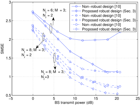
Figure 2: SMSE versus BS transmit power ($P_{T}=\|{\bf B}\|^{2}_{F}$) performance of the proposed robust design in Sec. III for the SE model. $N_{t}=8,\,6$, $M=3$, $N_{r_{1}}=N_{r_{2}}=N_{r_{3}}=2$, $L_{1}=L_{2}=L_{3}=2$, $\sigma_{n}^{2}=1$, $\sigma_{E}^{2}=0.1$. Proposed robust design in Sec. III outperforms the non-robust design in [10].

First, we consider the performance of the robust transceiver design presented in Sec. III for the stochastic CSIT error model. We consider a system with the BS transmitting $L=2$ data streams each to $M=3$ users. In Fig. 2, we present the simulated SMSE performances of the proposed robust design and those of the non-robust design proposed in [10] for different numbers of transmit antennas at the BS and receive antennas at the user terminals. Specifically, we consider three configurations: $i)$ $N_{t}=6$, $N_{r}=2$, $ii)$ $N_{t}=8$, $N_{r}=2$, and $iii)$ $N_{t}=8$, $N_{r}=3$. We use $\sigma_{E}^{2}=0.1$ in all the three configurations. From Fig. 2, it can be observed that, in all the three configurations, the proposed robust design clearly outperforms the non-robust design in [10]. Comparing the results for $N_{t}=6$ and $N_{t}=8$, we find that the difference between the non-robust design and the proposed robust design decreases when more transmit antennas are provided. A similar effect is observed for increase in number of receive antennas for fixed number of transmit antennas. It is also found that the difference between the performance of these algorithms increase as the SNR increases. This is observable in (17), where the second term shows the effect of the CSIT error variance amplified by the transmit power. In Fig. 3, we illustrate the SMSE performance as a function of different channel estimation error variances, $\sigma^{2}_{E}$, for similar system parameter settings as in Fig. 2. In Fig. 3 also, we observe that the proposed robust design performs better than the non-robust design in the presence of CSIT error; larger the estimation error variance, higher is the performance improvement due to robustification in the proposed algorithm.

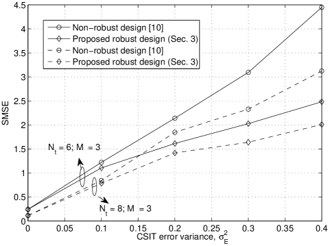
Figure 3: SMSE versus CSIT error variance ($\sigma_{E}^{2}$) performance of the proposed robust design in Sec. III for the SE model. $N_{t}=6,\,8$, $M=3$, $N_{r_{1}}=N_{r_{2}}=N_{r_{3}}=2$, $L_{1}=L_{2}=L_{3}=2$, $P_{max}=15\,\,\text{dB}$, $\sigma_{n}^{2}=1$. Larger the value of $\sigma_{E}^{2}$, higher is the performance improvement due to the proposed design in Sec. III compared to the non-robust design in [10].

Next, we present the performance of the robust transceiver designs proposed in Sec. IV for the norm-bound model of CSIT error. Figure 4 shows the SMSE performance of the proposed design in Sec. IV-A as a function of the CSIT uncertainty size, $\delta$, for the following system settings: $N_{t}=6,\,4$, $M=2$, $N_{r_{1}}=N_{r_{2}}=N_{r_{3}}=2$, $L_{1}=L_{2}=L_{3}=2$, $\delta_{1}=\delta_{2}=\delta$, $P_{max}=15\,\,\text{dB}$, and $\sigma_{n}^{2}=0.1$. It is seen that the proposed design in Sec. IV-A is able to provide improved performance compared to the non-robust transceiver design in [10], and this improvement gets increasingly better for increasing values of the CSIT uncertainty size, $\delta$. In Fig. 5, we illustrate the performance of the robust MSE-constrained design proposed in Sec. IV-B for the following set of system parameters: $N_{t}=4,\,6$, $M=2$, $N_{r_{1}}=N_{r_{2}}=2$, $L_{1}=L_{2}=2$, and $\delta_{1}=\delta_{2}=\delta=0.05,0.1$. We plot the total BS transmit power, $P_{T}=\|{\bf B}\|_{F}^{2}$, required to achieve a certain maximum allowed MSE at the user terminals, $\eta_{1}=\eta_{2}=\eta$. As expected, as the maximum allowed MSE is increased, the required total BS transmit power decreases. For comparison purposes, we have also shown the plots for the robust linear transceiver design presented in [20] for the same NBE model. It can be seen that the proposed THP transceiver design needs lesser total BS transmit power than the robust linear transceiver in [20] for a given maximum allowed MSE. The improvement in performance over robust linear transceiver is more when the maximum allowed MSE is small.

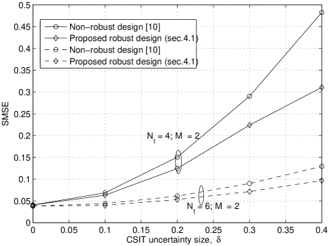
Figure 4: SMSE versus CSIT uncertainty size ($\delta$) performance of the proposed robust design in Sec. IV-A for the NBE model. $N_{t}=6,\,4$, $M=2$, $N_{r_{1}}=N_{r_{2}}=N_{r_{3}}=2$, $L_{1}=L_{2}=L_{3}=2$, $\delta_{1}=\delta_{2}=\delta$, $P_{max}=15\,\,\text{dB}$, $\sigma_{n}^{2}=0.1$. Proposed robust design in Sec. IV-A performs better than the design in [10].

Further, in Fig. 6, we present the total BS transmit power required to meet MSE constraints at user terminals for different values of CSIT uncertainty size $\delta_{1}=\delta_{2}=\delta$, for $N_{t}=4$, $M=2$, $N_{r_{1}}=N_{r_{2}}=2$, $L_{1}=L_{2}=2$, and maximum allowed MSEs $\eta_{1}=\eta_{2}=\eta=0.1,0.2,0.3$. As can be seen from Fig. 6, the proposed robust THP transceiver design in Sec. IV-B meets the desired MSE constraints with much less BS transmit power compared to the robust linear transceiver in [20]. We note that infeasibility of robust transceiver design for certain realizations of channels is an issue in robust designs with MSE constraints. In Fig. 7, we show the performance of the proposed THP transceiver design in Sec. IV-B, in terms of the fraction of channel realizations for which the design is infeasible for $N_{t}=4$, $M=2$, $N_{r_{1}}=N_{r_{2}}=2$, and different values of $\delta$ and $\eta$. It is seen that that the fraction of infeasible channel realizations in case of the proposed THP transceiver is much less compared to that in case of the linear transceiver in [20]. For example, for CSIT uncertainty size $\delta_{1}=\delta_{2}=\delta=0.08$ and user MSE $\eta_{1}=\eta_{2}=\eta=0.05$, the linear transceiver design fails to produce a feasible solution in about $44\%$ cases, whereas the proposed THP transceiver design fails only in about $24\%$ cases. In Fig. 8, we show the convergence behavior of the proposed design. The number of iterations to converge depends on the MSE constraints. Stricter MSE constraints lead to larger number of iterations to converge. For example, when the MSE constraint is $\eta=0.3$, the algorithm converges in around 6 iterations. Whereas, for $\eta=0.1$, it takes around 12 iterations to converge.

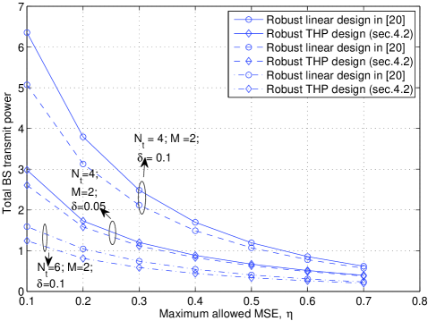
Figure 5: Total BS transmit power ($P_{T}=\|{\bf B}\|^{2}_{F}$) required as a function of maximum allowed MSE at the user terminals ($\eta_{1}=\eta_{2}=\eta$) in the proposed robust design in Sec. IV-B for the NBE model. $N_{t}=4,\,6$, $M=2$, $N_{r_{1}}=N_{r_{2}}=2$, $L_{1}=L_{2}=2$, CSIT uncertainty range $\delta_{1}=\delta_{2}=\delta=0.05,0.1$. Proposed robust THP transceiver design in Sec. IV-B requires lesser BS transmit power to meet the MSE constraints at the user terminals than the robust linear transceiver design in [20].

Finally, in Fig. 9, we present the performance of the proposed robust MSE-balancing transceiver design in Sec. IV-C for $N_{t}=4$, $M=2$, $N_{r_{1}}=N_{r_{2}}=2$, $L_{1}=L_{2}=2$, $\delta_{1}=\delta_{2}=\delta=0.02,0.1,0.15$. The min-max MSE plots as a function of total BS transmit power constraint are shown. The corresponding plots for the robust linear transceiver in [20] are also shown. The results in Fig. 9 show that, for the same BS transmit power constraint, the proposed robust design in Sec. IV-C achieves lower min-max MSE compared to the robust linear transceiver design in [20].

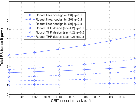
Figure 6: Total BS transmit power ($P_{T}=\|{\bf B}\|^{2}_{F}$) required as a function of CSIT uncertainty size, $\delta$, to meet MSE constraints in the proposed robust design in Sec. IV-B for the NBE model. $N_{t}=4$, $M=2$, $N_{r_{1}}=N_{r_{2}}=2$, $L_{1}=L_{2}=2$, maximum allowed MSEs $\eta_{1}=\eta_{2}=\eta=0.1,0.2,0.3$, and $\delta_{1}=\delta_{2}=\delta$. Proposed robust THP transceiver design requires lesser BS transmit power than the robust linear transceiver design in [20].

VI Conclusions

We proposed robust THP transceiver designs that jointly optimize the THP precoder and receiver filters in multiuser MIMO downlink in the presence of imperfect CSI at the transmitter. We considered these transceiver designs under SE and NBE models for CSIT errors. For the SE model, we proposed a minimum SMSE transceiver design. For the NBE model, we proposed three robust designs, namely, minimum SMSE design, MSE-constrained design, and MSE-balancing design. We presented iterative algorithms to solve these robust design problems. The iterative algorithms involved solution of sub-problems, which have either analytical solutions or can be formulated as convex optimization problems that can be solved efficiently. Through simulation results we illustrated the superior performance of the proposed robust designs compared to non-robust designs as well as robust linear transceiver designs that have been reported recently in the literature.

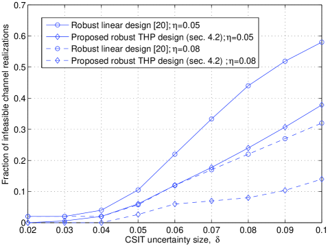
Figure 7: Fraction of infeasible channel realizations for different values of CSIT uncertainty size $\delta_{1}=\delta_{2}=\delta$ in the proposed robust design in Sec. IV-B for the NBE model. $N_{t}=4$, $M=2$, $N_{r_{1}}=N_{r_{2}}=2$, $L_{1}=L_{2}=2$, and $\eta_{1}=\eta_{2}=\eta=0.05,0.08$. Proposed robust THP transceiver design in Sec. IV-B has lesser infeasible channel realizations than the robust linear design in [20].

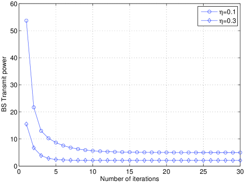
Figure 8: Convergence behavior of the proposed robust THP transceiver design in Sec. IV-B. CSIT uncertainty size $\delta_{1}=\delta_{2}=\delta=0.1$. $N_{t}=4$, $M=2$, $N_{r_{1}}=N_{r_{2}}=2$, $L_{1}=L_{2}=2$, and $\eta_{1}=\eta_{2}=\eta=0.1,0.3$.

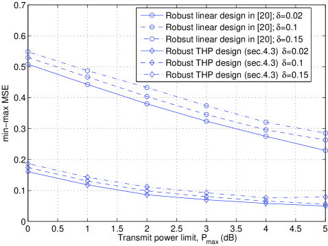
Figure 9: Min-max MSE versus total BS transmit power limit, $P_{max}$, in the proposed robust design in Sec. IV-C for the NBE model. $N_{t}=4$, $M=2$, $N_{r_{1}}=N_{r_{2}}=2$, $L_{1}=L_{2}=2$, $\delta_{1}=\delta_{2}=\delta=0.02,0.1,0.15$. Proposed robust THP transceiver design in Sec. IV-C performs better than the robust linear design in [20].

P. Ubaidulla received the B.Tech degree in Electronics and Communication Engineering from the National Institute of Technology (NIT), Calicut in 1997, and the M.E degree in Communication Engineering from NIT, Trichy in 2001. From 1998 to 1999, he was with Hindustan Petroleum Corporation as an engineer. From 2001 to 2005, he was with Central Research Laboratory, Bharat Electronics Limited, Bangalore, India, working on signal processing algorithms for radar and sonar applications. Since 2005 he has been working towards the Ph.D degree in wireless communications at the Department of Electrical Communication Engineering, Indian Institute of Science, Bangalore, India. His current research interests are in multiuser MIMO communications and robust optimization.

A. Chockalingam was born in Rajapalayam, Tamil Nadu, India. He received the B.E. (Honors) degree in Electronics and Communication Engineering from the P. S. G. College of Technology, Coimbatore, India, in 1984, the M.Tech degree with specialization in satellite communications from the Indian Institute of Technology, Kharagpur, India, in 1985, and the Ph.D. degree in Electrical Communication Engineering (ECE) from the Indian Institute of Science (IISc), Bangalore, India, in 1993. During 1986 to 1993, he worked with the Transmission R & D division of the Indian Telephone Industries Limited, Bangalore. From December 1993 to May 1996, he was a Postdoctoral Fellow and an Assistant Project Scientist at the Department of Electrical and Computer Engineering, University of California, San Diego. From May 1996 to December 1998, he served Qualcomm, Inc., San Diego, CA, as a Staff Engineer/Manager in the systems engineering group. In December 1998, he joined the faculty of the Department of ECE, IISc, Bangalore, India, where he is a Professor, working in the area of wireless communications and networking. Dr. Chockalingam is a recipient of the Swarnajayanti Fellowship from the Department of Science and Technology, Government of India. He served as an Associate Editor of the IEEE Transactions on Vehicular Technology from May 2003 to April 2007. He currently serves as an Editor of the IEEE Transactions on Wireless Communications. He served as a Guest Editor for the IEEE JSAC Special Issue on Multiuser Detection for Advanced Communication Systems and Networks. He is a Fellow of the Institution of Electronics and Telecommunication Engineers, and a Fellow of the Indian National Academy of Engineering.

References

• [1] D. Tse and P. Viswanath, Fundamentals of Wireless Communication, Cambridge University Press, 2006.
• [2] H. Bolcskei, D. Gesbert, C. B. Papadias, and A.-J. van der Veen, Space-time Wireless Systems: From Array Processing to MIMO Communications, Cambridge University Press, 2006.
• [3] Q. H. Spencer, A. L. Swindlehurst, and M. Haardt, โ€œZero-forcing methods for downlink spatial multiplexing in multiuser MIMO channels,โ€ IEEE Trans. Signal Process., vol. 52, pp. 461-471, February 2004.
• [4] K. Kusume, M. Joham, W. Utschick, and G. Bauch, โ€œEfficient Tomlinson-Harashima precoding for spatial multiplexing on flat MIMO channel,โ€ Proc. IEEE ICCโ€™2005, pp. 2021-2025, May 2005.
• [5] R. Doostnejad, T. J. Lim, and E. Sousa, โ€œJoint precoding and beamforming design for the downlink in a multiuser MIMO system,โ€ Proc. IEEE WiMobโ€™2005, pp. 153-159, August 2005.
• [6] B. Bandemer, M. Haardt, and S. Visuri, โ€œLinear MMSE multiuser MIMO downlink precoding for users with multiple antennas,โ€ Proc. IEEE PIMRCโ€™2006, pp. 1-5, September 2006.
• [7] J. Zhang, Y. Wu, S. Zhou, and J. Wang, โ€œJoint linear transmitter and receiver design for the downlink of multiuser MIMO systems,โ€ IEEE Commun. Lett., vol. 9, pp. 991-993, November 2005.
• [8] S. Shi, M. Schubert, and H. Boche, โ€œDownlink MMSE transceiver optimization for multiuser MIMO systems: Duality and sum-MSE minimization,โ€ IEEE Trans. Signal Process., vol. 55, pp. 5436-5446, November 2007.
• [9] A. Mezghani, M. Joham, R. Hunger, and W. Utschick, โ€œTransceiver design for multiuser MIMO systems,โ€ Proc. WSAโ€™2006, March 2006.
• [10] โ€”โ€”, โ€œIterative THP transceiver optimization for multiuser MIMO systems based on weighted sum-MSE minimization,โ€ Proc. IEEE SPAWCโ€™2006, July 2006.
• [11] S. Shi, M. Schubert, and H. Boche, โ€œDownlink MMSE transceiver optimization for multiuser MIMO systems: MMSE balancing,โ€ IEEE Trans. Signal Process., vol. 56, pp. 3702-3712, August 2008.
• [12] R. Doostnejad, T. J. Lim, and E. Sousa, โ€œPrecoding for the MIMO broadcast channels with multiple antennas at each receiver,โ€ Proc. CISSโ€™2005, John Hopkins University, March 2005.
• [13] N. Jindal, โ€œMIMO broadcast channels with finite rate feedback,โ€ Proc. IEEE GLOBECOMโ€™2005, November 2005.
• [14] R. Hunger, F. Dietrich, M. Joham, and W. Utschick, โ€œRobust transmit zero-forcing filters,โ€ Proc. ITG Workshop on Smart Antennas, Munich, pp. 130-137, March 2004.
• [15] M. B. Shenouda and T. Davidson, โ€œConvex conic formulations of robust downlink precoder design with quality of service constraints,โ€ IEEE Jl. Sel. Topic Signal Proc,, vol. 1, pp. 714-724, December 2007.
• [16] M. Biguesh, S. Shahbazpanahi, and A. B. Gershman, โ€œRobust downlink power control in wireless cellular systems,โ€ EURASIP Jl. on Wireless Commun. and Networking, vol. 2, pp. 261โ€“272, 2004.
• [17] M. Payaro, A. Pascual-Iserte, and M. A. Lagunas, โ€œRobust power allocation designs for multiuser and multi-antenna downlink communication systems through convex optimization,โ€ IEEE Jl. Sel. Areas Commun., vol. 25, pp. 1392-1401, September 2007.
• [18] N. Vucic and H. Boche, โ€œRobust QoS-constrained optimization of downlink multiuser MISO systems,โ€ IEEE Trans. Signal Process., vol. 57, pp. 714-725, February 2009.
• [19] M. B. Shenouda and T. Davidson, โ€œNon-linear and linear broadcasting with QoS requirements: Tractable approaches for bounded channel uncertainties,โ€ to appear in IEEE Trans. Signal Process., arXiv:0712.1659v1 [cs.IT] 11 Dec 2007.
• [20] N. Vucic, H. Boche, and S. Shi, โ€œRobust transceiver optimization in downlink multiuser MIMO systems with channel uncertainty,โ€ Proc. IEEE ICCโ€™2008, May 2008.
• [21] A. Pascual-Iserte, D. P. Palomar, A. I. Perez-Neira, and M. A. Lagunas, โ€œA robust maximin approach for MIMO communications with imperfect channel state information based on convex optimization,โ€ IEEE Trans. Signal Process., vol. 54, pp. 346-360, January 2006.
• [22] R. F. H. Fischer, Precoding and Signal Shaping for Digital Transmission, John Wiley & Sons, 2002.
• [23] S. Boyd and L. Vandenberghe, Convex Optimization, Cambridge University Press, 2004.
• [24] J. Sturm, โ€œUsing SeDuMi 1.02, a MATLAB toolbox or optimization over symmetric cones,โ€ Optimization Methods and Software, vol. 11, pp. 625-653, 1999.
• [25] A. Ben-Tal and A. Nemirovsky, โ€œSelected topics in robust optimization,โ€ Math. Program., vol. 112, pp. 125-158, February 2007.
• [26] R. A. Horn and C. R. Johnson, Matrix Analysis, Cambridge University Press, 1985.
• [27] Y. C. Eldar, A. Ben-Tal, and A.Nemirovski, โ€œRobust mean-squared error estimation in the presence of model uncertainties,โ€ IEEE Trans. Signal Process., vol. 53, pp. 161-176, January 2005.
• [28] W. Yu and T. Lan, โ€œTransmitter optimization for multi-antenna downlink with per-antenna power constraints,โ€ IEEE Trans. Signal Process., vol. 55, pp. 2646-2660, June 2007.
• [29] A. Wiesel, Y. C. Eldar, and Shamai, โ€œLinear precoder via conic optimization for fixed MIMO receivers,โ€ IEEE Trans. Signal Process., vol. 52, pp. 161-176, January 2006.
• [30] M. Schubert and H. Boche, โ€œSolution of multiuser downlink beamforming problem with individual SINR constraints,โ€ IEEE Trans. Veh. Technol., vol. 53, pp. 18-28, January 2004.
• [31] โ€”โ€”, โ€œIterative multiuser uplink and downlink beamforming under SINR constraints,โ€ IEEE Trans. Signal Process., vol. 53, pp. 2324-2334, July 2005.
• [32] M. B. Shenouda and T. N. Davidson, โ€œLinear matrix inequality formulations of robust QoS precoding for broadcast channels,โ€ Proc. CCECEโ€™2007, pp. 324-328, April 2007.
• [33] H. Boche and M. Schubert, โ€œA general theory for SIR balancing,โ€ EURASIP Jl. on Wireless Commun. and Networking, pp. 1-18, February 2006.