Precise dipole model analysis of diffractive DIS

Abstract

We analyse the newest diffractive deep inelastic scattering data from HERA using the dipole model approach. We find a reasonable good agreement between the predictions and the data although the region of small values of a kinematic variable $\beta$ needs refinement. A way to do this is to consider an approach with diffractive parton distributions evolved with the DGLAP evolution equations.

1 Introduction

The most promissing QCD based approach to DIS diffraction is formulated by a systematic formation of the diffractive state from parton components of the light cone virtual photon wave function, projected onto the color singlet state. The lowest order states are formed by a quark-antiquark pair $(q\overline{q}))$ and a $q\overline{q}$–gluon system while higher order states contain aditional $q\overline{q}$ pairs and gluons $g$. We will concentrate on the first two components since they can be viewed in the configuration space conjugate to parton transverse momentum as quark or gluon color dipoles. This is the basis of the dipole models which have to be supplemented by the way the dipoles interact with the proton, which is described by the scattering amplitude $N(r,b)$. In this analysis, we consider two important parameterisations of the dipole scattering amplitude, called GBW [5] and CGC [10], in which parton saturation results are built in. Here we present a precise comparison of the results of the dipole models with these two parameterisations with the newest data from HERA on the combination of the diffractive structure functions, obtained by the ZEUS [4] collaboration.

1.1 Diffractive structure functions in dipole models

In the dipole approach to DDIS, the diffractive structure function $F_{2}^{D}$ is a sum of components corresponding to different diffractive final states produced by transversely $(T)$ and longitudinally $(L)$ polarised virtual photon [14]. We consider two component diffractive final state which is built from $q\overline{q}$ pair from transverse and longitudinal photon and $q\overline{q}g$ system from transverse photon. Thus, the structure function is given as a sum

$$F_{2}^{D}(x_{{I\!\!P}},\beta,Q^{2})=F_{T}^{(q\overline{q})}+F_{L}^{(q\overline{q})}+F_{T}^{(q\overline{q}g)}$$ (1)

where the kinematic variables depend on diffractive mass $M$ and center-of-mass energy of the $\gamma^{*}p$ system $W$ through

$$x_{{I\!\!P}}=\frac{M^{2}+Q^{2}}{W^{2}+Q^{2}}\,,~{}~{}~{}~{}~{}~{}~{}~{}~{}~{}\beta=\frac{Q^{2}}{Q^{2}+M^{2}}$$ (2)

while the standard Bjorken variable $x=x_{{I\!\!P}}\beta$. The dependence of $F_{2}^{D}$ on the momentum transfer $t=(p-p^{\prime})^{2}$ is integrated out. The $q\overline{q}$ components from transversely and longitudinally polarised photons are given by

$$x_{{I\!\!P}}F_{T}^{(q\overline{q})}\!\! = \!\!\frac{3Q^{4}}{64\/\pi^{4}\beta B_{d}}\,\sum_{f}e_{f}^{2}\int_{z_{f}}^{1/2}dz\,z(1-z)$$ (3)

$$\times \left\{[z^{2}+(1-z)^{2}]\,Q^{2}_{f}\,\phi_{1}^{2}\,+\,m_{f}^{2}\,\phi_{0}^{2}\right\}~{}~{}~{}~{}~{}~{}~{}~{}$$

$$x_{{I\!\!P}}F_{L}^{(q\overline{q})}\!\! = \!\!\frac{3Q^{6}}{16\/\pi^{4}\beta B_{d}}\,\sum_{f}e_{f}^{2}\int_{z_{f}}^{1/2}dz\,z^{3}(1-z)^{3}\,\phi_{0}^{2}$$ (4)

where $f$ denotes quark flavours, $m_{f}$ is quark mass and the diffractive slope $B_{d}$ in the denominator results from the $t$-integration of the structure functions, assuming an exponential form for this dependence. From HERA data, $B_{d}=6~{}{\textrm{G}eV}^{-2}$. The variables

$$z_{f}={\textstyle{\frac{1}{2}}}(1-\sqrt{1-4m_{f}^{2}/M^{2}})\,,~{}~{}~{}~{}Q^{2}_{f}=z(1-z)Q^{2}+m_{f}^{2}$$ (5)

and the functions $\phi_{i}$ take the following form for $i=0,1$

$$\phi_{i}=\int_{0}^{\infty}drrK_{i}\!\left(Q_{f}r\right)J_{i}\!\left(k_{f}r\right)\hat{\sigma}(x_{{I\!\!P}},r)$$ (6)

where $k_{f}=\sqrt{z(1-z)M^{2}-m_{f}^{2}}$ is the quark transverse momentum while $K_{i}$ and $J_{i}$ are the Bessel functions. The lower integration limit $z_{f}$ in eqs. (3) and (4) corresponds to a minimal value of $z$ for which the diffractive state with mass $M$ can be produced. In such a case $k_{f}=0$. At the threshold for the massive quark production $M^{2}=4m_{f}^{2}$ and $z_{f}=1/2$, leading to $F_{T,L}^{(q\overline{q})}=0$. For massless quarks $z_{f}=0$. The $q\overline{q}g$ diffractive component from transverse photons, computed for massless quarks is given by

$$x_{{I\!\!P}}F_{T}^{(q\overline{q}g)} = \frac{81\beta\alpha_{s}}{512\pi^{5}B_{d}}\;\sum_{f}e_{f}^{2}\int_{\beta}^{1}\frac{dz}{(1-z)^{3}}$$ (7)

$$\times \left[\left(1-\frac{\beta}{z}\right)^{2}+\left(\frac{\beta}{z}\right)^{2}\right]$$

$$\times \int_{0}^{(1-z)Q^{2}}dk^{2}\log\left(\frac{(1-z)Q^{2}}{k^{2}}\right)\phi_{2}^{2}$$

where the function $\phi_{2}$ takes to form

$$\phi_{2}=k^{2}\int_{0}^{\infty}dr\,r\,K_{2}\!\left(\sqrt{\frac{z}{1-z}}kr\right)\,J_{2}(kr)\,\hat{\sigma}(x_{{I\!\!P}},r)$$ (8)

with $K_{2}$ and $J_{2}$ are the Bessel functions. In papers [15, 7], formula (7) was computed with two gluons exchanged between the diffractive system and the proton. Then, the two gluon exchange interaction was substituted by the dipole cross section $\hat{\sigma}=\hat{\sigma}(x_{{I\!\!P}},r)$ for the $q\overline{q}$ dipole interaction with the proton. For example, for the GBW parameterisation of the dipole cross section [15], which we discuss in the next section, is given by

$$\hat{\sigma}\equiv\hat{\sigma}_{q\overline{q}}=\sigma_{0}\left(1-{\mbox{{e}}}^{-r^{2}Q_{s}^{2}/4}\right)\,.$$ (9)

However, the $q\overline{q}g$ system was computed in the approximation when parton transverse momenta fulfil the condition $k_{Tq}\approx k_{T\overline{q}}\gg k_{Tg}$. Thus, in the large $N_{c}$ approximation, it can be treated as a gluonic color dipole $gg$. Such a dipole interacts with the relative color factor $C_{A}/C_{F}$ with respect to the $q\overline{q}$ dipole. Therefore, the two gluon exchange formula should be eikonalized with this color factor absorbed into the exponent. For the GBW parameterisation, this leads to the following gluon dipole cross section in eq. (8)

$$\hat{\sigma}\equiv\hat{\sigma}_{gg}=\sigma_{0}\left(1-{\mbox{{e}}}^{-(C_{A}/C_{F})r^{2}Q_{s}^{2}/4}\right)\,.$$ (10)

In such a case, the color factor $C_{A}/C_{F}=9/4$ (for $N_{c}=3$) disappears from the normalisation of the scattering amplitude and we have to rescale the structure function in the following way

$$F_{T}^{(q\overline{q}g)}~{}\to~{}\frac{1}{(C_{A}/C_{F})^{2}}\,F_{T}^{(q\overline{q}g)}\,.$$ (11)

By the comparison with HERA data, we will show in the next section that the latter possibility is more appropriate for the data description. In this analysis we considered two parameterisations: GBW from [5] and CGC parameterisation with heavy quarks [10, 8] see our paper [17] for more details.

2 Diffractive charm quark production

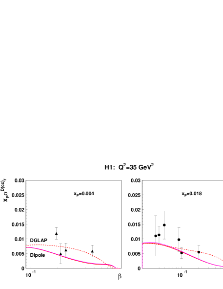
Figure 1: A comparison of the collinear factorisation predictions with the GBW and CGC gluon distributions (solid lines) with the HERA data on the open diffractive charm production

In the diffractive scattering heavy quarks are produced in quark-antiquark pairs, $c\overline{c}$ and $b\overline{b}$ for charm and bottom, respectively. Such pairs can be produced provided that the diffractive mass of is above the quark pair production threshold

$$M^{2}=Q^{2}\left(\frac{1}{\beta}-1\right)>4m_{c,b}^{2}$$ (12)

In the lowest order the diffractive state consist only the $c\overline{c}$ or $b\overline{b}$ pair. In the forthcoming we consider only charm production since bottom production is negligible.The corresponding contributions to $F_{2}^{D}$ are given by eqs. (3) and (4) with one flavour component. For example, for charm production from transverse photons we have

$$x_{{I\!\!P}}F_{T}^{(c\overline{c})}\!\! = \!\!\frac{3Q^{4}e_{c}^{2}}{64\/\pi^{4}\beta B_{d}}\int_{z_{c}}^{1/2}dz\,z(1-z)$$ (13)

$$\times \left\{[z^{2}+(1-z)^{2}]\,Q^{2}_{c}\,\phi_{1}^{2}\,+\,m_{c}^{2}\,\phi_{0}^{2}\right\}$$

where $m_{c}$ and $e_{c}$ are charm quark mass and electric charge, respectively. The minimal value of diffractive mass equals: $M^{2}_{min}=4m_{c}^{2}$, thus the maximal value of $\beta$ is given by

$$\beta_{max}=\frac{Q^{2}}{Q^{2}+4m_{c}^{2}}\,.$$ (14)

In such a case, $z_{c}=1/2$ in Eq., for $x_{{I\!\!P}}F_{T}^{(c\overline{c})}$ and $F_{T,L}^{(c\overline{c})}=0$ for $\beta>\beta_{max}$. Figure 1 shows the collinear factorisation predictions for the diffractive charm production confronted with the new HERA data [3] on the charm component of the reduced cross section. The solid curves, which are barley distinguishable, correspond to the result with the GBW and CGC parameterisations of the diffractive gluon distributions. The dashed lines are computed for the gluon distribution from a fit to the H1 data [16] based on the DGLAP equations.

3 Comparison with the HERA data

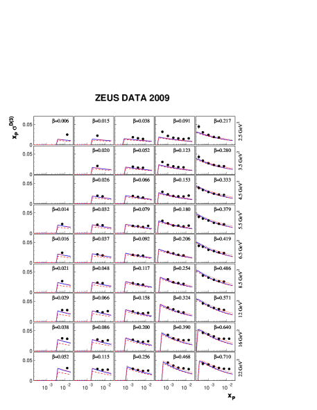
Figure 2: A comparison of $\sigma_{r}^{D}$ from the two considered dipole models with the newest ZEUS collaboration data [11]. The solid lines correspond to the GBW parameterisation of the dipole cross section with the color factor modifications (10) and (11), while the dotted lines correspond to the CGC parameterisation. The dashed lines show the results without the charm contribution.

Figure 2 shows a comparison of the dipole model predictions with the ZEUS collaboration data [11] on the reduced cross section

$$\sigma_{r}^{D}=F_{2}^{D}-\frac{y^{2}}{1+(1-y)^{2}}F_{L}^{D}\,.$$ (15)

We included the charm contribution in the above structure functions. The solid lines correspond to the GBW parameterisation of the dipole cross section with the color factor modifications (10) and (11) of the $q\overline{q}g$ component, while the dashed lines are obtained from the CGC parameterisation. We see that the two sets of curves are barely distinguishable The color factor modification of the $q\overline{q}g$ component in the GBW parameterisation is necessary since the curves without such a modification significantly overshoot the data (by a factor of two or so) in the region of small $\beta$ where the ${q\overline{q}g}$ component dominates. The comparison of the predictions with the data also reveals a very important aspect of the three component dipole model (1). In the small $\beta$ region, the curves are systematically below the data points, which effect may be attributed to the lack of higher order components in the diffractive state, i.e. with more than one gluon or $q\overline{q}$ pair. This is also seen for the H1 collaboration data [2] shown in our last paper [17]. In our analysis we also computed the gluon distributions respectively for the GBW parameterisation with the color factor modification and for the CGC parameterisation. We compare them with the gluon distributions found in the DGLAP fit with higher twist to the recent H1 data [16] and use it for the computation of the charm contribution to $F_{2}^{D}$, see our last work [17].

4 Summary

We presented a comparison of the dipole model results with the GBW and CGC parameterisations on the diffractive structure functions with the HERA data. The three component model with the $q\overline{q}$ and $q\overline{q}g$ diffractive states describe reasonable well the recent data. However, the region of small values of $\beta$ needs some refinement by considering components with more gluons and $q\overline{q}$ pairs in the diffractive state. This can be achieved in the DGLAP based approach which sums partonic emissions in the diffractive state in the transverse momentum ordering approximation. It is also important that the charm contribution, described in Sec. 2, is added into the analysis. Without this contribution the comparison would be much worse than that shown here.

5 Bibliography

References

-
[1]
Slides:
http://indico.cern.ch/contributionDisplay.py?contribId=114&sessionId=186&confId=53294 - [2] H1, A. Aktas et al., Eur. Phys. J. C48, 715 (2006), [hep-ex/0606004].
- [3] H1, A. Aktas et al., Eur. Phys. J. C50, 1 (2007), [hep-ex/0610076].
- [4] ZEUS, S. Chekanov et al., Nucl. Phys. B800, 1 (2008), [0802.3017].
- [5] K. Golec-Biernat and M. Wusthoff, Phys. Rev. D59, 014017 (1999), [hep-ph/9807513].
- [6] E. Iancu, K. Itakura and S. Munier, Phys. Lett. B590, 199 (2004), [hep-ph/0310338].
- [7] K. Golec-Biernat and M. Wusthoff, Phys. Rev. D60, 114023 (1999), [hep-ph/9903358].
- [8] C. Marquet, Phys. Rev. D76, 094017 (2007), [0706.2682].
- [9] H. Kowalski, L. Motyka and G. Watt, Phys. Rev. D74, 074016 (2006), [hep-ph/0606272].
- [10] G. Soyez, Phys. Lett. B655, 32 (2007), [0705.3672].
- [11] ZEUS, S. Chekanov et al., 0812.2003.
- [12] J. Bartels, K. Golec-Biernat and H. Kowalski, Phys. Rev. D66, 014001 (2002), [hep-ph/0203258].
- [13] V. P. Goncalves and M. V. T. Machado, Phys. Lett. B588, 180 (2004), [hep-ph/0401104].
- [14] J. Bartels, J. R. Ellis, H. Kowalski and M. Wusthoff, Eur. Phys. J. C7, 443 (1999), [hep-ph/9803497].
- [15] M. Wusthoff, Phys. Rev. D56, 4311 (1997), [hep-ph/9702201].
- [16] K. J. Golec-Biernat and A. Luszczak, Phys. Rev. D76, 114014 (2007), [0704.1608].
- [17] K. J. Golec-Biernat and A. Luszczak, Phys. Rev. D79, 114010 (2009), [0812.3090].