A Fast Algorithm for the Constrained Formulation of Compressive Image Reconstruction and Other Linear Inverse Problems

Abstract

Ill-posed linear inverse problems (ILIP), such as restoration and reconstruction, are a core topic of signal/image processing. A standard approach to deal with ILIP uses a constrained optimization problem, where a regularization function is minimized under the constraint that the solution explains the observations sufficiently well. The regularizer and constraint are usually convex; however, several particular features of these problems (huge dimensionality, non-smoothness) preclude the use of off-the-shelf optimization tools and have stimulated much research. In this paper, we propose a new efficient algorithm to handle one class of constrained problems (known as basis pursuit denoising) tailored to image recovery applications. The proposed algorithm, which belongs to the category of augmented Lagrangian methods, can be used to deal with a variety of imaging ILIP, including deconvolution and reconstruction from compressive observations (such as MRI). Experiments testify for the effectiveness of the proposed method.

Index Terms—  Optimization, inverse problems, image reconstruction/restoration, compressive sensing, total variation, tight frames.

1 Introduction

1.1 Problem Formulation

Linear inverse problems constitute one of the central themes of signal/image processing. In this class of problems, a noisy indirect observation ${\bf y}$, of an original signal ${\bf x}$, is modeled as

$${\bf y}={\bf B}{\bf x}+{\bf n},$$ (1)

where ${\bf B}$ is the matrix representation of the direct operator and ${\bf n}$ is noise. In the sequel, we denote by $n$ the dimension of ${\bf x}$, thus ${\bf x}\in\mathbb{R}^{n}$, while ${\bf y}\in\mathbb{R}^{m}$. In the classical problem of image deblurring/deconvolution, ${\bf B}$ is the matrix representation of a convolution operator. In other reconstruction problems, ${\bf B}$ represents some linear direct operator, such as of tomographic projections (Radon transform) or a partially observed (e.g., Fourier) transform (as in compressive MRI [19]).

Usually, the problem of estimating ${\bf x}$ from ${\bf y}$ is ill-posed (e.g., if $m<n$), thus requiring some sort of regularization. In the presence of noise, a natural criterion to infer ${\bf x}$ from ${\bf y}$ has the form [7, 20]

$$\min_{{\bf x}}\phi(\bf x)\hskip 14.22636pt\mbox{subject to}\hskip 7.11317pt\|{\bf B}{\bf x}-{\bf y}\|_{2}\leq\varepsilon,$$ (2)

where $\phi:\mathbb{R}^{n}\rightarrow\bar{\mathbb{R}}$ is the the regularizer and $\varepsilon\geq 0$ a parameter which depends on the noise variance. In the case where $\phi({\bf x})=\|{\bf x}\|_{1}$, the above problem is usually known as basis pursuit denoising (BPD) [8]. The basis pursuit (BP) problem is the particular case of (2) for $\varepsilon=0$. In recent years, an explosion of interest in problems of the form (2) was sparked by the emergence of compressive sensing (CS) [5], [10]. The theory of CS provides conditions (on matrix ${\bf B}$ and the degree of sparseness of the original ${\bf x}$) under which a solution of (2) is an optimal (in some sense) approximation to the “true” ${\bf x}$.

In most image recovery and CS problems, the regularizer $\phi$ is convex but non-smooth; typical examples are the total variation (TV) [5], [23] and $\ell_{1}$ norms. Problem (2) is thus convex, but the very high dimension (usually $\geq 10^{4}$) of ${\bf x}$ and ${\bf y}$ precludes the direct application of off-the-shelf optimization algorithms. This difficulty is further amplified by the fact that matrix ${\bf B}$ only “exists” as an operator; i.e., there are efficient algorithms to compute products of ${\bf B}$ (or ${\bf B}^{T}$) by some vector (image), but it is highly impractical to extract and manipulate individual blocks, rows, or columns of this matrix.

1.2 Previous Work

Most state-of-the-art methods for dealing with linear inverse problems, under convex, non-smooth regularizers (namely, TV and $\ell_{1}$), consider, rather than (2), the unconstrained problem

$$\min_{{\bf x}}\frac{1}{2}\|{\bf B\,x}-{\bf y}\|_{2}^{2}+\tau\,\phi({\bf x}),$$ (3)

where $\tau\in\mathbb{R}_{+}$ is the so-called regularization parameter. Of course, problems (2) and (3) are equivalent, in the following sense: for any $\varepsilon$ such that problem (2) is feasible, a solution of (2) is either the null vector, or else is a solution of (3), for some $\tau$ [15].

The currently fastest (publicly available) algorithms for solving (3), include: gradient projection for sparse reconstruction (GPSR) [15]; fast iterative shrinkage/thresolding algorithm (FISTA) [1]; two-step IST (TwIST) [2]; and sparse reconstruction by separable approximation (SpaRSA) [28]. These methods were shown to be considerably faster than earlier methods, including $l1\verb=_=ls$ [18] and the codes in the $\ell_{1}$-magic (http://www.l1-magic.org) and the SparseLab (http://sparselab.stanford.edu) toolboxes. Very recently, we have introduced a new algorithm, called SALSA (split augmented Lagrangian shrinkage algorithm); experiments on a set of standard image recovery problems show that SALSA is faster than GPSR, TwIST, FISTA, and SpaRSA [13].

Although it is usually easier/simpler to solve an unconstrained problem than a constrained one, formulation (2) has an important advantage: parameter $\varepsilon$ has a clear meaning (it is proportional to the noise variance) and is much easier to set than parameter $\tau$ in (3). Of course, one may solve (2) by using one of the algorithms mentioned in the previous paragraph to solve (3) and searching for the “correct” value of $\tau$ that makes (3) equivalent to (2). Clearly, this is not efficient, as it involves solving many instances of (3). Obtaining fast algorithms for solving (2) is thus an important research front.

There are few efficient algorithms to solve (2) in an image recovery context: ${\bf x}$ and ${\bf y}$ of dimension $\geq 10^{4}$ (often $\geq 10^{6}$), ${\bf B}$ representing an operator, and $\phi$ a convex, non-smooth function. A notable exception is the recent SPGL1 [26], which (as its name implies) is specifically designed for $\ell_{1}$ regularization ($\phi({\bf x})=\|{\bf x}\|_{1}$). Other methods for solving problems with the form (2), for $\phi$ equal to the $\ell_{1}$ or TV norms, are available in the $\ell_{1}$-magic package; however, as shown in [26], those methods are quite inefficient for large problems. General purpose methods, such as those in the SeDuMi package (http://sedumi.ie.lehigh.edu), are simply not applicable when ${\bf B}$ is not an actual matrix, but an operator.

The Bregman iterative algorithm (BIA) was recently proposed to solve (2) with $\varepsilon=0$, but is not directly applicable when $\varepsilon>0$ [29]. To deal with the case of $\varepsilon>0$, it was suggested that the BIA for $\varepsilon=0$ is used and stopped when $\|{\bf B}{\bf x}-{\bf y}\|_{2}\leq\varepsilon$ [4], [29]. Clearly, that approach is not guaranteed to find a good solution, since it depends strongly on the initialization; e.g., if the algorithm starts at a feasible point, it will immediately stop, although the point may be far from a minimizer of $\phi$.

1.3 Proposed Approach

In this paper, we introduce an algorithm for solving optimization problems of the form (2). The basic ingredients are the following: the original constrained problem (2) is transformed into an unconstrained one by using an indicator function of the feasible set; the resulting unconstrained problem is transformed into a different constrained problem, by the application of a variable splitting operation; finally, the obtained constrained problem is attacked with an augmented Lagrangian (AL) scheme [22], which is a variant of the alternating direction method of multipliers (ADMM) [11]. Since (as SALSA), the proposed method uses variable splitting and AL optimization, we call it C-SALSA (for constrained-SALSA).

The resulting algorithm is more general than SPGL1, in the sense that it can be used with any convex regularizer $\phi$ for which the corresponding Moreau proximity operator [9], defined as

$$\mbox{\boldmath$\Psi$}_{\tau\phi}({\bf y})=\arg\min_{{\bf x}}\frac{1}{2}\|{\bf x}-{\bf y}\|_{2}^{2}+\tau\phi({\bf x}),$$ (4)

has closed form or can be efficiently computed. Below, we will show examples of C-SALSA where ${\bf x}$ is an image, $\phi$ is the TV norm [23], and $\mbox{\boldmath$\Psi$}_{\tau\phi}$ is computed using Chambolle’s algorithm [6]. Another classical choice is $\phi({\bf x})=\|{\bf x}\|_{1}$, which leads to $\mbox{\boldmath$\Psi$}_{\tau\phi}({\bf y})=\mbox{soft}({\bf y},\tau)$, where $\mbox{soft}(\cdot,\tau)$ denotes the component-wise application of the soft-threshold function $y\mapsto\mbox{sign}(y)\max\{|y|-\tau,0\}$.

C-SALSA is experimentally shown to efficiently solve image recovery problems of the form (2), such as MRI reconstruction from CS-type partial Fourier observations using TV regularization. Moreover, C-SALSA is also shown to be faster than SPGL1 in wavelet-based image deconvolution problems under $\ell_{1}$ regularization.

The paper is organized as follows. Section 2 briefly reviews variable splitting and ADMM. Section 3 contains the derivation leading to C-SALSA. Section 4 reports experimental results, and Section 5 ends the paper with a few remarks and pointers to future work.

2 Variable Splitting and ADMM

Consider an unconstrained optimization problem

$$\min_{{\bf u}\in\mathbb{R}^{n}}f_{1}({\bf u})+f_{2}\left({\bf G}{\bf u}\right),$$ (5)

where ${\bf G}\in\mathbb{R}^{d\times n}$. Variable splitting (VS) is a simple procedure that consists in creating new variables, say ${\bf v}$ and ${\bf w}$, to serve as the argument of each of the terms, $f_{1}$ and $f_{2}$, under the constraints that ${\bf w}={\bf u}$ and ${\bf v}={\bf G}{\bf u}$, that is,

$${\displaystyle\min_{{\bf u},{\bf w}\in\mathbb{R}^{n},\,{\bf v}\in\mathbb{R}^{d}}}\;\;f_{1}({\bf w})+f_{2}({\bf v}),\hskip 17.07182pt\mbox{subject to}\hskip 8.5359pt\begin{array}[t]{l}{\bf w}={\bf u}\\ {\bf v}={\bf G}{\bf u}.\end{array}$$ (6)

Problem (6) is clearly equivalent to the unconstrained problem (5). The rationale behind VS is that it may be easier to solve the constrained problem (6) than to solve its unconstrained counterpart (5). It is important to stress that the VS in (6) is not the one commonly used, where only variable ${\bf v}$ is created; however, as shown below, the proposed VS will lead to a very effective algorithm.

Other variants of VS were recently used in several image processing problems: in [27], it was used to obtain a fast TV-based algorithm; in [3], it was used to handle problems with compound regularization. VS also underlies the recent split-Bregman methods [16], but there the splitting is different and with a different goal.

Using an augmented Lagrangian (AL) approach to handle problem (6) leads to the following algorithm, also known as the method of multipliers (MM) [17], [24] (see also [13], for details):

$$\left({\bf u}_{k+1},{\bf v}_{k+1},{\bf w}_{k+1}\right) \in \arg\min_{{\bf u},{\bf v},{\bf w}}\;\left\{f_{1}({\bf w})+f_{2}({\bf v})+\rule[-5.69046pt]{0.0pt}{11.38092pt}\right.$$

$$\left.\rule[-5.69046pt]{0.0pt}{11.38092pt}\frac{\mu_{1}}{2}\|{\bf G}{\bf u}-{\bf v}-{\bf b}_{k}\|_{2}^{2}+\frac{\mu_{2}}{2}\|{\bf u}-{\bf w}-{\bf c}_{k}\|_{2}^{2}\right\}$$ (7)

$${\bf b}_{k+1} = {\bf b}_{k}+{\bf G}{\bf u}_{k+1}-{\bf v}_{k+1}$$ (8)

$${\bf c}_{k+1} = {\bf c}_{k}+{\bf u}_{k+1}-{\bf w}_{k+1}.$$ (9)

Problem (7) is not trivial since it involves non-separable quadratic as well as non-smooth terms. Replacing (7) by the alternating minimization with respect to each vector leads to a variant of the so-called alternating direction method of multipliers (ADMM) [11]:

• Set $k=0$, choose $\mu_{1},\mu_{2}>0$, ${\bf v}_{0}$, ${\bf w}_{0}$, ${\bf b}_{0}$, and ${\bf c}_{0}.$

• repeat

• ${\bf u}_{k+1}\leftarrow{\displaystyle\arg\min_{{\bf u}}}\frac{\mu_{1}}{\mu_{2}}\|{\bf G}{\bf u}\!-\!{\bf v}_{k}\!-\!{\bf b}_{k}\|_{2}^{2}+\|{\bf u}\!-\!{\bf w}_{k}\!-{\bf c}_{k}\|_{2}^{2}$

• ${\bf v}_{k+1}\leftarrow{\displaystyle\arg\min_{{\bf v}}}f_{2}({\bf v})+\frac{\mu_{1}}{2}\|{\bf G}{\bf u}_{k+1}-{\bf v}-{\bf b}_{k}\|_{2}^{2}$

• ${\bf w}_{k+1}\leftarrow{\displaystyle\arg\min_{{\bf w}}}f_{1}({\bf w})+\frac{\mu_{2}}{2}\|{\bf w}-{\bf u}_{k+1}-{\bf c}_{k}\|_{2}^{2}$

• ${\bf b}_{k+1}\leftarrow{\bf b}_{k}+{\bf Gu}_{k+1}-{\bf v}_{k+1}$

• ${\bf c}_{k+1}\leftarrow{\bf c}_{k}+{\bf u}_{k+1}-{\bf w}_{k+1}$

• $k\leftarrow k+1$

• until stopping criterion is satisfied.

The proof of convergence in [11] applies to a different variant of ADMM, which results from a different splitting. However, it is possible to show that this version can still be written as a standard ADMM and satisfies the conditions of the convergence theorem [12].

3 Proposed Method

3.1 Reformulation of the Problem

The feasible set in problem (2) is the ellipsoid

$$E(\varepsilon,{\bf B},{\bf y})=\{{\bf x}\in\mathbb{R}^{n}:\|{\bf B\,x}-{\bf y}\|_{2}\leq\varepsilon\},$$ (10)

possible infinite in some directions. Problem (2) can be written as an unconstrained (discontinuous) problem,

$$\min_{{\bf x}}\;\phi({\bf x})+\iota_{E(\varepsilon,{\bf I},0)}({\bf Bx-y}),$$ (11)

where $\iota_{S}:\mathbb{R}^{m}\rightarrow\bar{\mathbb{R}}$ denotes the indicator function of set $S\subset\mathbb{R}^{m}$,

$$\iota_{S}({\bf s})=\left\{\begin{array}[]{ll}0,&\text{if }{\bf s}\in S\\ +\infty,&\text{if }{\bf s}\notin S.\end{array}\right.$$ (12)

Notice that $E(\varepsilon,{\bf I},0)$ is simply an $\varepsilon$-radius Euclidean ball centered at the origin of $\mathbb{R}^{m}$.

Since problem (11) clearly has the form (5), its VS-based constrained optimization reformulation is

$${\displaystyle\min_{{\bf u},{\bf w}\in\mathbb{R}^{n},{\bf v}\in\mathbb{R}^{m}}}\;\phi({\bf w})+\iota_{E(\varepsilon,{\bf I},0)}({\bf v}),\hskip 11.38092pt\mbox{s. t.}\hskip 4.26773pt\begin{array}[t]{l}{\bf u}={\bf w}\\ {\bf v}={\bf Bu-y}.\end{array}$$ (13)

3.2 Application of ADMM

Performing the adequate translations (which are clear from comparing (6) with (13)), the ADMM becomes the proposed C-SALSA.

• Set $k=0$, choose $\mu_{1},\mu_{2}>0$, ${\bf v}_{0}$, ${\bf w}_{0}$, ${\bf b}_{0}$, and ${\bf c}_{0}.$

• repeat

• ${\bf u}^{\prime}\leftarrow{\bf w}_{k}+{\bf c}_{k}$

• ${\bf u}^{\prime\prime}\leftarrow{\bf y}+{\bf v}_{k}+{\bf b}_{k}$

• ${\bf u}_{k+1}\leftarrow{\displaystyle\arg\min_{{\bf u}}}\;\frac{\mu_{1}}{\mu_{2}}\|{\bf B\,u}-{\bf u}^{\prime\prime}\|_{2}^{2}+\|{\bf u}-{\bf u}^{\prime}\|_{2}^{2}$

• ${\bf v}^{\prime}\leftarrow{\bf Bu}_{k+1}-{\bf y}-{\bf b}_{k}$

• ${\bf v}_{k+1}\leftarrow{\displaystyle\arg\min_{{\bf v}}}\;\iota_{E(\varepsilon,{\bf I},0)}({\bf v})+\frac{\mu_{1}}{2}\|{\bf v}-{\bf v}^{\prime}\|_{2}^{2}$

• ${\bf w}^{\prime}\leftarrow{\bf u}_{k+1}+{\bf c}_{k}$

• ${\bf w}_{k+1}\leftarrow{\displaystyle\arg\min_{{\bf w}}}\;\phi({\bf w})+\frac{\mu_{2}}{2}\|{\bf w}-{\bf w}^{\prime}\|_{2}^{2}$

• ${\bf b}_{k+1}\leftarrow{\bf b}_{k}+{\bf Bu}_{k+1}-{\bf y}-{\bf v}_{k+1}$

• ${\bf c}_{k+1}\leftarrow{\bf c}_{k}+{\bf u}_{k+1}-{\bf w}_{k+1}$

• $k\leftarrow k+1$

• until stopping criterion is satisfied.

A key feature of C-SALSA is that the cost of each iteration is $O(n\log n)$, as confirmed by the following observations. Lines 3, 4, 8, 11, and 12 simply involve adding vectors or scalars, thus have $O(n)$ or $O(1)$ cost. Line 5 consists in minimizing a strictly convex quadratic function, leading (with $\alpha=\mu_{1}/\mu_{2}$) to

$${\bf u}_{k+1}=\left(\alpha\,{\bf B}^{T}{\bf B}+{\bf I}\right)^{-1}\left(\alpha\,{\bf B}^{T}{\bf u}^{\prime\prime}+{\bf u}^{\prime}\right).$$ (14)

As will be shown in Subsection 3.3, in several cases of interest, this matrix inversion has $O(n\log n)$ cost. Lines 6 and 10 involve matrix-vector products which, by the same reason, have $O(n\log n)$ cost. Line 7 corresponds to the orthogonal projection of ${\bf v}^{\prime}$ onto the $\varepsilon$-radius $\ell_{2}$ ball $E(\varepsilon,{\bf I},0)$, which is an $O(n)$ operation:

$${\bf v}_{k+1}={\cal P}_{E(\varepsilon,{\bf I},0)}({\bf v}^{\prime})=\left\{\begin{array}[]{ll}\varepsilon\,{\bf v}^{\prime}/\|{\bf v}^{\prime}\|_{2},&\text{if }\;\|{\bf x}\|_{2}>\varepsilon,\\ {\bf v}^{\prime},&\text{if }\;\|{\bf v}\|_{2}\leq\varepsilon.\end{array}\right.$$ (15)

Finally, line 9 is simply ${\bf w}_{k+1}=\mbox{\boldmath$\Psi$}_{\phi/\mu_{2}}({\bf w}^{\prime})$ (see (4)). If $\phi({\bf x})=\|{\bf x}\|_{1}$, the cost of $\Psi$ is $O(n)$. If $\phi$ is the TV norm, we use Chambolle’s algorithm, which (although iterative) also has $O(n)$ cost [6].

3.3 Implementing (14)

We will now show how (14) can be implemented with $O(n\log n)$ cost in several cases of interest. If ${\bf B}$ represents a convolution, it is factorized as ${\bf B=U}^{H}{\bf DU}$, where ${\bf U}$ is the unitary matrix (${\bf U}^{H}={\bf U}^{-1}$) representing the discrete Fourier transform (DFT) and ${\bf D}$ is a diagonal matrix. Thus,

$$(\alpha{\bf B}^{T}{\bf B}+{\bf I})^{-1}={\bf U}^{H}\left(\alpha|{\bf D}|^{2}+{\bf I}\right)^{-1}{\bf U},$$ (16)

where $|{\bf D}|^{2}$ is the matrix with squared absolute values of the entries of ${\bf D}$. Since $\alpha|{\bf D}|^{2}+{\bf I}$ is diagonal, its inversion costs $O(n)$. Products by ${\bf U}$ and ${\bf U}^{H}$ have $O(n\log n)$ cost, using the FFT algorithm.

In frame-based regularization, the unknown image is represented on a frame (e.g., of wavelets or curvelets) and then the coefficients of this representation are estimated from the observed data, under some regularizer. A constrained formulation of this approach still has the form (2) but with different meanings for ${\bf x}$ and ${\bf B}$: vector ${\bf x}$ now contains the frame coefficients of the unknown image ${\bf Wx}$ (the columns of ${\bf W}$ contain the elements of the adopted frame) and ${\bf B}={\bf AW}$ is now the product of an observation matrix ${\bf A}$ by the frame synthesis matrix ${\bf W}$ [28]. The only impact of this change on C-SALSA is in computing (14), since ${\bf AW}$ is not diagonalizable by the DFT. This difficulty may be sidestepped under the assumption that ${\bf W}$ contains a 1-tight (Parseval) frame (i.e., ${\bf W\,W}^{H}={\bf I}$) and that ${\bf A=U}^{H}{\bf DU}$, with ${\bf D}$ diagonal (e.g., a convolution). Using the matrix inversion lemma:

$$\!\!\left(\alpha{\bf W}^{H}\!{\bf A}^{H}\!{\bf AW}\!+{\bf I}\right)^{-1}\!\!\!=\,{\bf I}-\!{\bf W}^{H}\!\overbrace{{\bf A\!}^{H}\!\left({\bf AA\!}^{H}+{\bf I}/{\alpha}\right)^{-1}\!\!\!\!{\bf A}}^{\bf F}{\bf W}.$$ (17)

Since ${\bf A=U}^{H}{\bf DU}$, we have ${\bf F}={\bf U}^{H}{\bf D^{*}}\left(|{\bf D}|^{2}+{\bf I}/\alpha\right)^{-1}{\bf DU}$, the computation of which has $O(n\log n)$ cost, using the FFT to compute the products by ${\bf U}$ and ${\bf U}^{H}$. The cost of (17) will thus be either $O(n\log n)$ or the cost of the products by ${\bf W}^{H}$ and ${\bf W}$. For most tight frames used in image processing, there are fast $O(n\log n)$ algorithms to compute these products [21].

Finally, we considered the case of partial Fourier observations, which is used to model MRI acquisition and has been the focus of recent interest due to its connection to compressed sensing [5], [19]. In this case, ${\bf B}={\bf M}{\bf U}$, where ${\bf M}$ is an $m\times n$ binary matrix ($m<n$) formed by a subset of rows of the identity, and ${\bf U}$ was defined above. Due to its particular structure, matrix ${\bf M}$ satisfies ${\bf M}{\bf M}^{T}={\bf I}$; this fact together with the matrix inversion lemma leads to

$$\left(\alpha{\bf B}^{T}{\bf B}+{\bf I}\right)^{-1}={\bf I}-\alpha/(1+\alpha)\,{\bf U}^{H}{\bf M}^{T}{\bf M}{\bf U},$$ (18)

where ${\bf M}^{T}{\bf M}$ is equal to an identity with some zeros in the diagonal. Consequently, the cost of (18) is also $O(n\log n)$.

4 Experiments

All experiments were performed using MATLAB on a Windows XP laptop with a $2$ GHz processor and $512$ MB of RAM.

We consider five standard image deconvolution benchmark problems [14], summarized in Table 1, all on the well-known Cameraman image. We solve problem (2), with $\phi({\bf x})=\|{\bf x}\|_{1}$ (thus $\Psi$ is a soft threshold) and ${\bf B=AW}$, where ${\bf W}$ is a redundant 4-level Haar wavelet frame and ${\bf A}$ is the blur operator. We set $\mu_{1}=\mu_{2}$ and hand-tuned its value for fastest convergence. We compare C-SALSA with SPGL1 as follows. First, we run SPGL1 and then C-SALSA (from the same initialization), stopping when the constraint in (2) is satisfied and the MSE of the estimate is below that obtained by SPGL1. Table 2 reports the number of iterations and CPU times taken in each of the experiments. Figure 1 plots the evolution of quadratic constraint $\|{\bf AWx}_{k}-{\bf y}\|_{2}$, in experiment $1$.

Table 1: Details of the image deblurring experiments.

Experiment	blur kernel	$\sigma^{2}$
1	$9\times 9$ uniform	$0.56^{2}$
2A	Gaussian	2
2B	Gaussian	8
3A	$h_{ij}=1/(1+i^{2}+j^{2})$	2
3B	$h_{ij}=1/(1+i^{2}+j^{2})$	8

Table 2: Image deblurring using wavelets - Computation speed

Experiment	Iterations		CPU time (seconds)
	SPGL1	C-SALSA	SPGL1	C-SALSA
1	400	136	553.188	118.953
2A	200	152	258.406	130.203
2B	150	120	190.688	115.375
3A	250	57	303.688	48.5
3B	150	46	188.516	40.5156

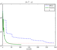
Fig. 1: Image deblurring with wavelets: Evolution of the quadratic constraint $\|{\bf AWx}-{\bf y}\|_{2}$ over time for $9\times 9$ uniform blur, $\sigma=0.56$

In the MRI reconstruction experiment, ${\bf M}$ models 22 radial observations of the DFT and $\phi$ is the TV norm [5]. Since SPGL1 can be used only for $\phi({\bf x})=\|{\bf x}\|_{1}$, we compare C-SALSA with the code available in $\ell_{1}$-magic. Table 3 compares the 2 algorithms, in terms of computation time and the final MSE obtained.

Table 3: MRI reconstruction - Comparison of computation speed

Algorithm	CPU time (seconds)	MSE
$\ell_{1}$-magic	710.997	0.000117224
C-SALSA	18.6875	6.79023e-007

5 Conclusions

We have proposed a fast algorithm for solving constrained convex optimization problems usually known as basis pursuit denoising. Our algorithm is based on variable splitting and exploits augmented Lagrangian tools. Preliminary experiments with $\ell_{1}$ and TV regularization show that the new algorithm outperforms existing methods in terms of computation time, by a considerable factor. Ongoing work includes a more thorough experimental evaluation of C-SALSA.

References

- [1] A. Beck and M. Teboulle. “A fast iterative shrinkage-thresholding algorithm for linear inverse problems”, SIAM Jour. on Imaging Sciences, vol. 2, pp. 183–202, 2009.
- [2] J. Bioucas-Dias and M. Figueiredo. “A new TwIST: two-step iterative shrinkage/thresholding algorithms for image restoration”, IEEE Trans. on Image Processing, vol. 16, no. 12, pp. 2992-3004, 2007.
- [3] J. Bioucas-Dias and M. Figueiredo. “An iterative algorithm for linear inverse problems with compound regularizers”, IEEE Int. Conf. on Image Proc. - ICIP’2008, San Diego, CA, USA, 2008.
- [4] J.-F. Cai, S. Osher, and Z. Shen. “Split Bregman methods and frame based image restoration,” SIAM Jour. Multisc. Model. Simul., 2009.
- [5] E. Candès, J. Romberg and T. Tao. “Stable signal recovery from incomplete and inaccurate information,” Communications on Pure and Applied Mathematics, vol. 59, pp. 1207–1233, 2005.
- [6] A. Chambolle. “An algorithm for total variation minimization and applications,” J. Math. Imaging Vis., vol. 20, no. 1-2, pp. 89–97, 2004.
- [7] A. Chambolle and P.-L. Lions. “ Image recovery via total variation minimization and related problems,” Numerische Mathematik, vol. 76, pp. 167–188, 1997.
- [8] S. Chen, D. Donoho, and M. Saunders. “Atomic decomposition by basis pursuit,” SIAM Jour. Scientific Comput., vol. 20, pp. 33–61, 1998.
- [9] P. Combettes and V. Wajs. “Signal recovery by proximal forward-backward splitting,” SIAM Jour. on Multiscale Modeling & Simulation, vol. 4, pp. 1168–1200, 2005.
- [10] D. Donoho. “Compressed sensing,” IEEE Trans. on Inform. Theory, vol. 52, pp. 1289–1306, 2006.
- [11] J. Eckstein and D. Bertsekas. “On the Douglas Rachford splitting method and the proximal point algorithm for maximal monotone operators”, Mathematical Programming, vol. 5, pp. 293 -318, 1992.
- [12] M. Figueiredo, J. Bioucas-Dias, “Deconvolution of Poissonian images using alternating direction optimization”, in preparation, 2009.
- [13] M. Figueiredo, J. Bioucas-Dias, and M. Afonso. “Fast frame-based image deconvolution using variable splitting and constrained optimization”, IEEE Work. on Stat. Sig. Proc. – SSP’2009, Cardiff, UK, 2009.
- [14] M. Figueiredo and R. Nowak. “An EM algorithm for wavelet-based image restoration.” IEEE Trans. Im. Proc., vol. 12, pp. 906–916, 2003.
- [15] M. Figueiredo, R. Nowak, S. Wright. “Gradient projection for sparse reconstruction,” IEEE J. Sel. Top. Sig. Proc., vol. 1, pp. 586–598, 2007.
- [16] T. Goldstein and S. Osher. “The split Bregman algorithm for regularized problems”, Technical Report 08-29, Computational and Applied Mathematics, UCLA, 2008.
- [17] M. Hestenes, “Multiplier and gradient methods”, Jour. of Optim. Theory and Appl.s, vol. 4, pp. 303–320, 1969.
- [18] S. Kim, K. Koh, M. Lustig, S. Boyd, and D. Gorinvesky. “ An interior-point method for large-scale -regularized least squares,” IEEE Jour. Selected Topics Sig. Proc., vol. 1, pp. 606–617, 2007.
- [19] M. Lustig, D. Donoho, and J. Pauly. “Sparse MRI: the application of compressed sensing for rapid MR imaging,” Magnetic Resonance in Medicine, vol. 58, pp. 1182–1195, 2007.
- [20] F. Malgouyres. “Minimizing the total variation under a general convex constraint for image restoration”, IEEE Trans. on Image Processing, vol. 11, pp. 1450–1456, 2002.
- [21] S. Mallat. A Wavelet Tour of Signal Processing, Academic Press, 2008.
- [22] J. Nocedal, S. J. Wright. Numerical Optimization, Springer, 2006.
- [23] S. Osher, L. Rudin, and E. Fatemi. “Nonlinear total variation based noise removal algorithms,” Physica D., vol. 60, pp. 259–268, 1992.
- [24] M. Powell, “A Method for nonlinear constraints in minimization problems”, in Optimization, R. Fletcher, (editor), Academic Press, pp. 283–298, New York, 1969.
- [25] S. Setzer. “Split Bregman algorithm, Douglas-Rachford splitting, and frame shrinkage”, 2nd Intern. Conf. on Scale Space Methods and Variational Methods in Computer Vision, Springer, 2009.
- [26] E. van den Berg and M. P. Friedlander. “Probing the Pareto frontier for basis pursuit solutions”, SIAM J. Sci. Comp., vol. 31, pp. 890–912, 2008.
- [27] Y. Wang, J. Yang, W. Yin, and Y. Zhang. “A new alternating minimization algorithm for total variation image reconstruction”, SIAM Jour. on Imaging Sciences, vol. 1, pp. 248–272, 2008.
- [28] S. Wright, R. Nowak, M. Figueiredo. “Sparse reconstruction by separable approximation , IEEE Tr. Sig. Proc., vol. 57, pp. 2479–2493, 2009.
- [29] W. Yin, S. Osher, D. Goldfarb, and J. Darbon. “Bregman iterative algorithms for minimization with applications to compressed sensing”, SIAM Jour. Imaging Science, vol. 1, pp. 143–168, 2008.