Buoyant bubbles in intracluster gas: effects of magnetic fields and anisotropic viscosity

Abstract

Recent observations by Chandra and XMM-Newton indicate there are complex structures at the cores of galaxy clusters, such as cavities and filaments. One plausible model for the formation of such structures is the interaction of radio jets with the intracluster medium (ICM). To investigate this idea, we use three-dimensional magnetohydrodynamic simulations including anisotropic (Braginskii) viscosity to study the effect of magnetic fields on the evolution and morphology of buoyant bubbles in the ICM. We investigate a range of different initial magnetic field geometries and strengths, and study the resulting x-ray surface brightness distribution for comparison to observed clusters. Magnetic tension forces and viscous transport along field lines tend to suppress instabilities parallel, but not perpendicular, to field lines. Thus, the evolution of the bubble depends strongly on the initial field geometry. We find toroidal field loops initially confined to the interior of the bubble are best able reproduce the observed cavity structures.

1 INTRODUCTION

In recent years, $Chandra$ observations of galaxy clusters have revealed complex structures such as cavities and filaments in the x-ray surface brightness distribution. The most prominent examples include Perseus (Fabian et al. 2000), Cygnus A (Carilli et al. 1994), Virgo-A (Young et al. 2002) and Hydra A (McNamara et al. 2000); a systematic study of 16 clusters is given by Birzan et al. (2004), and an extensive survey of 64 X-ray cavities in clusters, groups and elliptical galaxies is given by Diehl et al. 2008. Typically x-ray cavities are located at about 20 kpc (projected) from the cluster center, and have a radius of about 10 kpc. Interestingly, most of these systems harbor central galaxies with radio luminosities between $2\times 10^{38}$ and $7\times 10^{44}$ ergs s^-1. Moreover, $Chandra$ observations confirm that these clusters have an inwardly decreasing temperature profile, and therefore are so-called “cool core” clusters (Birzan et al. 2004).

One interpretation of the observations is that such structures are formed by the interaction of radio jets produced by a supermassive black hole (SMBH) in the central radio galaxy with the intracluster plasma. Such interaction will produced shocked jet material that is highly over-pressurized with respect to the ambient intracluster medium (ICM). As it expands to achieve pressure equilibrium, it will form a low density, high entropy cavity – that is a “bubble”. In the density stratified ICM, the bubble will be buoyant, and as it rises it evolves into the observed cavity-like structures. The feedback of radio jets on the ICM through the dynamics of pressure-inflated bubbles might be an important source of heating of the x-ray emitting plasma (Ruszkowski et al.2004; Fabian et al. 2005), and contribute to the prevention of the cooling catastrophe (Fabian 1994).

In order for this interpretation to be correct, rising bubbles in the ICM must remain coherent, and avoid being shredded by Rayleigh-Taylor instability (RTI), Richtmyer-Meshkov instability (RMI) and Kelvin-Helmholtz instability (KHI). A variety of authors have used numerical simulations to study the hydrodynamics of buoyant bubbles in two-dimensions (e.g., Bruggen & Kaiser 2001, 2002; Churazov et al. 2001; Bruggen 2003; Reynolds et al. 2002; Sternberg et al. 2007), and three-dimensions (e.g., Basson & Alexander 2003; Quilis et al. 2001; Omma et al. 2004; Gardini 2007; Pavlovski et al. 2008). Pizzolato & Soker (2006) have shown that in the early evolution, when the AGN jet is still inflating the bubble, it is stable to RTI, and Sternberg & Soker (2009a) studied the inflation of the bubbles by highly subrelativistic massive jets, and gave an example on a galaxy cluster (Sternberg & Soker, 2009b), while Fabian et al. (2005) have shown that the heating and cooling rates associated with weak shocks, viscosity and thermal conduction vary with temperature and radius in the ICM. Other recent three-dimensional hydrodynamic simulations include Bruggen et al. (2009) and Scannapieco & Bruggen (2008). A general result of all such studies is that purely inviscid hydrodynamical evolution generally can not produce the observed morphology of the cavities, nor reproduce the heating required to explain the observed temperature profile in the clusters. This suggests that additional physics is important to the dynamics, (Gardini 2007; Reynolds et al. 2005; Diehl et al. 2008): possible candidates include turbulent motions in the ICM, magnetic fields, viscosity and thermal conduction.

Since the hot gas in clusters of galaxies is likely magnetized (Carilli & Taylor 2002; Taylor et al. 2002), magnetohydrodynamic (MHD) effects could be important for the evolution of buoyant bubbles. Bruggen & Kaiser (2001) studied rising bubbles in two-dimensional MHD in spherical geometry to investigate the effect of magnetic fields on the RTI and KHI. A larger parameter survey, including various field geometries and strengths, and various profiles for the atmosphere, was presented by Robinson et al. (2004) for a two-dimensional planar geometry. Jones & De Young (2005) extended this work using spatially varying fields and internal fields generated self-consistently as the bubble is inflated. More recently, O’Neill et al. (2009) further extended the work of Jones & De Young (2005) to three-dimensional MHD simulations. Nakamura et al. (2006, 2007) studied the origin of magnetized bubbles. In their three-dimensional MHD simulations the SMBH injects poloidal and toroidal magnetic field into space and inflates the bubbles. Other three-dimensional MHD simulations include Ruszkowski et al. (2007), which focus on fossil bubbles in the presence of tangled magnetic fields; Liu et al. (2008), which presented long-term simulations of magnetized bubbles, and Dursi $ Pfrommer (2008), showing bubbles may develop a dynamically important magnetic sheath around themselves, which can suppresses instabilities at the surface of the bubbles. All of these authors confirm that a strong magnetic field parallel to the surface of the bubble can stabilize both KHI and RTI during the evolution, as expected from the linear stability analysis (Chandrasekhar 1961; Shore 1992). Fully three-dimensional studies are important for this problem, however, because magnetic fields only suppress RTI for modes parallel to the field; they have no effect on interchange modes perpendicular to the field. Thus, fully three dimensional studies of the magnetic RTI (Stone & Gardiner 2007a; b) have shown rapid growth of unstable fingers even in the case of strong fields.

Viscous effects may also be important to the dynamics (Fabian et al. 2003), since the Reynolds number in the intracluster gas is so low. Using the standard Spitzer (1962) estimate for the coefficient of viscosity leads to an estimate of the Reynolds number of

$$Re=62\left(\frac{U}{390\ \rm{km\ s}^{-1}}\right)\left(\frac{L}{20\ \rm{kpc}}\right)\left(\frac{\rm{kT}}{5\ \rm{keV}}\right)^{-2.5}\left(\frac{n}{0.03\ \rm{cm}^{-3}}\right)\left(\frac{\ln\Lambda}{30}\right)$$ (1)

where $U$ is the typical velocity of motions (scaled to one half the adiabatic sound speed for hydrogenic plasma at $kT=5$ keV), and $L$ is a typical length scale for the bubble (Reynolds et al. 2005). Ruszkowski et al. (2004) studied viscous dissipation of the gas motions and sound waves generated by buoyant bubbles, and the implications for heating of the ICM. Reynolds et al. (2005) studied the effect of viscosity on the morphology and evolution of bubbles, including comparisons between the synthetic x-ray surface brightness of bubbles in their hydrodynamic simulations with observations. These authors pointed out that a coefficient of viscosity that is only 25 percent of the Spitzer value can quench the development of instabilities and maintaining the integrity of the bubble.

However, in a weakly-collisional plasma such as the ICM, microscopic transport processes such as viscosity and thermal conduction will be anisotropic when the collision mean free path of ions or electrons is much larger than their Larmor radius. For example, momentum transport by viscosity (which is mediated primarily by ion-ion collisions) will be anisotropic when

$$\epsilon\equiv(\omega_{c,i}\tau_{c,i})^{-1}\ll 1$$ (2)

where $\omega_{c,i}$ is the ion cyclotron frequency and $\tau_{c,i}$ is the ion-ion mean collision time. For a hydrogenic plasma, this condition can be written as

$$\omega_{c,i}\tau_{c,i}=(\frac{1.09\times 10^{5}}{n})\frac{T_{4}^{1.5}B_{\mu G}}{ln\Lambda}$$ (3)

where $n$ is the proton density in cm^-3, $T_{4}$ is the kinetic temperature in units of $10^{4}$K, $B_{\mu\mathrm{G}}$ is the magnetic field in microgauss. In the ICM, typical temperatures are $T\sim 10^{7}$ K and typical densities are $n\sim 10^{-3}-10^{-2}$ cm^-3 (Peterson & Fabian 2006). The magnetic field strength is roughly $B\sim 1-10$ $\mu$G at the center of a typical cluster, and 0.1-1 $\mu$G in the outer regions. For these values, clearly $\epsilon\ll 1$, and viscous transport will be anisotropic. In addition, we note that $\beta=(8\pi p)/(B^{2})$, the ratio of the gas to magnetic pressure, is large for the conditions in a typical cluster ( $\beta\approx 200-2000$ in the central regions) (Parrish et al. 2008), which is an indication that the magnetic field is dynamically unimportant. However, due to anisotropic transport effects, the existence of even a weak magnetic field will still dramatically influence the physical transport processes.

Recently, the effect of anisotropic transport processes in weakly collisional plasmas has been studied both theoretically (Balbus 2004; Islam & Balbus 2005; Lyutikov 2007, 2008) and numerically (Sharma et al. 2006; Parrish & Quataert 2008; Quataert 2008; Parrish et al. 2008,2009) in a number of astrophysical systems. In the context of clusters, Balbus (2000) has shown that anisotropic thermal conduction produces qualitatively new effects, such as modifying the convective stability criterion (the magnetothermal instability or MTI). Parrish & Stone (2005; 2007a; b) and Parrish et al. (2008) have studied the nonlinear saturation of the MTI, while Parrish et al. (2008) investigated the effect of the MTI on the evolution of the temperature profile in the ICM. Quataert (2008) pointed out that in the presence of a background heat flux, anisotropic thermal conduction will drive a new buoyancy instability (the heat flux buoyancy instability, or HBI) when the temperature decreases in the direction of gravity, and Parrish & Quataert (2008), Sharma et al. (2009), Parrish et al. (2009) and Bogdanovic et al. (2009) have studied the HBI using three-dimensional MHD simulations. Lyutikov (2007, 2008) has emphasized the importance of anisotropic transport in the ICM, arguing that it determines the dissipative properties, the stability of embedded structures, and the transition to turbulence in the ICM. Thus, simulations of the dynamics of the ICM using isotropic versus anisotropic transport (viscosity or thermal conduction) can produce quite different results.

The goal of this work is to study the effect of anisotropic viscosity and magnetic fields on the dynamics of buoyant bubbles in the ICM. Although other physical processes, such as turbulence and cosmic rays generated by merging substructures, or thermal conduction, could be important for interpreting the observations of structures in the ICM, we will not include such processes here. Our goal is simply to investigate the role of magnetic fields and anisotropic viscosity on the RTI and KHI in rising bubbles, using different field strengths and directions, and to compare the morphology of bubbles computed with realistic values of the parameters with the observations. Our study can be considered as an extension of previous MHD simulations that did not include viscosity, or previous viscous simulations that did not include MHD.

This paper is organized as follows. In §2 we review the basic physics in the simulations, and we describe the numerical methods used in this work. In §3 we present results from our simulations, including the evolution of the density profile and simulated x-ray images. In §4 we discuss the implications of our results for models of AGN feedback and heating, and in §5 we present our conclusions.

2 Method

We solve the equations of MHD, which can be written in conservative form as

$$\frac{\partial\rho}{\partial t}+{\bf\nabla\cdot}(\rho{\bf v})=0,\\$$ (4)

$$\frac{\partial(\rho{\bf v})}{\partial t}+{\bf\nabla\cdot}\left(\rho{\bf vv}-\frac{\bf BB}{4\pi}+P+\frac{\bf B^{2}}{8\pi}-\bar{\bf\sigma}\right)=-\rho{\bf\nabla}\Phi,\\$$ (5)

$$\frac{\partial(\rho E)}{\partial t}+{\bf\nabla\cdot}\left(\rho E\bf v+\left[p+\frac{\bf B^{2}}{8\pi}\right]\bf v-\frac{(\bf v\cdot\bf B)\bf B}{4\pi}-\bf v\cdot\bar{\bf\sigma}\right)=\rho{\bf v}\cdot{\bf\nabla}\Phi,\\$$ (6)

$$\frac{\partial{\bf B}}{\partial t}-{\bf\nabla}\times\left({\bf v}\times{\bf B}\right)=0,$$ (7)

where $\Phi$ is a fixed gravitational potential due to the dark matter, $E$ is the total energy (sum of internal, kinetic and magnetic energies, but excluding the gravitational potential energy), and ${\bf\sigma}$ is the viscous stress tensor. The other symbols have their usual meaning. We have written these equations in units such that the magnetic permeability $\mu_{B}=1$. In a magnetized plasma, the anisotropic viscous stress tensor can be written as (Balbus 2004),

$$\sigma_{ij}=\mu\left(\frac{B_{m}B_{k}}{\bf B^{2}}\partial_{k}v_{m}-\frac{\nabla\cdot\bf v}{3}\right)\left(\frac{B_{i}B_{j}}{\bf B^{2}}-\delta_{ij}\right)$$ (8)

where summation over repeated indices is implied. We fix the coefficient of viscosity $\mu$ to be a constant parameter for all the simulations presented here.

The effects of the dark matter on the dynamics is strictly through gravitational forces represented by a fixed potential. Following Reynolds et al. (2005), we assume the dark matter potential is given by

$$\Phi=\frac{0.75}{\gamma}\log(1+r^{2})$$ (9)

We assume the ICM forms an isothermal hydrostatic equilibrium in this potential, so that $\rho(r)=\rho_{0}[1+(\frac{r}{r_{0}})^{2}]^{-0.75}$ and $P=c_{s}^{2}\rho$, where we choose units of mass, length, and time such that $\rho_{0}=1$, $r_{0}=1$, and $c_{s}=1$.

At the start of the calculation, we introduce a bubble into this atmosphere as a spherical region offset from the center of the dark matter potential a distance $R=0.3$, with density $\rho_{b}=0.01(1+\delta)$ and radius $r_{b}=0.25$. We introduce perturbations to the density in the bubble through $\delta$, a random number chosen independently for each computational cell contained within the bubble, with $|\delta|\leq 0.005$. We find such perturbations are necessary to break the symmetry of the resulting evolution, otherwise our numerical scheme will preserve such symmetries exactly. Initially the bubble is in pressure equilibrium with its surroundings. The evolution of the bubble is computed using an adiabatic equation of state with $\gamma=5/3$. Note we do not attempt to model the formation and inflation of the bubble via the interaction of a radio jet with the ICM. Instead, and following previous authors, we simply introduce a buoyant bubble into a hydrostatic atmosphere and follow the resulting dynamics.

Our calculations use Athena (Stone et al. 2008), a recently developed Godunov scheme for astrophysical MHD. The mathematical foundations of the algorithms are documented in Gardiner & Stone (2005; 2008). The directionally unsplit CTU (corner transport upwind) integration scheme, combined with the Roe Riemann solver, are used throughout. Extensive tests of the algorithms are presented in Stone et al. (2008). The gravitational source terms due to the dark matter potential are added to the interface reconstruction, transverse flux gradient corrections, and final corrector update in the CTU integration algorithm directly to preserve second order accuracy, and in a way that conserves the total energy (including gravitational potential energy) exactly. Anisotropic viscosity is added through operator splitting. In order to conserve total momentum exactly, we difference the viscous fluxes at each cell interface, which requires that the components of ${\bf\sigma}$ be centered at the appropriate cell faces. We use TVD (total variation diminishing) slope limiting to construct the velocity differences when computing the stress, using a method that is exactly analogous to computing the heat fluxes with anisotropic conduction (Sharma & Hammett 2007). This step is crucial to preventing unphysical momentum fluxes. The details of our algorithm are presented in the Appendix in Stone & Balbus (2009).

Our simulations use a Cartesian grid that spans a domain $-1\leq x\leq 1$, $0\leq y\leq 3$, and $-1\leq z\leq 1$. The origin of the dark matter potential $r=0$ is located at $(x,y,z)=(0,0,0)$, and the center of the bubble is located initially along the $y-$axis at $(x,y,z)=(0,0.3,0)$. The bubble rises in the $y-$direction, hereafter we refer to this direction as the “vertical”. Our typical numerical resolution is $256\times 384\times 256$, although we present a convergence study in which we both double and halve this resolution in each direction. We use reflecting boundary condition at $y=0$ and outflow boundary conditions everywhere else. At outflow boundaries, we project all quantities with zero slope, except the pressure, which we compute from integrating the equation of hydrostatic equilibrium into the ghost zones using the pressure in the last active cell as an initial condition. We find this step maintains hydrostatic equilibrium near the boundaries of the domain quite well. Even though we allow material to flow freely through the boundaries, we find that by the end of each simulation the mass lost is less than $5\times 10^{-4}$ of the initial value. Due to our outflowing boundary conditions, the total energy of the gas (including the gravitational potential energy) in our simulations is not conserved, although we find that the fractional change in the total energy in the domain is small, less than $10^{-3}$. Lack of strict conservation of energy complicates the measurement of the work done on the gas by rising bubbles, we examine this issue in more detail in §4.2.

We study three different initial magnetic field configurations, including (1) a uniform horizontal field ${\bf B}=(B_{0},0,0)$, (2) a uniform vertical field ${\bf B}=(0,B_{0},0)$, and (3) a uniform toroidal field of strength $B_{0}$ located only inside the bubble. In the first two cases the field is located throughout the domain (within both the bubble and the atmosphere). In the toroidal field case, the field lines form concentric loops inside the bubble, and there is no field outside the bubble. In this case the field is initialized from a vector potential via ${\bf B}=\nabla\times\bf A$, where the components of ${\bf A}$ are defined at cell edges, with the only non-zero component

$$A_{y}=B_{0}(\sqrt{0.25^{2}-(y-0.3)^{2}}-\sqrt{x^{2}+z^{2}}),$$ (10)

This procedure guarantees the initial field satisfies the divergence-free constraint exactly. For each field geometry, we study two different field strengths: a weak field given by $\beta=2\rho_{0}c_{s}^{2}/B_{0}=1.2\times 10^{6}$, and a strong field given by $\beta=480$.

We can relate the units used in the simulations to quantities in real clusters by adopting fiducial values for length, mass and time. For example, if we fix the unit of length used in the code to 20 kpc, the unit of mass to be given by the density $\rho_{0}=1$ being equivalent to a proton number density of 0.03 cm^-3, and the unit of time to be fixed by the adiabatic sound speed $c_{s}=1$ being equivalent to 800 km s^-1, then our simulation domain spans a region $40\times 40\times 60$ kpc, our typical numerical resolution is about 0.16 kpc, and the sound crossing time is about 25 Myr. Furthermore, the weak field case corresponds to a magnetic field strength of 0.05 - 0.10 $\mu$G, while the strong field case about 1 - 5 $\mu$G.

3 Results

We present the results from 11 different simulations (although we have run many more to test our methods and survey parameters). For those simulations that include viscosity, we fix the coefficient of viscosity $\mu$ to give a Reynolds number $Re=c_{s}L\rho_{0}/2\mu=50$ (using $c_{s}/2$ as the characteristic velocity in the problem), where in the code units $c_{s}=L=\rho=1$. We report results from two purely hydrodynamic simulations performed as control experiments for comparison to the MHD cases. One of these simulations is inviscid, and one has been run with an isotropic Navier-Stokes viscosity with a Reynolds number of 50. The remaining 9 simulations correspond to each of the three magnetic field geometries (horizontal, vertical, and toroidal) run with both a weak and strong field with anisotropic viscosity, and a strong field with no viscosity. We have confirmed that simulations run with a weak field and no viscosity are nearly identical to the inviscid hydrodynamic case, and thus such models will not be discussed further. We have run the strong field cases both with and without viscosity in order to isolate the effects of the magnetic field (MHD) from the effects of the anisotropic viscosity. Table 1 summarizes the properties of all the simulations presented here.

Table 1: Property of the simulations presented in this paper

Label	Re	$\beta$	Field direction
$H1$	-	-	-
$H2$	50	-	-
$X1$	50	$1.2\times 10^{6}$	horizontal
$X2$	-	480	horizontal
$X3$	50	480	horizontal
$Y1$	50	$1.2\times 10^{6}$	vertical
$Y2$	-	480	vertical
$Y3$	50	480	vertical
$T1$	50	$1.2\times 10^{6}$	toroidal
$T2$	-	480	toroidal
$T3$	50	480	toroidal

3.1 Convergence test

It is important to confirm that our standard numerical resolution, $256\times 384\times 256$, is sufficient to resolve the flow. Since we are studying a relatively low Reynolds number ($Re=50$), we expect that achieving numerical convergence will not be difficult. To study numerical convergence we have run model H2 at three different resolutions: $128\times 192\times 128$ (low resolution), $256\times 384\times 256$ (standard resolution), and $512\times 768\times 512$ (high resolution). Figure 1 shows the convergence of $\langle v_{y}\rangle$, the vertical component of the velocity averaged over a spherical shell as a function of the radius $r=\sqrt{x^{2}+y^{2}+z^{2}}$ of that shell, at $t=8$ for each of these three resolutions. We expect the vertical velocity to be a good indicator of convergence since it measures the buoyant motion of the bubble. Note the overall radial profile of the vertical velocity is very close at each resolution. The difference between the highest and our fiducial resolution simulation is less than $10\%$ at every radius, and this difference is everywhere smaller than that between the fiducial and the lowest resolution simulations, which is the hallmark of convergence.

Figure 1 also shows the time evolution of the volume averaged kinetic energy $E_{k}=\int_{V}\rho v^{2}/2dV$ for each different resolution. Initially $E_{k}=0$, but as the bubble rises the kinetic energy quickly evolves. The largest difference in $E_{k}$ between the low and fiducial resolution runs is reached at $t=8$, and is about $15\%$, while the difference between the standard and high resolution cases is much smaller, about $5\%$ at $t=8$. Once again, the decrease in this difference with numerical resolution is an indication of convergence.

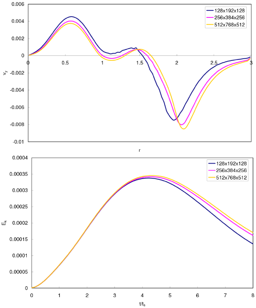
Figure 1: (Top.) Radial profile of the angle-averaged vertical velocity at $t=8$ in run H2 computed with three different numerical resolutions. (Bottom.) Volume averaged kinetic energy as a function of time for run H2 at three different resolutions.

Finally, Figure 2 show the density of the bubble in a slice through the midplane ($z=0$) in run H2 at $t=8$ using these three numerical resolutions, in order to compare the morphology of the bubble as an indication of convergence. Note the bubble in the standard and high resolution simulations is nearly identical, while the differences between the standard and low resolution simulations are also small. Based on these results, we have confidence that the standard resolution used in this study is sufficient.

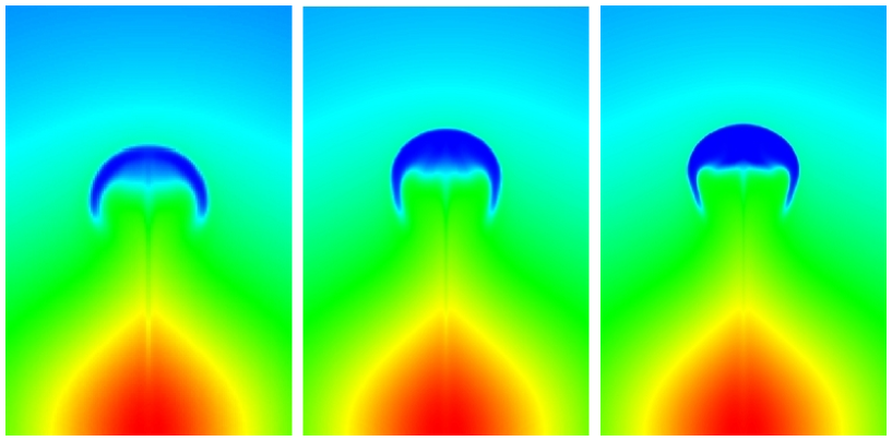
Figure 2: Slice of the density through the midplane ($z=0$) in run H2 at $t=8$ for three different numerical resolutions. From left to right: $128\times 192\times 128$, $256\times 384\times 256$, and $512\times 768\times 512$. There is very little difference in the structure of the bubble between the latter two. A linear color scale from $\rho=0$ to $\rho=1$ is used.

3.2 Hydrodynamic Models

To confirm that we reproduce previous inviscid and viscous hydrodynamic simulations, and to provide a benchmark for comparison of the MHD models presented below, we first discuss runs H1 (inviscid) and H2 (isotropic viscosity with $Re=50$). Figure 3 shows slices of the density at the mid-plane ($z=0$) for these runs at three different times. The most striking feature in the plots is the emergence of RTI at the top of the bubble, and KHI along the edges, in run H1 (top row of plots). As a results of these instabilities, the bubble interface is highly distorted, material from the ICM can penetrate the bubble, and the bubble is subsequently shredded and diffused into the ICM. As shown by Reynolds et al. (2005), an isotropic Navier-Stokes viscosity suppresses these instabilities, and mixing. The bottom row of plots shows run H2, which has a Reynolds number of 50. Clearly the evolution of the bubble is dramatically altered. The viscosity quenches the instabilities, and the bubble remains intact throughout the evolution.

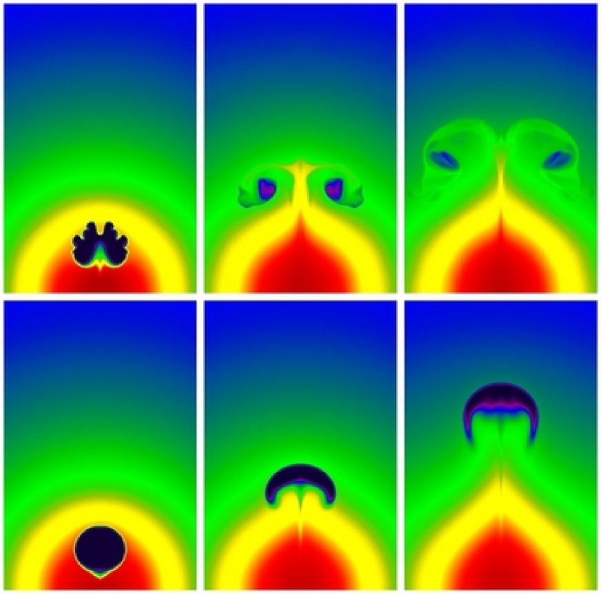
Figure 3: Slices of the density at the midplane ($z=0$) at $t=1$ (left column), $t=4$ (middle column) and $t=8$ (right column) for run H1 (top row) and H2 (bottom row). A linear color scale from $\rho=0$ to $\rho=1$ is used.

Reynolds et al. (2005) also presented synthetic x-ray images of their simulations, computed assuming an x-ray emissivity proportional to $\rho^{2}T^{0.5}$ which is then integrated along the line of sight. These authors showed that the inviscid model (equivalent to H1) cannot reproduce observed features such as cavities, since the bubble is shredded by instabilities. On the other hand, the morphology of the bubble in the viscous case (equivalent to H2) shows good agreement with observations. We have computed synthetic images of our simulations, and are able to reproduce these results (see §4.1).

3.3 Uniform horizontal field

We now turn to models with a uniform horizontal magnetic field throughout the domain (including the bubble) initially. Figure 4 shows slices of the density in runs X1 (weak horizontal field and anisotropic viscosity), X2 (strong horizontal field and no viscosity), and X3 (strong horizontal field and anisotropic viscosity), at three different times, $t=1,4$ and 8. Since the horizontal field breaks axisymmetry, slices along both the planes $x=0$ and $z=0$ are shown using a perspective plot. Initially, the field is entirely in the $x-$direction, that is perpendicular to the slice at $x=0$, and in the plane of the slice at $z=0$.

The top row of images shows the evolution of the density in model X1. It is useful to compare this evolution directly to run H2 shown in the bottom row in figure 3. Unlike the hydrodynamic case with isotropic viscosity, the images show that in a weak magnetic field with anisotropic viscosity, the bubble is shredded by RTI and KHI, although in a complex manner. In the $y-z$ plane, perpendicular to the direction of the magnetic field, the bubble splits into two halves, and there are clear KH rolls that develop in this plane. In the $x-y$ plane, parallel to the field, the bubble surface shows less instability and distortions. Viscosity along the field lines in this plane suppresses instability.

The second row of Figure 4 shows the evolution of the density in model X2. Interesting, although there is no viscosity in this calculation, the evolution is similar to model X1. Once again, the bubble is shredded by KHI and RTI, splitting apart with strong mixing in the $y-z$ plane, and remaining more coherent in the $x-y$ plane. This evolution is a clear indication of the anisotropic suppression of RTI in strong magnetic fields (Stone & Gardiner 2007a; b). Perpendicular to the field, interchange modes grow rapidly, splitting the bubble and causing mixing, while parallel to the field magnetic tension suppresses the RTI and the bubble remains more intact. In comparison to run X1, there is more diffusion and mixing, and smaller scale structures develop in run X2.

Finally, the bottom row in Figure 4 shows the evolution of the density in model X3. Once again, the overall evolution is similar to runs X1 and X2: the bubble is split into two halves, with strong mixing and small scale KHI in the $y-z$ plane, and less instability and mixing in the $x-y$ plane. While in run X1 (top row) the bubble remained intact until the final time, in run X3 instabilities almost entirely destroy the bubble, with the hot plasma in the bubble completely mixed with its surrounding colder gas. The similar evolution observed in all three of these runs is an indication that uniform horizontal fields play a similar role to anisotropic viscosity along weak fields of the same geometry in the evolution of rising bubbles.

For the strong field runs X2 and X3, the final magnetic field geometry largely maintains its initial structure at the final time, while in the weak field run X1 the final field structure is highly tangled. The ratio of the magnetic energies in the vertical and horizontal components of the field $B_{y}^{2}/B_{x}^{2}$ is 0.76 for run X1, 0.32 for X2 and 0.23 for X3. Thus, the field is still mostly horizontal at the end of runs X2 and X2, while it is nearly isotropic in run X1.

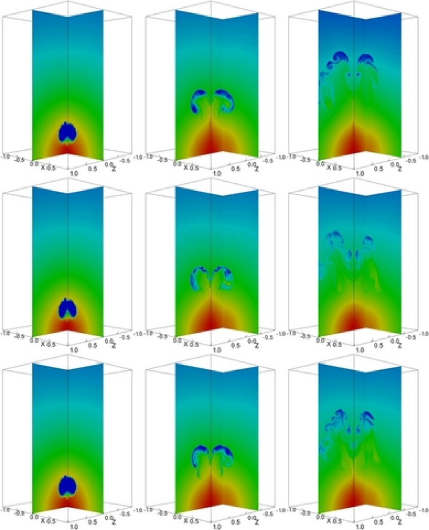
Figure 4: Slices of the density in the $y-z$ plane (left half of each plot) and $x-y$ plane (right half of each plot) at $t=1$ (left column), $t=4$ (middle column) and $t=8$ (right column) for runs beginning with an initially horizontal magnetic field. The top row shows the evolution of run X1, the middle row X2, and the bottom row X3. A linear color scale from $\rho=0$ to $\rho=1$ is used. (Note the $x-y$ plane plot at $t=1$ is at $z=0$, while at $t=4$ and $t=8$ it is at $z=-0.4$)

3.4 Uniform vertical field

Figure 5 shows slices of the density at three different times ($t=1,4$, and 8) in the $x-y$ plane in runs Y1 (weak vertical field and anisotropic viscosity), Y2 (strong vertical field and no viscosity), and Y3 (strong vertical field and anisotropic viscosity). Since the evolution is axisymmetric with vertical fields apart from grid effects (with a Cartesian grid, the bubble actually shows quadripole symmetry at late times), only one slice in any vertical plane is sufficient to show the structure of the bubble.

The top row of images shows the evolution of run Y1. In these runs, the growth of secondary KHI produces vortex rolls that wind up the vertical field. In turn, the field tries to resist the winding motion. In the weak field case shown in run Y1, the KHI largely overwhelms the magnetic tension, and the bubble is shredded and diffuses significantly into the ambient medium by the end of the simulations, with little hot plasma still being inside the bubble. Compared to the purely hydrodynamic model H2, we see that anisotropic viscosity has altered the overall evolution; the bubble splits into a ring instead of remaining coherent, and this ring spreads laterally away from the axis of symmetry. However, in contrast to the hydrodynamic case, anisotropic viscosity in run Y1 does not suppress the shredding or mixing of the bubble.

The middle row in Figure 5 shows the evolution in run Y2. As in run Y1, the bubble develops into a ring, with significant lateral spreading. The development of RTI is obvious at early times, (the first image at $t=1$). Large amplitude fingers are clearly visible; the largest finger at the center of the bubble ultimately results in splitting the bubble into a ring. Note the development of these fingers relies somewhat on the high degree of symmetry in the initial conditions. If the bubble were not initially axisymmetric, the resulting structure of the bubble would change. Once again, the similarities between runs Y1 and Y2 indicate that a strong field has similar effects on the dynamics of rising bubbles as an anisotropic viscosity.

The bottom row in Figure 5 shows the evolution in run Y3. The evolution is quite different in comparison to the previous two. Now, horizontal motions are strongly suppressed compared to vertical motions, and a large amount of material originally in the bubble remains concentrated within a small volume near the axis of symmetry at the end of the simulation. The initial spherical bubble evolves into a cone that roughly occupies a vertical column with transverse width equal to the original size of the bubble. The bubble does not remain a single coherent entity, however, but is split into many small columns by RTI fingers.

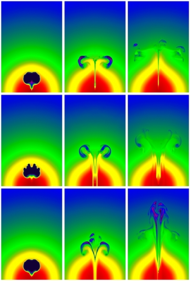
Figure 5: Slices of the density in the $x-y$ plane at $t=1$ (left column), $t=4$ (middle column) and $t=8$ (right column) for runs beginning with an initially vertical magnetic field. The top row shows the evolution of run Y1, the middle row Y2, and the bottom row Y3. A linear color scale from $\rho=0$ to $\rho=1$ is used.

For these vertical field runs, the magnetic field geometry does not change significantly with time, especially in the strong field with viscosity case. The ratio of magnetic energies in the horizontal and vertical components of the field $(B_{x}^{2}+B_{z}^{2})/B_{y}^{2}$ is 0.10 for model Y1, 0.07 for Y2 and 0.03 for Y3. This indicates for all three runs that only a small amount of magnetic energy is transformed from the vertical to the horizontal directions. The field lines are only weakly tangled, indicating the field roughly maintains its initial ordered configuration.

To investigate the evolution of very strong vertical fields, we ran several simulations with different values of $\beta\leqslant 1$. Interestingly, we found the bubble does not rise at all in this case. The upward movement of the bubble requires the ambient plasma above the bubble to move laterally and around the sides. With a very strong field, the magnetic tension is so strong it prevents any lateral movement of the fluid above the bubble, and the bubble is unable to rise. We note this result is quite different that reported by Robinson et al. (2004), who found rising bubbles even with $\beta=0.019$. We are uncertain as to the cause of this discrepancy, but speculate that it might reflect differences in the numerical algorithms.

3.5 Toroidal field confined to the bubble interior

Figure 6 shows slices of the density at three different times ($t=1,4$, and 8) in the $x-y$ plane in runs T1 (weak toroidal field just inside the bubble and anisotropic viscosity), T2 (strong toroidal field just inside the bubble and no viscosity), and T3 (strong toroidal field just inside the bubble and anisotropic viscosity). As in the vertical field case, since the bubble evolution is axisymmetric only one slice in a single vertical plane is sufficient to show the structure of the bubble (as before, the bubble actually has quadripole symmetry on our Cartesian grid).

The top row of images shows the evolution of run T1. As in the vertical field case run Y1, the bubble evolves into a ring at late times. However, unlike run Y1, this ring remains relatively coherent, and is not shredded by RTI and KHI. Since the magnetic field is everywhere parallel to the surface of the bubble, viscous transport along the field lines is able to suppress significant mixing with a toroidal field.

The middle row in Figure 6 shows the evolution in run T2. Once again due to the development of RTI fingers at early times, the bubble forms a ring (actually two rings, with one small and narrow ring formed above the main structure). However, hoop stresses associated with the strong field in this case keeps this ring coherent, and even at late time the ring is quite prominent and is not shredded by secondary KHI. Even at the end of the simulation $t=8$, the ring contains a significant amount of hot plasma.

The bottom row in Figure 6 shows the evolution in run T3. Again, as in the previous two toroidal field simulation, the bubble evolves into a ring. At the earliest time ($t=1$), the combination of viscosity and a strong field in run T3 suppresses the RTI in comparison to run T2 – there are fewer fingers in this case, and they are smaller in comparison to run T2. Hover, at late times ($t=8$), there is more small scale structure in the bubble in run T3 than T2, although the gross features of the ring are very similar in both cases. This demonstrates the complexity of the effects of anisotropic viscosity.

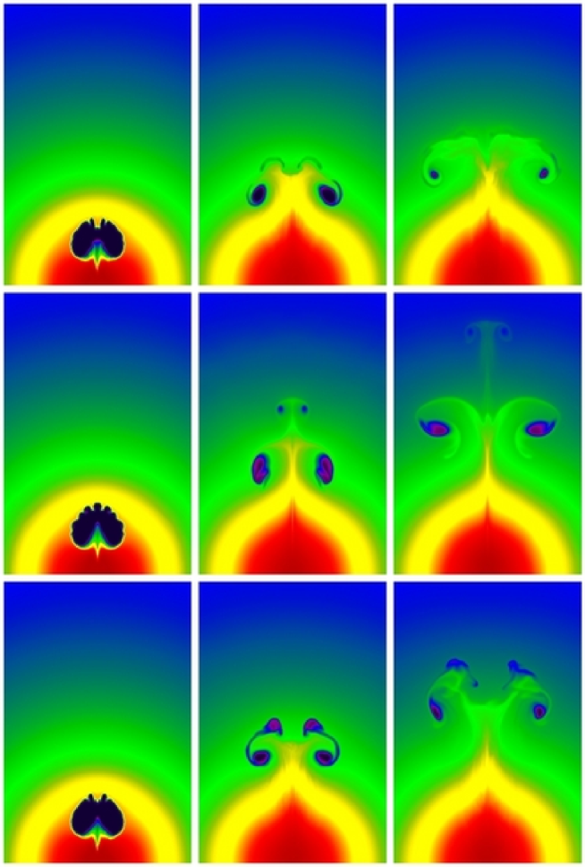
Figure 6: Slices of the density in the $x-y$ plane at $t=1$ (left column), $t=4$ (middle column) and $t=8$ (right column) for runs beginning with an initially toroidal magnetic field confined to the interior of the bubble. The top row shows the evolution of run T1, the middle row T2, and the bottom row T3. A linear color scale from $\rho=0$ to $\rho=1$ is used.

4 Discussion

4.1 Synthetic x-ray images

One of the primary goals of this project is to study whether bubble rising in a stratified atmosphere with realistic physics for the ICM (magnetic fields and anisotropic viscosity) can produce structures reminiscent of the cavities and filaments seen in the x-ray surface brightness distribution of observed systems (e.g. Birzan et al. 2004). To compute synthetic x-ray images of our simulations, we assume an x-ray emissivity proportional to $\rho^{2}T^{0.5}$, and integrate along the line of sight. As discussed in §3.2, synthetic x-ray images of our hydrodynamic simulations (both H1 and H2) look identical to those presented in figure 4 of Reynolds et al. (2005), and so we do not reproduce them here. An important conclusion of these authors is that inviscid evolution of the bubble shreds it into small scale features that do not reproduce the observations. We note that the X-ray surface brightness images generated from our simulations are idealized, and do not contain noise or background signal. Furthermore, the resolution of our synthetic images is the spatial resolution used in the code, which typically is much higher than the resolution in real observations. (For a computational domain of size $40\times 40\times 60$ kpc, our image resolution is 0.16 kpc. For typical clusters like Cygnus A, about 237 Mpc from us and Hydra A, about 240 Mpc form us, the image resolution on the Chandra ACIS chips will be 0.5 kpc; while for closer clusters like Perseus, about 72 Mpc from us, the resolution is comparable, about 0.17 kpc.) For these reasons, detailed comparison between our results and specific observations could be misleading, so that we will focus only on the general characteristics of the images.

Figure 7 shows simulated x-ray surface brightness images for runs X1, X2, and X3 at $t=4$, along two sightlines. As one might expect given the anisotropic structure of the bubbles evident in Figure 4, the morphology of the bubble in these images strongly depends in the sightline. When viewed perpendicular to the $x-y$ plane, all three cases produced coherent bubbles with a similar morphology: a bright cap with a darker cavity behind. This morphology is reminiscent of the structures of hydrodynamic bubbles with viscosity (e.g. run H2; see figure 4 in Reynolds et al. 2005), but shows more small scale structure in the region below the cap. On the other hand, when viewed perpendicular to the $y-z$ plane, the bubble is split into two crescent-shaped bright structures, with a dark lobe below each.

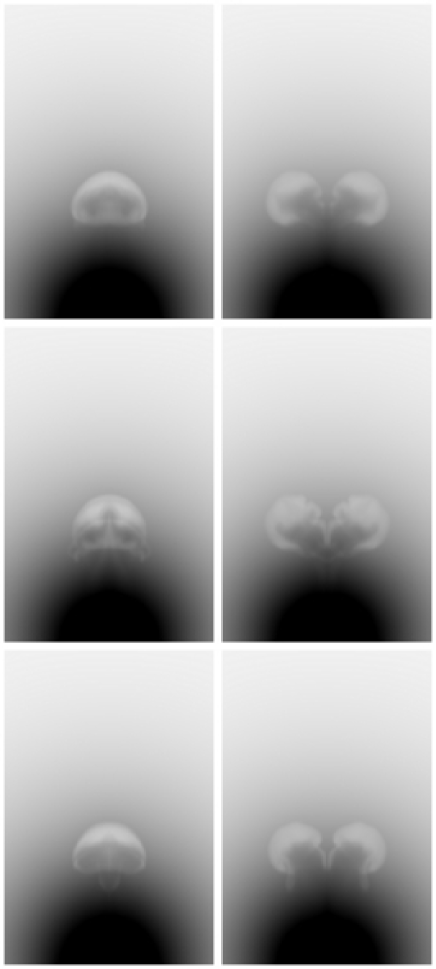
Figure 7: Synthetic x-ray surface brightness images of runs X1 (top row), X2 (middle row), and X3 (bottom row) at $t=4$. Images in the left column correspond to viewing the bubble along the $z-$axis, the right column corresponds to the view along the $x-$axis.

It is clear from inspection of Figure 5 that with vertical fields, the bubble is shredded by instabilities even with anisotropic viscosity. Thus, simulated x-ray images of the bubbles with vertical fields do not show cavities or filaments reminiscent of observations, and we do not show such images here.

In Figure 8, we show synthetic x-ray images of each of the three toroidal field simulations, at three different times. The ring structure of the bubble produced in all these cases is obvious. A toroidal field, either with or without viscosity, produces cavities in the x-ray surface brightness similar to observations, especially in runs T1 and T2 (top and middle rows of Figure 8). Although the structure formed here is ring-like instead of a uniform bubble, it is impossible to rule out this morphology given current observations. The image quality and resolution of current X-ray telescopes do not allow distinction between the two structures based on their two-dimensional surface brightness.

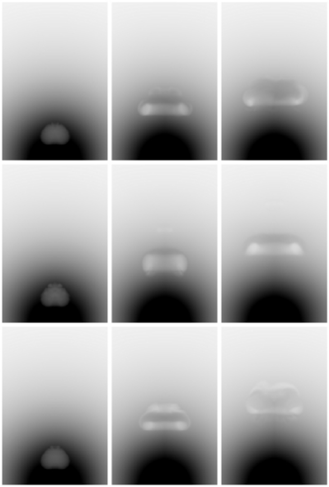
Figure 8: Synthetic x-ray surface brightness images for runs T1 (top row), T2 (middle row), and T3 (bottom row) at $t=1$ (left column), $t=4$ (middle column), and $t=8$ (left column).

We conclude that initially horizontal fields (when viewed perpendicular to the direction of the field), or toroidal magnetic fields confined to the interior of the bubble, produce “ghost cavity” structures reminiscent of x-ray images by Chandra and XMM-Newton. However, for vertical fields, such cavities cannot be reproduced. Both strong magnetic fields, or weak fields with anisotropic viscosity, are able to reproduce these features with the appropriate initial field geometry. The most realistic field geometry for bubbles inflated by AGN is likely a toroidal field confined to the interior of the bubble. Thus, the fact this geometry reproduces observations is reassuring.

4.2 Heating and AGN feedback

Another important goal of this study is to attempt to measure the heating rate of the ICM due to MHD processes associated with rising bubbles generated by AGN, using more realistic physics (magnetic fields and anisotropic viscosity). However, because of our use of open (outflow) boundary conditions in the simulations, total energy is not conserved, which can complicate such measurements. To investigate how much the total energy changes, compared to the changes in the internal energy, Figure 9 shows the fractional change in the volume averaged gravitational energy ($E_{G}=\int\rho\phi dV/V$), the volume averaged total energy $E_{t}$ (sum of the kinetic, internal, and gravitational energies) and the difference between the two $\delta E=E_{t}-E_{G}$, scaled by their initial values, as a function of time $t$ in run H1. The gravitational energy first decreases as the bubble rises due to buoyancy. This process releases potential energy which can be converted into other forms. The total energy $E_{t}$ increases a little with time, reaching a maximum at about $t=6$, at which point it is only $0.1\%$ larger than the initial value. This increase is due to work done on the system at the boundary. However, note that the change in total energy is less than the gravitational potential energy released by the rising bubble. Thus, any increase in the other forms of energy, including the internal energy of the ICM, will be dominated by the release of gravitational energy, and not the work done on the boundaries. Thus, tracking the changes in each form of energy in our simulations should give us a good estimate of the energy input due to the dynamics of the rising bubble.

Figure 9: Time evolution of the volume averaged gravitational energy $E_{G}$, total energy $E_{T}$, and the gas energy, which is the difference between the two $\delta E=E_{t}-E_{G}$, for run H1.

Figure 10 shows the fractional change of volume averaged internal energy $E_{i}=E_{t}-E_{k}-E_{B}-E_{G}$ (where $E_{t}$, $E_{k}$, $E_{B}$ and $E_{G}$ are the volume averaged total, kinetic, magnetic and gravitational energies respectively) as a function of spherical radius $r$ between the final (at $t=8$) and initial states for all 9 MHD and two hydrodynamic simulations presented in this paper. Regions where this change is positive indicate net heating between the initial and final state, while regions where the curve is negative indicate net cooling between the initial and final state. Note here that changes in the internal energy are not necessarily equivalent to heating or cooling, but they are an indication that such processes might be occurring. The curves in the panels corresponding to the hydrodynamic, horizontal field, and toroidal field simulations are all qualitatively similar. Net heating of between 1% and 2% occurs at large radii, beyond $r=2$ (or 40 kpc for our fiducial parameters). The heating region corresponds to location of the bubble at the end of the simulation, and in fact the increase in internal energy is largely a reflection of the displacement of the background ICM by the hot plasma in the bubble. Interior to region of heating there can be strong cooling, especially in the toroidal field case. This is likely caused by adiabatic expansion of the plasma immediately below the bubble as it rises. Generally, internal energy is lost throughout the region below the bubble.

The panel corresponding to the vertical field cases also show an increase in the internal energy of a few percent at the location of the bubble, but they also show strong cooling at the center, at least for the strong field cases. This is likely caused by adiabatic expansion of the plasma below the bubble as it rises. With a vertical field, transverse motions that can replace the material below the bubble are suppressed, which prevents transverse compressional heating that can replace the vertical expansion and associated cooling.

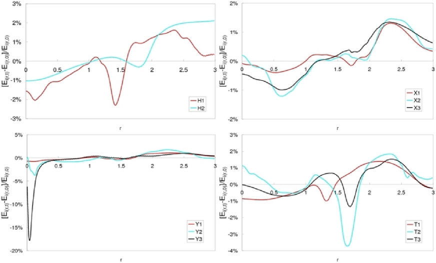
Figure 10: Fractional change in internal energy $(E_{i(r,t)}-E_{i(r,0)})/E_{i(r,0)}$ as a function of spherical radius from the center of the cluster between final and initial states, scaled by the corresponding initial internal energy for all 9 MHD and two hydrodynamical runs. Panels are (from right to left, and from top to bottom): hydrodynamic runs H1 and H2, horizontal field runs X1, X2, and X3, vertical field runs Y1, Y2, and Y3, and toroidal field runs T1, T2, and T3.

It is difficult to assess the implications of these results on the long term thermal stability of the ICM. Our simulations follow the dynamical evolution of one bubble over roughly 100 Myr, rather than an ensemble of bubbles produced by jet activity over cosmological timescales. Nevertheless, our results show that the most realistic field geometries (e.g. toroidal field within the bubble) produces a net heating of a few percent in the outer regions. None of our simulations produces strong heating in the inner regions, where the cooling times are shortest.

5 Conclusions

We have studied the buoyant rise of bubble including the effect of magnetic fields and anisotropic (Braginskii) viscosity. Our primary conclusions are the following:

1. Both strong magnetic fields and anisotropic viscosity have similar effects on the evolution of rising bubbles. They both can suppress instabilities in the direction parallel to the field, while having little effect on interchange instabilities that develop perpendicular to the field.

2. The detailed evolution of the bubble depends on the initial field direction. A toroidal field confined to the bubble interior produces structures that are most consistent with observed cavities and filaments.

3. Rising bubbles do not dramatically alter the initial structure of strong magnetic fields. In particular, strong horizontal fields remain mostly horizontal even after the passage of the bubble, as measured by the ratio of the magnetic energy in the vertical as compared to the horizontal component of the field.

4. All the models we have run show an increase in the internal energy (heating) of a few percent in the outer regions at late time, and a decrease in the internal energy (cooling) in the region below the bubble. Our simulations do not show that buoyant bubbles are an effective mechanism for heating the ICM in the central regions of the cluster.

The primary limitation of our study is that we neglect several physical processes that are likely to be important in real clusters. We do not follow the inflation of the bubble by an AGN self-consistently, rather we study the buoyant evolution of a bubble initially at rest in the ICM. It is possible that the transient evolution associated with the initial upward acceleration of the bubble will affect the resulting stability and mixing, thus it is more realistic to follow the inflation of the bubble directly (Pizzolato & Soker 2006). Furthermore, we study mostly uniform magnetic fields, whereas the field in real clusters is likely to be highly tangled. Finally, we have neglected the effect of thermal conduction, cosmic rays, and turbulent motions in the ICM driven by merger of substructures. Nevertheless, our idealized models allow us to isolate the effect of specific physics, namely magnetic fields and anisotropic viscosity, on the dynamics of the ICM. We find that both have a significant effect, and should be included in more realistic studies.

In the future, it would be productive to study the interaction of jets with the ICM directly. It is likely that adaptive mesh refinement (AMR) simulations that can simultaneously resolve the jet and global cluster structure will be required. Our results indicate it will be necessary to include the effects of MHD and anisotropic transport coefficients in such models to capture the physics of the ICM correctly.

References

- Balbus (2000) Balbus S.A., 2000, ApJ, 534, 420
- Balbus (2004) Balbus S.A., 2004, ApJ, 616, 857
- (3) Basson J.F. & Alexander P., 2003, MNRAS, 339, 353
- Birzan et al. (2004) Birzan, L., Rafferty, D. A., McNamara, B. R., Wise, M. W., Nulsen, P. E. J., 2004, ApJ, 607, 800
- Bogdanovic et al. (2009) Bogdanovic T., Reynolds C. S., Balbus S., Parrish I., 2009, arXiv:0905.4508v2
- Bruggen (2003) Bruggen M., 2003, ApJ, 592, 839
- Bruggen & Kaiser (2001) Bruggen M. & Kaiser C.R., 2001, MNRAS, 325, 676
- Bruggen & Kaiser (2002) Bruggen M. & Kaiser C.R., 2002, Natur, 418, 301
- Bruggen et al. (2009) Bruggen M., Scannapieco E., Heinz S., 2009, MNRAS, 395, 2210
- Carilli et al. (1994) Carilli C.L., Perley R.A., & Harris, D.E., 1994, MNRAS, 270, 173
- Carilli & Taylor (2002) Carilli C.L. & Taylor G.B, 2002, ARA&A, 40, 319
- Chandrasekhar (1961) Chandrasekhar S., 1961, Hydrodynamic and Hydromagnetic Stability (Oxford: Clarendon)
- Churazov et al. (2001) Churazov E., Br ggen M., Kaiser C. R., Bohringer H., Forman W. 2001, ApJ, 554, 261
- Diehl et al. (2008) Diehl S., Li H., Fryer C. L., Rafferty D., 2008, ApJ, 687, 173
- Dursi $ Pfrommer (2008) Dursi L. J. & Pfrommer C., 2008, ApJ, 677, 993
- Fabian (1994) Fabian A. C., 1994, ARA&A, 32, 277
- Fabian et al. (2000) Fabian A. C., Sanders J. S., Ettori S., Taylor G. B., Allen S. W., Crawford C. S., Iwasawa K., Johnstone R. M., Ogle P. M., 2000, MNRAS, 318, L65
- Fabian et al. (2003) Fabian A. C., Sanders J. S., Allen S. W., Crawford C. S., Iwasawa K., Johnstone R. M., Schmidt R. W., Taylor G. B., 2003, MNRAS, 344, L43
- Fabian et al. (2005) Fabian A. C., Reynolds C. S., Taylor G. B., Dunn R. J. H., 2005, MNRAS, 363, 891
- Gardini (2007) Gardini A., 2007, A& A, 464, 143
- Gardini & Stone (2005) Gardini T.A. & Stone J.M., 2005, JCoPh, 205, 509
- Gardini & Stone (2008) Gardini T.A. & Stone J.M., 2008, JCoPh, 227, 4123
- Islam & Balbus (2005) Islam T. & Balbus S., 2005, ApJ, 633, 328
- Jones & De Young (2005) Jones T.W. & De Young D.S., 2005, ApJ, 624, 586
- Liu (2008) Liu W., Li H., Li S., Hsu S. C., 2008, ApJ, 684, L57
- Lyutikov (2007) Lyutikov M. 2007, ApJ, 668, L1
- Lyutikov (2008) Lyutikov M. 2008, ApJ, 673, L115
- McNamara et al. (2000) McNamara B.R., et al. 2000, ApJ, 534, L135
- Nakamura et al. (2006) Nakamura M., Li H., Li S., 2006, ApJ, 652, 1059
- Nakamura et al. (2007) Nakamura M., Li H., Li S., 2007, ApJ, 656, 721
- Omma et al. (2004) Omma H., Binney J., Bryan G., Slyz A., 2004, MNRAS, 348, 1105
- O’Neill et al. (2009) O’Neill S. M., De Young D. S., Jones T. W., 2009, ApJ, 694, 1317
- Parrish & Stone (2005) Parrish I. J. & Stone J.M., 2005, ApJ, 633,334
- (34) Parrish I. J. & Stone J.M., 2007, AP&SS, 307, 77
- (35) Parrish I. J. & Stone J.M., 2007, ApJ, 633,334
- Parrish & Quataert (2008) Parrish I. J. & Quataert E., 2008, ApJ, 677, L9
- Parrish et al. (2008) Parrish I. J., Stone J. M., Lemaster N., 2008, ApJ, 688, 905
- Parrish et al. (2009) Parrish I. J., Quataert E., Sharma P., 2009, ApJ, 703, 96
- Pavlovski et al. (2008) Pavlovski G., Kaiser Christian R., Pope E. C. D., Fangohr H, 2008, MNRAS, 384, 1377
- Peterson & Fabian (2006) Peterson J. R. & Fabian A.C. 2006, Phys. Tep., 427, 1
- Pizzolato & Soker (2006) Pizzolato F. & Soker N., 2006 MNRAS, 371, 1835
- Quataert (2008) Quataert E., 2008, ApJ, 673, 758
- Quilis et al. (2001) Quilis V., Bower R. G., Balogh M. L., 2001, MNRAS, 328, 1091
- Reynolds et al. (2002) Reynolds C. S., Heinz S., Begelman M.C., 2002, MNRAS, 332, 271
- Reynolds et al. (2005) Reynolds C. S., McKernan B., Fabian A. C., Stone J. M., Vernaleo J. C., 2005, MNRAS, 357, 242
- Robinson et al. (2004) Robinson K., et al., 2004, ApJ, 601, 621
- Ruszkowski et al. (2004) Ruszkowski M., Bruggen M., Begelman M. C., 2004, ApJ, 615, 675
- Ruszkowski et al. (2007) Ruszkowski M., Enlin T. A., Bruggen M., Heinz S., Pfrommer C., 2007, MNRAS, 378, 662
- Scannapieco & Bruggen (2008) Scannapieco E., Bruggen M., 2008, ApJ, 686, 927
- Sharma et al. (2006) Sharma P., Hammett G. W., Quataert E., Stone J. M. 2006, ApJ, 637, 952
- Sharma & Hammett (2007) Sharma P. & Hammett G. W., 2007, JCoPh, 227, 123
- Sharma et al. (2009) Sharma P., Chandran B. D. G., Quataert E., Parrish, I. J. 2009, ApJ, 699, 348
- Spitzer (1962) Spitzer, L. 1962, Physics of Fully Ionized Gases (Physics of Fully Ionized Gases, New York: Interscience (2dn edition), 1962)
- Sternberg et al. (2007) Sternberg A., Pizzolato F. & Soker N. 2007, ApJ, 656, 5
- Sternberg & Soker (2009a) Sternberg A. & Soker N. 2009 MNRAS 395, 228
- Sternberg & Soker (2009b) Sternberg A. & Soker N. 2009 MNRAS 398, 422
- Stone et al. (2008) Stone J. M., Gardiner T. A., Teuben P., Hawley J. F., Simon J. B. 2008, ApJ, 178, 137
- (58) Stone J.M., & Gardiner, T.A. 2007, Phys. Fluids, 19, 4104.
- (59) Stone J.M., & Gardiner, T.A. 2007, ApJ, 671, 1726
- Stone & Balbus (2009) Stone J.M., & Balbus, S.A. 2009, in preparation.
- Shore (1992) Shore S.N., 1992, An Introduction to Astrophysical Hydrodynamics (New York: Academic)
- Taylor et al. (2002) Taylor G.B., Fabian A.C., Allen S.W., 2002, MNRAS, 334, 769
- Young et al. (2002) Young A. J., Wilson A. S., & Mundell C. G., 2002, ApJ, 579, 560