Low Resolution Spectral Templates For AGNs and Galaxies From 0.03 – 30$\mu$m

Abstract

We present a set of low resolution empirical SED templates for AGNs and galaxies in the wavelength range from 0.03 to 30$\mu$m based on the multi-wavelength photometric observations of the NOAO Deep-Wide Field Survey Boötes field and the spectroscopic observations of the AGN and Galaxy Evolution Survey. Our training sample is comprised of 14448 galaxies in the redshift range $0\lesssim z\lesssim 1$ and 5347 likely AGNs in the range $0\lesssim z\lesssim 5.58$. The galaxy templates correspond to the SED templates presented by Assef et al., (2008) extended into the UV and mid-IR by the addition of FUV and NUV GALEX and MIPS 24$\mu$m data for the field. We use our templates to determine photometric redshifts for galaxies and AGNs. While they are relatively accurate for galaxies ($\sigma_{z}/(1+z)=0.04$, with 5% outlier rejection), their accuracies for AGNs are a strong function of the luminosity ratio between the AGN and galaxy components. Somewhat surprisingly, the relative luminosities of the AGN and its host are well determined even when the photometric redshift is significantly in error. We also use our templates to study the mid-IR AGN selection criteria developed by Stern et al., (2005) and Lacy et al. (2004). We find that the Stern et al., (2005) criteria suffers from significant incompleteness when there is a strong host galaxy component and at $z\simeq 4.5$, when the broad H$\alpha$ emission line is redshifted into the [3.6] band, but that it is little contaminated by low and intermediate redshift galaxies. The Lacy et al. (2004) criterion is not affected by incompleteness at $z\simeq 4.5$ and is somewhat less affected by strong galaxy host components, but is heavily contaminated by low redshift star forming galaxies. Finally, we use our templates to predict the color-color distribution of sources in the upcoming WISE mission and define a color criterion to select AGNs analogous to those developed for IRAC photometry. We estimate that in between $640,000$ and $1,700,000$ AGNs will be identified by these criteria, but without additional information, WISE-selected quasars will have serious completeness problems for $z\gtrsim 3.4$.

1 Introduction

Upcoming large photometric surveys like the ground based LSST (Tyson, 2002), Pan-STARRS (Kaiser, 2004), DES (The Dark Energy Survey Collaboration, 2005) and UKIDSS (Lawrence et al., 2007) projects, or the space-based WISE (Mainzer et al., 2005) mission, will increase the number of cataloged sources in the universe by a large factor. Most objects always lie at the survey magnitude limit, which means that spectroscopic follow-up will only be possible for a small fraction of objects, and much of the science will need to rely solely on multi-wavelength photometric observations. One of the main tools for analyzing the multi-wavelength photometry is the modeling of the spectral energy distributions (SED) of the sources. SEDs can be used to estimate photometric redshifts and K-corrections, to study luminosity functions and the properties of different populations of objects, and to select smaller subsamples for follow-up studies.

Galaxy SEDs have been studied using many different techniques. Theoretical models based on population synthesis of stellar spectra (e.g. Bruzual & Charlot,, 2003; Fioc & Rocca-Volmerange, 1997; Leitherer et al., 1999) have been successfully applied in many studies of galaxies. Their strength is that they allow the estimation of physically relevant parameters, like star formation rates, ages, masses and metallicities solely by comparing the SED models to the photometric observations. However, there are unknowns in the spectral properties of stars and stellar populations, such as the presence of thermally pulsating AGB stars (e.g. Conroy et al., 2009) and the effects of binaries (Eldridge & Stanway, 2009), as well as non-stellar sources of emission, such as dust in the interstellar medium (ISM) or active nuclei, and absorption, both broadly distributed and associated with stars, that alter or modify the SEDs. Some of these issues can be avoided by the use of empirical SED templates (e.g. Coleman, Wu & Weedman,, 1980; Kinney et al., 1996; Devriendt, Guiderdoni & Sadat,, 1999; Assef et al.,, 2008). However, most empirical templates lack the broad wavelength coverage of the theoretical ones.

Almost all AGN SED templates are empirical, as the physical processes governing AGN emission are not quantitatively understood. Elvis et al. (1994) constructed the mean SED of Type 1 AGNs by combining spectroscopic redshifts and multi-wavelength photometric observations ranging from the radio to the X-rays of 47 known quasars. A similar approach was followed by Richards et al., (2006) over a similar wavelength range based on 259 SDSS Type 1 AGNs. Both studies, however, include a limited number of AGNs, do not consider reddening and do not self-consistently model contamination from the host galaxy.

In a previous paper (Assef et al.,, 2008, hereafter A08) we presented a set of empirical galaxy templates derived from the extensive photometric observations of the NOAO Deep Wide-Field Survey (NDWFS; Jannuzi & Dey, 1999) Boötes field and their spectroscopic follow up observations by the AGN and Galaxy Evolution Survey (AGES; Kochanek et al., in prep., ). These templates form a linear non-negative basis for the color-color space spanned by galaxies and accurately reproduce SEDs in the wavelength range from 0.2 to 10$\mu$m. Here, we extend that work in two different directions. First, we extend the wavelength range from 0.03 to 30 $\mu$m by incorporating GALEX UV (Martin et al.,, 2005) and MIPS 24$\mu$m (Weedman et al.,, 2006) observations, and secondly, we add a template for AGN emission derived in the same manner as the galaxy templates. By simultaneously deriving the AGN and galaxy SEDs, we self-consistently account for the host contamination. We also correct for the reddening of the different AGNs in our sample. Because AGES selects AGN using a broad range of selection methods, our AGN template is not exclusively applicable to unreddened Type 1 quasars. Earlier versions of this extended set of templates have already been used by Atlee et al. (2009) as a part of a study of the evolution of the UV upturn in elliptical galaxies, and by Ross et al. (2009) to study the resolved host of the $z=1.7$ gravitationally lensed quasar SDSS J1004+4112. The latter study helped to verify that our models could correctly separate host and AGN contributions for unresolved systems.

This paper is structured as follows. In §2 we describe our photometric and spectroscopic data set. The algorithms we use to obtain the SED templates are discussed in §3, as well as the algorithm to use them for estimating photometric redshifts. In §4 we discuss our SED templates and their accuracy for estimating photometric redshifts of galaxies and AGNs, and we apply them to study the problems of mid-IR QSO selection in the IRAC bands and in the upcoming WISE satellite mission. In a subsequent paper (Assef et al.,, 2009, Paper II) we use these templates to study the IRAC-selected QSO luminosity function and its evolution with redshift. Throughout the text we assume a $\Lambda$CDM cosmology with $H_{0}=73~{}\rm km~{}\rm s^{-1}~{}\rm Mpc^{-1}$, $\Omega_{\rm M}=0.3$ and $\Omega_{\Lambda}=0.7$.

2 Data

The data used in this work are an expansion over that of A08. It is based on the extensive multi-wavelength imaging of the NOAO Deep Wide-Field Survey (NDWFS; Jannuzi & Dey, 1999) Boötes field and the spectroscopic observations of the same field by the AGN and Galaxy Evolution Survey (AGES; Kochanek et al., in prep., ). NDWFS is a deep optical and near-infrared survey that covers two 9.3 deg² regions of the sky, the Boötes and Cetus fields. We focus on the Boötes field, which was imaged in $B_{W}$ (3500-4750 Å, peak at $\approx 4000$ Å), $R$, $I$ and $K$ pass-bands to depths of approximately 26.5, 26, 25.5 and 21 AB magnitudes ($5\sigma$, 2^′′ diameter aperture). Extensive follow-up imaging of the field at different wavelengths has been obtained by several other surveys. In particular we include $J$ and $K_{s}$ data from the Flamingos Extragalactic Survey (FLAMEX; Elston et al.,, 2006), $z^{\prime}$ data from zBoötes (Cool, 2007), MIPS 24$\mu$m data from Weedman et al., (2006), NUV and FUV observations from the GALEX GR5 release (Morrissey et al., 2007), and the mid-IR IRAC observations of the Spitzer Deep-Wide Field Survey (SDWFS; Ashby et al., 2009). The IRAC Shallow Survey (Eisenhardt et al., 2004), which we used in A08, is a subset of the SDWFS data. While in A08 we referred to the IRAC channels by C1, C2, C3 and C4 for the 3.6, 4.5, 5.8, and 8$\mu$m bands, here we will use the more common nomenclature with the channel’s wavelength in square brackets ([3.6],[4.5],[5.8] and [8.0]). It should be noted that there are also radio (FIRST: Becker et al., 1995; WENSS: Rengelink et al., 1997; WSRT: de Vries et al., 2002; NVSS: Condon et al., 1998) and X-ray (Chandra XBoötes: Murray et al., 2005) observations of the field that we do not directly include in our analysis.

AGES is a redshift survey in the NDWFS Boötes field using the 300 fiber robotic Hectospec instrument (Fabricant et al.,, 2005) on the 6.5m MMT telescope. AGES obtained spectra for $\approx 26000$ objects in the wavelength range from 3200 to 9200Å. Spectroscopic redshifts have been measured for about 18000 galaxies in the redshift range from 0 to 1 with a magnitude limit of $I=20$, and about 7000 likely AGNs in the range from 0 to 6 up to $I=22.5$. Because of the different magnitude limits for the samples, AGN candidates were pre-selected from the photometric observations. A source was targeted as an AGN if it met any of the following criteria:

• X-Ray: The object was detected in X-rays by XBoötes. The contaminants in the X-ray sample are primarily active stars, along with a small number of very low redshift early and late type galaxies (see e.g. Stern et al., 2002, for a description of the origin of X-ray emission in galaxies).

• Radio: The object has an associated unresolved $5\sigma$ WSRT detection. Radio emission is generally associated with AGNs, but can also be due to star formation at low radio powers (e.g. Hickox et al., 2009; Kauffmann et al., 2008). Strongly star forming galaxies at low redshift can contaminate this sample.

• MIPS: The object was detected in the 24$\mu$m MIPS images with a flux $F>0.3$ mJy, appears as a point source in the optical data and has an $I$-band magnitude fainter than $18-2.5\log(F/\rm mJy)$. This $I$-band magnitude limit eliminates normal stars. The MIPS sample is contaminated by star forming galaxies that are classified as point sources in the optical photometry.

• IRAC: The object has IRAC colors that suggest the presence of an AGN. The exact color-color boundaries and magnitude limits vary between optical point and extended sources that are discussed in detail in Paper II, but are based on modified versions of the Stern et al., (2005) criterion.

The final AGES sample includes spectra for 3047, 789, 2025 and 3844 objects targeted as AGN by the X-ray, radio, MIPS and IRAC criteria respectively.

After the observations, spectra were analyzed using a modified version of the SDSS spectral pipeline. Based on the template fits to the spectra, objects that showed clear signatures of nuclear activity were classified as spectroscopic AGNs. This classification has limits, as obscured AGN may lack optical signatures of activity, and the pipeline classifications emphasize the presence of broad lines over the more subtle classification problems for narrow lines. For narrow line sources we also used the emission line classifications of Moustakas et al. (2009). We view these various AGN classifications as complimentary rather than focusing only on one.

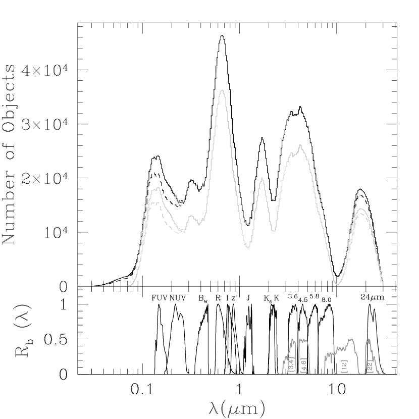
Figure 1: (Upper panel) The wavelength coverage of our data set (black), as described in §2. The solid line shows the coverage when photometry upper limits are included while the dashed line only considers detections. We also show both histograms for the sample used to construct the galaxy SED templates alone (gray) which excludes AGNs (see §3.1). (Bottom panel) Filter sensitivity curves for all bands included in our data set are shown by the solid black lines. Filter sensitivity curves for the upcoming WISE mission are shown by the dark gray solid lines at half-height to distinguish them from the other bands.

When possible, we have added upper limits to all objects observed, but not detected, in the UV, optical, near-IR and 24$\mu$m. The catalog from which we build the SED templates consists of all objects that have been detected, or have upper limits, in at least 8 of the 14 bands available (FUV, NUV, $B_{W}$, $R$, $I$, $z^{\prime}$, $J$, $Ks$, $K$, [3.6], [4.5], [5.8], [8.0] and 24$\mu$m) and which have a reliable redshift measured by AGES. We eliminate objects close to bright stars. The minimum number of bands is required to guarantee that all SED fits have at least 2 degrees of freedom (see §3). Our final data set comprises 19795 objects, of which 14448 are nominally “pure” galaxies with no signs of nuclear activity and 5347 show some type of AGN signature. On average, each object has been detected in 10 of the 14 available bands, and Figure 1 shows the rest-frame wavelength coverage of our final sample.

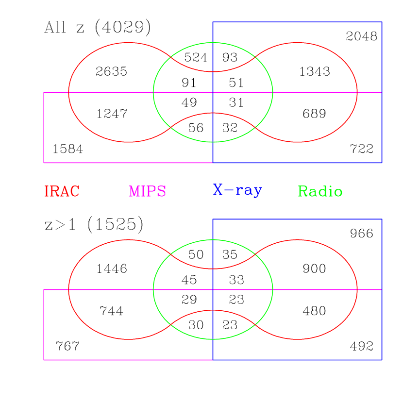
Figure 2: Edwards representation of a four set Venn diagram showing the number of AGNs selected by each photometric criteria and the overlap between them. The top panel shows this for our full sample while in the bottom panel we have restricted it to objects with $z>1$ in order to show how the photometric selection criteria overlap in a contamination free, but limited, sample. Note that in each panel there are four geometrical figures, each representing a photometric selection criteria: MIPS (magenta rectangle), X-ray (blue rectangle), radio (green circle) and IRAC (red “peanut” shaped region). The intersection between the regions show the number of objects targeted simultaneously by each combination of criteria.

Figure 2 shows a Venn diagram representation of the 4029 photometrically selected AGNs in our sample. Each geometrical shape represents a different photometric selection criteria, and the intersections between them show the number of objects targeted simultaneously by each of those criteria. The rest of the AGNs in our sample are spectroscopically confirmed by their line ratio classification of Moustakas et al. (2009, 1242 objects in total of which 1034 do not meet any photometric targeting criteria) or by the analysis of the spectroscopic pipeline (2418 objects in total of which 268 were not targeted by their photometry and were not classified as Type 2 AGNs by Moustakas et al. 2009). The remaining 16 active objects were targeted by their optical colors using a selection technique of minor importance in the AGES survey. Figure 2 also shows the Venn diagram representation of all $z>1$ objects, in order to show how the photometric selection criteria overlap in the absence of contaminants. Notice, however, that each selection criteria has different redshift-dependent biases, so the differences between the two Venn diagrams are not solely due to contaminating inactive galaxies.

3 Methods

The methods we use to derive the SED templates and estimate photometric redshifts follow closely those described in A08. In this section we give a brief summary of how our methods work and we detail the changes we have made to the original algorithms. We refer the reader to A08 for a detailed discussion of the latter.

3.1 Templates

We assume that the spectrum of any object in our sample can be modeled as a linear combination of a small set of unknown spectral templates. We construct these templates by using the data described in §2. For “pure” galaxies, we assume the majority of them have SEDs that can be described as a linear combination of three templates: one similar to an elliptical galaxy (an old stellar population), one similar to a spiral galaxy (a continuously star forming population), and a third similar to an irregular galaxy (a starburst population). For objects with active nuclei, a population that was not included in the analysis of A08, we assume that every AGN SED can be described by the same spectral template with varying amounts of reddening and absorption by the intergalactic medium (IGM), combined with the galaxy templates to describe the host. We assume the reddening follows an SMC-like extinction curve for $\lambda<3300$Å and a Galactic extinction curve at longer wavelengths, assuming $R_{V}=3.1$ for both. This is based on the observed absence of the Galactic 2175Å feature of Galactic extinction curves in QSO spectra (e.g. York et al., 2006). For the SMC reddening law we assume the functional form derived by Gordon & Clayton (1998) using the star AzV 18, while for the Galactic reddening we assume the functional form of Cardelli et al. (1989). The IGM absorption is applied to all templates and not solely the AGN one, but it is most important for the AGN due to their high redshifts. We model the IGM absorption following Fan et al., (2006) for Ly$\alpha$ and Ly$\beta$ absorption, and Stengler-Larrea et al., (1995) for Lyman limit systems. We leave the strength of absorption as a free parameter of the model in order to allow for variations in absorption between objects. We only include the IGM absorption component for redshifts above 0.8, as below this redshift Ly$\alpha$ falls outside of our wavelength coverage. To force every combination of these four templates to be physically plausible, we require the SED of every object to be a non-negative linear combination of these templates.

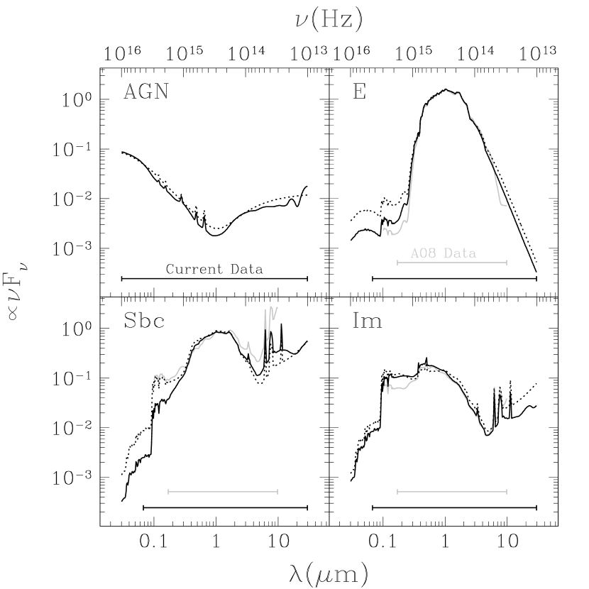
Figure 3: Resulting best fit templates from applying the algorithm of §3.1 to the data set described in §2 (black solid) compared to their initial guesses (black dotted) and to the templates derived in A08 (gray solid). Note that the bottom axis of each panel shows wavelength while the top shows frequency. The bars at the bottom of each panel show the rest-frame wavelength coverage of our data set (black, see Fig. 1) and of that used in A08 (gray).

Our algorithm is iterative (see discussion below and §3.1 of A08, ) and hence we must start from an initial guess and sequentially improve it to best fit the data at each iteration. For the galaxy templates, we start from the Coleman, Wu & Weedman, (1980) E, Sbc and Im template for the “elliptical”, “spiral” and “irregular” components, extended into the UV and IR by the Bruzual & Charlot, (2003) stellar synthesis models. Because the models of Bruzual & Charlot, (2003) do not consider dust or PAH emission, which are critical in the mid-infrared for the star forming templates, we added ad-hoc linear combinations of the mid-infrared part of the VCC1003 (NGC 4429) and M82 SEDs obtained by Devriendt, Guiderdoni & Sadat, (1999) to the Sbc and Im templates. For the AGN template we consider two different starting points: an ad-hoc template constructed from different observational and theoretical considerations, and the average Type 1 quasar SED of Richards et al., (2006). The ad-hoc template consists of a combination of modified power-laws that resemble the large scale behavior of the Richards et al., (2006) Type 1 quasar mean energy distribution in the IR and optical, modified in the UV to fall as predicted by a simple accretion disk model, and with the addition of the broad-spectral lines of an AGN. We choose to make our initial template as blue in the optical as our bluest AGNs, which is significantly bluer than the Richards et al., (2006) SED. The shape of this template, along with the initial guess for our galaxy templates, is shown in Figure 3. Our results refer to this starting model except where noted otherwise. While the two model templates produce very similar results, we prefer the ad-hoc starting point because the Richards et al., (2006) SED has considerable amounts of host contamination (see §4.1).

Each template is divided into 300 uniformly logarithmically spaced wavelength bins extending from 0.03 to 30$\mu$m, hence the “low resolution”. Each bin is then directly fit to the data using $\chi^{2}$ minimization over the entire calibration sample. Because this is still a significantly higher resolution than the width of the broad-band filters, we add a smoothing term ($H$) to the $\chi^{2}$ minimization that penalizes departures from the smoothness of the initial guesses. Note that this resolution is higher than that used in A08. In summary, we optimize the function

$$G\ =\ \chi^{2}\ +\ \frac{1}{\eta^{2}}H.$$ (1)

The $\chi^{2}$ term is given by

$$\chi^{2}\ =\sum_{i,b}\left(\frac{F_{i,b}-F^{\rm mod}}{\sigma_{i,b}}\right)^{2},$$ (2)

where indices $i$ and $b$ enumerate objects and bands respectively, $F$ is the observed flux, $F^{\rm mod}$ is the template model flux and $\sigma_{i,b}$ is the photometric error. We defined the smoothing term $H$ to be

$$H\ =\ \sum_{k,n}\left(\log{\frac{T_{k,\nu_{n}}}{Q_{k,\nu_{n}}}}-\log{\frac{T_{k,\nu_{n+1}}}{Q_{k,\nu_{n+1}}}}\right)^{2},$$ (3)

where $T_{k,\nu_{n}}$ is the flux per unit frequency of SED template $k$ in wavelength bin $n$ (frequency $\nu_{n}$), and $Q_{k,\nu_{n}}$ is the corresponding value in our initial template guess. For a detailed discussion of these terms, we refer the reader to A08. For galaxies, we use $\eta=0.002$, which is half of that used in A08 due to the increased resolution, but the results are not very sensitive to this choice. For the AGN template we increased the value to $\eta=0.005$ as the amplitude of the changes is much smaller than for galaxies.

The equations for optimizing equation (1) are linear in all parameters but the AGN reddening and the IGM absorption. To solve the linear equations while imposing the condition that the contribution of each template to each SED must be strictly non-negative and that at every wavelength the templates must be positive, we use a simple non-negative least square solver.

To summarize, our algorithm proceeds as follows: (1) we estimate the contribution of each template to the SED of each object; (2) we estimate the zero point correction to each photometric band; (3) we sequentially optimize the templates; (4) return to step (1). Note that when optimizing a given template we only use objects with at least a 20% contribution from the template to the integrated luminosity of its best fit SED in the previous step. Since the 24$\mu$m data are effectively decoupled from the rest of the data (see Fig. 1), we cannot fit a zero-point correction to this channel. For this reason, unlike in A08, we do not attempt to remove the large scale behavior of the zero point corrections. Instead, we include a Gaussian prior to penalize unnecessary modifications to the zero points, with a dispersion of 1% for all bands except the MIPS 24$\mu$m channel.

We first derive the best fit galaxy SED templates without the AGN template by using only objects that show no signatures of nuclear activity. To be conservative, we eliminate all objects photometrically targeted as AGNs by AGES, all objects for which the SDSS pipeline finds an AGN component in the spectrum, and all objects classified as narrow line AGNs by Moustakas et al. (2009) (see §2). We then fit the AGN template by using our full sample while keeping the galaxy templates fixed. When determining the galaxy templates, we eliminate the 3% of the objects with the poorest fits, while for determining the AGN template we eliminate the worst 5%. These are mostly objects with either bad data points or galaxies with unflagged nuclear activity.

3.2 Photometric Redshifts

For photometric redshifts we follow the same basic steps as those in A08. We perform a $\chi^{2}$ minimization similar to that outlined in §3.1, solving all linear equations with the NNLS algorithm combined with a grid of reddening values for the AGN template as a function of redshift. The main difference is that we fix the IGM absorption to a typical value rather than letting it vary (see §4.2 for a discussion of this point). For optimizing the photometric redshifts, we also include a luminosity prior based on the Las Campanas Redshift Survey (Lin et al.,, 1996) luminosity function that only affects the galaxy templates (with and without and AGN component on the SED). The shape and specific parameters of the prior probability function are discussed in detail in A08. Our publicly available algorithms for estimating photometric redshifts have been updated to reflect these changes and include the new templates.

4 Results

In this section we describe the SED templates resulting from applying the algorithm discussed in §3.1 to the data set described in §2 and we also discuss their application to determining photometric redshifts for AGNs and galaxies, and to study the mid-IR selection of QSOs in the IRAC bands and in the upcoming WISE satellite mission.

4.1 Templates

The final templates are shown in Table 1 and in Figure 3. Table 2 shows the absolute magnitudes of the templates as a function of redshift in various photometric bands including those of our sample. Figure 3 also shows the initial guesses from which the process started. The galaxy templates show significant departures from the initial ones, just as in A08. In particular, the elliptical template is significantly redder in the UV and somewhat bluer in the mid-IR. The spiral-like template has decreased UV and a increased dust/PAH emission relative to the 1.6$\mu$m stellar emission peak. The Im template shows a somewhat decreased UV and mid-IR continuum relative to the near-IR peak. The departures from the initial templates are caused by a combination of changes in the balance of the underlying stellar populations and by their inability to reproduce the SEDs of galaxies, either because of missing physics or, in the mid-IR, because of the ad hoc addition of dust emission used to create them (see §3.1 for details).

The AGN template based on our ad-hoc model also shows significant differences from the initial guess. In particular, the optical is bluer and the mid-IR is redder. At longer wavelengths ($\gtrsim 15\mu\rm m$), the template shows a steep rise, but this is likely to be an artifact caused by the lack of $z=0$ quasars to constrain this wavelength region. At wavelengths shortward of Ly$\alpha$, the templates cannot be constrained, as the observed SEDs are completely dominated by IGM absorption. Since the flux in X-rays is generally significantly lower than the UV emission in AGNs, as determined by the values of $\alpha_{OX}$ (e.g. Tananbaum et al., 1979; Strateva et al., 2005), we know the spectrum must turn down at some wavelength shortward of Ly$\alpha$. For this reason, we choose in the rest of the paper to estimate “bolometric” luminosities by integrating our AGN template only at wavelengths longward of Ly$\alpha$.

Using the average SED of Type 1 quasars derived by Richards et al., (2006) as a starting point for our AGN template yields similar results, albeit with some interesting differences. The AGN template resulting from this starting point is shown in Figure 4, as compared to the original Richards et al., (2006) template and our “standard” template. Relative to the initial template, the converged template is somewhat brighter in the UV relative to the optical and near-IR wavelengths. The mean color is a combination of extinction and any dependence of the SED on black hole mass and accretion rate (e.g. Yip et al., 2004). While our algorithm corrects for the former, it can mimic the latter using small amounts of reddening. In the optical wavelengths, the contribution from broad emission lines to the Richards et al., (2006) template is heavily smoothed by the averaging of the broad band photometry used to build it, however the output template to our algorithm has developed much sharper emission line features. The minimum in the near-IR of the converged template has shifted to a shorter wavelength, as also seen in our “standard” template. This is likely due to our self-consistent treatment of the host. At $\sim 4.5\mu$m there is a depression in the SED. It is unclear if this is a real feature or not, as it does not appear in our standard AGN template. The differences at the longest wavelengths and wavelengths shorter than Ly$\alpha$ are not significant due to the lack of data needed to constrain these regions (see Fig. 1 and the discussion in the previous paragraph). When combined with the host galaxy templates, both AGN templates work well, suggesting that the main difference is that the Richards et al., (2006) template intrinsically has more host contamination than our standard template, which can be compensated for by changing the amount of host galaxy template added to fit an object. This can be seen in Figure 5, which shows that the values of $L_{\rm AGN}/L_{\rm Host}$ are, in average, $\approx 35\%$ larger for the converged Richards et al., (2006) AGN template than for the standard template.

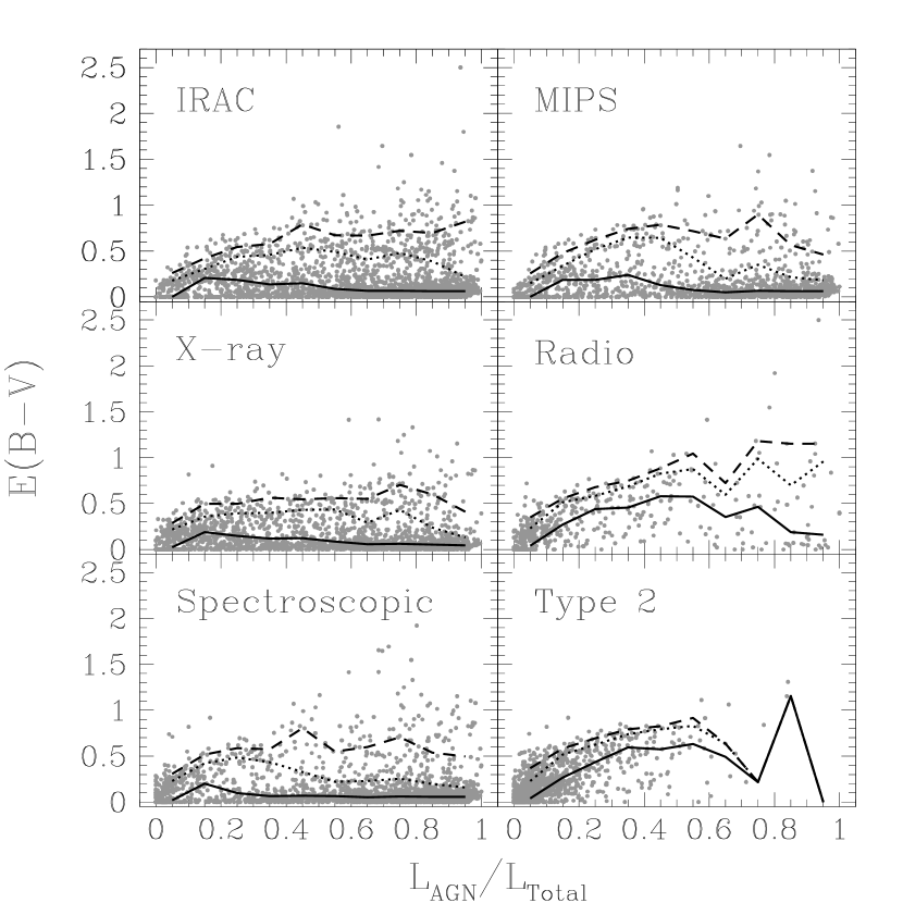
Figure 6: Best fit reddening to the AGNs in our sample as a function of the contribution of the AGN component to the total bolometric luminosity. The AGN luminosity has been corrected for the estimated extinction. The top and middle panels show the objects targeted as AGN candidates by AGES according to their photometric properties (see §2). The bottom left panel shows the reddening distribution for objects classified as AGNs by the spectroscopic pipeline while the bottom right panel shows it for the objects classified as Type 2 AGNs by Moustakas et al. (2009). In each panel, the solid black line shows the median E(B–V) as a function of $L_{\rm AGN}/L_{\rm Host}$ while the dotted and dashed lines show the 85% and 95% contours respectively.

In Figure 6 we show the best fit extinctions to the AGNs in our sample for our standard AGN template. Objects have been divided according to the criteria by which they were selected and objects targeted by multiple criteria are shown in all of the relevant panels. In all cases, there seems to be a maximum observed reddening that increases with increasing AGN luminosity relative to their hosts. This can be understood as a combination of three effects. One is that a more heavily reddened AGN needs to be more luminous relative to the host in order to meet many of the AGES AGN targeting criteria. The second effect is the inability of our templates to detect highly reddened AGNs with bright hosts and, if detected, to determine the reddening parameter with precision. If the host dominates the UV/optical/NIR wavelengths, reddening values above a certain threshold will not significantly affect the $\chi^{2}$ until they start to modify the mid-IR colors. Otherwise, our algorithm defaults to using the smallest possible reddening value. Finally, our sample is magnitude limited, and hence the more reddened, optically fainter objects can be found in a smaller physical volume than the less reddened, optically brighter ones. The first problem primarily affects the IRAC and MIPS targeting criteria, while the second and third ones affect all cases. Notice, however, that the X-ray selected objects are relatively unaffected by these biases. In Figure 6 we also see that the AGNs which are brightest in comparison to their hosts show a range of small, but positive, extinctions. This may be due to our algorithm using small amounts of reddening to compensate for changes in the SED with BH accretion rates and masses, as discussed above.

Figure 3 also shows the galaxy templates derived in A08. The elliptical and irregular templates show significant changes only in the UV and mid-IR, as would be expected from the addition of the GALEX and $24\mu$m MIPS data. The spiral template also shows departures at those wavelengths, but differences are also seen in the near- to mid-IR region. In our model the templates form a non-orthogonal basis that, due to the restriction to positive combinations, determine the boundaries of the color space occupied by galaxies. Changes in the templates are really changes in the boundaries of the permitted color space. We expect that the differences between the new and old templates over the wavelength range covered by the old templates can largely be explained by making the new/old templates linear combinations of the old/new templates. Note that the coefficients of the “rotation” can be negative. The best fit combination of our new templates to the E template of A08 is given by the coefficients (1.02, –0.01, 0.00), to the Sbc one by (–0.51, 1.51, 0.00) and to the Im one by (–0.04, 0.34 and 0.70), where each coefficient represents the contribution of our new E, Sbc and Im templates respectively. These combinations reproduce very well the full wavelength range of the A08 templates, showing that the differences with our new templates correspond to a simple rotation of the basis vectors rather than a fundamental modification.

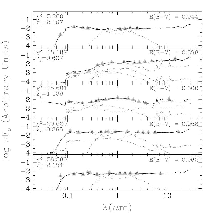
Figure 7: Best fit SEDs for four typical AGNs (top four panels) and for the AGN with the 90^th percentile worst $\chi^{2}_{\nu}$ in the sample (bottom panel). The solid line shows the best fit SED, which is composed of a non-negative combination of our optimized AGN (dotted), E (dashed), Sbc (long-dashed) and Im (dot-dashed) templates. In each panel we indicate the reddening applied to the AGN template. The flux of each filter, when detected, is shown by the solid triangles, while the open squares show the expectation from the best-fit. Arrows mark upper limits when they are available. The AGNs shown in the top four panels have SEDs typical of, from top to bottom, a Type 1, a Type 2, a very low luminosity AGN and a Type 1 with a very strong host component. For each object, the $\chi^{2}$ of the fit and the spectroscopic redshift measured by AGES is shown on the upper right corner of the corresponding panel.

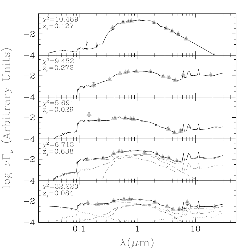
Figure 8: Best fit SEDs for four typical galaxies (top four panels) and for the galaxy with the 90^th worse $\chi^{2}_{\nu}$ in the sample (bottom panel). The different line styles and point types follow the same convention as in Figure 7. In the top four panels we show galaxies dominated by, from top to bottom, the elliptical, Sbc and Im templates, and a combination of all three.

Figures 7 and 8 show typical fits to AGNs and galaxies using the “standard” AGN template. These objects have $\chi^{2}$ values close to the median of their respective samples (median $\chi^{2}_{\nu}=1.35$ for galaxies and 2.60 for AGNs) and have been selected to show a range of different scenarios. The bottom panel of each Figure also shows the object with the 90^th percentile worst $\chi^{2}_{\nu}$ of each sample. Although small discrepancies are present at some wavelengths, the agreement is still generally very good. The vast majority of the objects in our sample are well described by our four templates. The converged Richards et al., (2006) template gives similar values of median $\chi^{2}_{\nu}$ (1.30 and 2.61 for galaxies and AGNs respectively) to our standard template as we would hope, given that our results should depend little on the priors.

In the following sections, we will explore different applications of our templates. We will study the accuracy of photometric redshifts from these templates for galaxies and AGNs, and the colors of these objects in the mid-IR bands of both IRAC and the upcoming WISE mission. In a subsequent paper (Paper II) we examine the AGN luminosity function and its evolution with redshift. Our templates also allow for the study of host properties in AGNs but this will be explored in an upcoming paper.

4.2 Photometric Redshifts

In this section we study the application of these templates to the estimation of photometric redshifts for galaxies and AGNs. To quantify their accuracy, we derive photometric redshifts for all the sources in the catalog used to build the templates, each of which has a measured spectroscopic redshift. As mentioned previously, for photo-zs we do not allow the IGM absorption strength parameter to vary, as allowing variations worsens the redshift accuracy, and we include a luminosity prior based on the Las Campanas Redshift Survey $r$-band luminosity function (Lin et al.,, 1996).

We divide our catalog into three distinct groups: “pure” galaxies, extended AGNs (optically resolved galaxies with AGN signatures), and point source AGNs (objects where the host galaxy was not optically resolved), based on the AGES targeting criteria (see §2). The difference between the two AGN groups is a combination of redshift and the relative brightness of the host and the AGN. Photometric redshifts for all groups are estimated in the same way, using all four templates and using a photometric redshift range of $0\leq z\leq 6$. To study the accuracy of the photometric redshifts, we calculate (i) the standard dispersion $\sigma_{z}/(1+z)$ defined as

$$\left[\frac{\sigma_{z}}{(1+z)}\right]^{2}\ =\ \frac{1}{N}\sum_{i=1}^{N}\left(\frac{z_{p}^{i}-z_{s}^{i}}{1+z_{s}^{i}}\right)^{2},$$ (4)

where $z_{p}$ and $z_{s}$ are the photometric and spectroscopic redshifts respectively, (ii) the median offset of $z_{p}-z_{s}$, (iii) the ranges of $|z_{p}-z_{s}|/(1+z_{s})$ encompassing 68.3%, 95.5% and 99.7% of the distribution, and (iv) the dispersion $\Delta z$ which is equivalent to $\sigma_{z}/(1+z)$ but uses only the 95% objects with the most accurate photometric redshift estimates in order to eliminate outliers.

We note that including the MIPS 24$\mu$m data slightly worsens the photometric redshift accuracies for all groups. This is in contrast to including the mid-IR data, which improves the accuracy. Depending on the object type, including the MIPS data increases the dispersion (as measured by Eqn. [4]) by factors between 1.07 (galaxies) and 1.21 (point source AGNs), and the 95% clipped accuracy by between 1.05 (extended AGNs) and 1.09 (point source AGNs). This is probably symptomatic of a scatter in the observed SEDs larger than permitted by our templates, even when they fit the mean sample characteristics well. This may be caused by a small number of LIRGs and ULIRGs that should be modeled as a different population at these wavelengths. For this reason we exclude the MIPS photometry when estimating photometric redshifts for the rest of the paper.

The results of our photometric redshift estimates are summarized in Table 3. Figure 9 shows a comparison of $z_{p}$ against $z_{s}$ for the galaxy sample, while Figure 10 shows it for the extended and point source AGNs. For galaxies, the contours closely follow the $z_{p}=z_{s}$ line, showing that our photometric redshifts estimates are accurate and that most galaxies can indeed be described by our 4 template model. The 95% clipped redshift accuracy is $\Delta z=0.041$. These results are compatible with those presented in A08, although the accuracy is slightly worse. This is largely due to expanding the redshift search range from 0–1 to 0–6 in order to encompass the AGN population, even when it is not physical to do so. It is worth noting that this accuracy is comparable to that found by Brodwin et al. (2006) for galaxies in the NDWFS Boötes field using a hybrid template fitting and neural network approach and an earlier version of the AGES data. Brodwin et al. (2006) found $\sigma_{z}/(1+z)=0.105$ and $\Delta z=0.047$, about 20% better and 15% worse, respectively, than the accuracy we find.

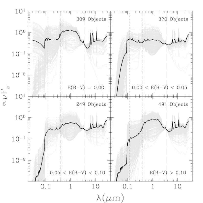
Figure 11: All best fit SEDs (gray) and their average (black) for point source AGNs with good photometric redshifts ($|z_{p}-z_{s}|<0.2$) in four ranges of the AGN reddening. The number of objects used in each case is shown in the top-right corner of each panel. All SEDs are normalized to match at 3.6$\mu$m. The vertical lines show the wavelength of Lyman-$\alpha$ (dotted), 4000Å (dot-dashed) and 3.6$\mu$m (dashed). The extreme scatter at wavelengths shorter than Ly$\alpha$ is due to large variations in IGM absorption with redshift.

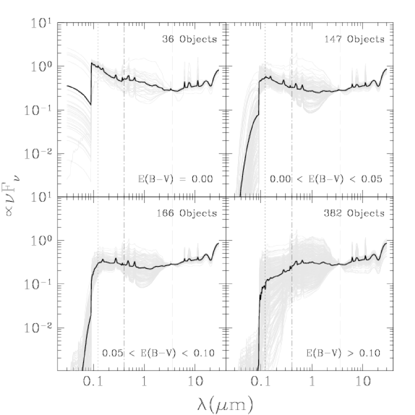
Figure 12: Same as Figure 11, but for point source AGNs with bad photometric redshifts ($|z_{p}-z_{s}|>0.5$). Note how these sources have very flat, featureless SEDs compared to those in Fig. 11. For most of these AGN, the Lyman break is not in the range of the data.

The photometric redshift accuracies for AGNs are much worse. For extended AGNs, the dispersion is 20% larger than for galaxies ($\Delta z=0.050$) and for point source AGNs it is a factor of $\sim 4.5$ worse ($\Delta z=0.18$). This lower accuracy is similar to the results of Rowan-Robinson et al. (2008) for QSOs in the SWIRE survey. The problem can be largely attributed to the lack of prominent broad-band features in the SED of AGNs as compared to galaxies. For many objects, the AGN continuum combined with that of the host produces an extremely flat SED, and for these objects the photometric redshift estimate is dominated by secondary factors like photometry errors and the galaxy luminosity prior we apply to the hosts. The latter has the effect of assigning severely underestimated redshift values to many sources, although removing it improves the median shift but worsens the accuracy. Figures 11 and 12 show the average best fit SEDs for the point source AGNs with “good” and “bad” photometric redshifts (defined by $|z_{p}-z_{s}|<0.2$ and $|z_{p}-z_{s}|>0.5$ respectively) as a function of the estimated reddening of the AGN. It is very clear that the objects with good photometric redshifts have significantly stronger host components than those with bad estimates. In particular, the objects with good redshifts appear to have a distinctive inflexion point close to 4000Å which probably constrains the photometric redshift.

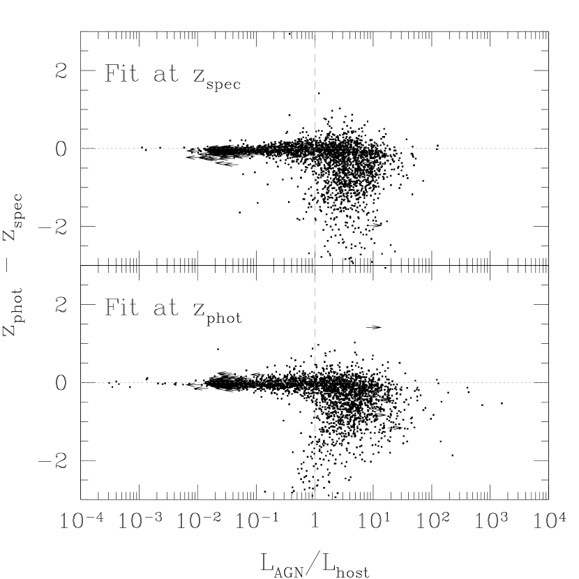
Figure 13: Difference between the photometric and spectroscopic redshift of all point source AGNs in our sample as a function of the bolometric luminosity ratio between the best fit AGN and host components. Arrows show upper or lower limits when either the AGN or the host components were not used in the best fit. When the AGN is more luminous than its host (rightward of vertical gray dashed line), the photometric redshift accuracy is poor.

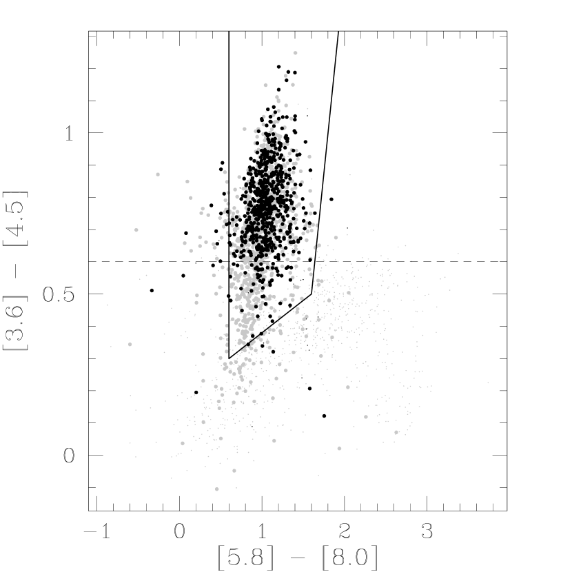
Figure 14: IRAC color-color diagram of all point source AGNs in our sample. Black points to the objects with bad photometric redshifts ($|z_{p}-z_{s}|>0.5$) while the rest are shown in gray. Large points mark objects classified by the modified SDSS pipeline to have active nuclei, while the rest correspond to the small symbols. Notice that the majority of solid circles lie at $\rm[3.6]-\rm[4.5]$ colors redder than 0.6. The solid lines mark the AGN color selection region of Stern et al., (2005).

To further explore this point, we show in Figure 13 the difference between the photometric and spectroscopic redshifts as a function of the ratio between the bolometric luminosities of the AGN and host components for all objects classified as point source AGNs. Note that we have not included the galaxy luminosity prior when fitting the SED at $z_{p}$ (although $z_{p}$ is calculated with the prior), as it is not included for the fits at $z_{s}$ to which we are comparing. Independent of whether we estimate the ratio at $z_{s}$ or $z_{p}$, the photometric redshift accuracy is markedly better when the best fit AGN component is fainter than the host component. For $L_{\rm AGN}<L_{\rm Host}$, the photometric redshift dispersion is $\Delta z=0.041$ for extended AGNs and $\Delta z=0.081$ for the point source ones, while when $L_{\rm AGN}>L_{\rm Host}$, the dispersions rise to 0.145 and 0.224 respectively. Because there is a marked dependence of the photometric redshift accuracy on the host galaxy strength relative to the AGN SED, an IRAC color dependence is also expected. Figure 14 shows the IRAC color-color diagram where the points have been color-coded according to their photometric redshift accuracy. Most of the objects with bad redshift estimates lie at colors redder than [3.6]–[4.5] = 0.6.

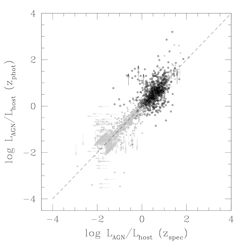
Figure 15: Comparison of the bolometric luminosity ratios between the AGN and host components for all point source AGNs (solid gray points). Points with black borders correspond to objects with bad photometric redshift determinations ($|z_{p}-z_{s}|>0.5$). When either the AGN or the host component is not detected, an arrow shows the upper/lower limit of the respective ratio. Note that the ratios are not systematically biased when the photometric redshifts are used instead of the spectroscopic ones.

From Figure 13 it is possible to see that the $L_{\rm AGN}/L_{\rm Host}$ ratio is little changed whether we use the true or photometric redshift of the source. This is more clearly shown in Figure 15 and has two interesting implications. First, since this ratio is not highly dependent on the photometric redshift, it can be used as a sign of the photo-z’s likely reliability even in the absence of spectroscopic confirmation. And second, the ability of our templates to measure $L_{\rm AGN}/L_{\rm Host}$ is not dependent on whether the true redshift of the source is known, and hence can be used to target (essentially) high Eddington ratio AGNs using purely photometric redshifts.

At the highest redshifts of our sample ($z>4$), photometric redshifts are affected by a color degeneracy between the Lyman break at high redshift and the Balmer break at low $z$, mainly caused by their lack of detection in the GALEX and Bw bands. It is clear from Figure 10 that if this degeneracy is broken, by, for example, a combination of deeper UV imaging and stronger upper bounds, the photometric redshift accuracy for these objects can be very good. If we recalculate the photometric redshifts for these objects but only allowing for $z_{p}>1$, we obtain an accuracy of $\sigma_{z}/(1+z)=0.072$. Note that this degeneracy is not related to the fact that we fixed the IGM absorption, as the accuracies for these high redshifts worsens if we allow the IGM absorption strength to vary.

We have shown the lack of accuracy in the broad-band photometric redshifts of AGNs is a product of the lack of spectral features in their SEDs. Regardless, it is important to understand if these photometric redshifts really just lack precision or truly lack accuracy. Based on the probability distribution function (PDF) of each object, we have calculated 68.3% and 95.4% errorbars on the photometric redshifts. The error bars are asymmetric and have been defined to include the given percentage of the PDF to either side of the maximum. For inactive galaxies we find that the average difference between the 1$\sigma$ (2$\sigma$) upper and lower limits of the photometric redshifts is 0.08 (0.16), while we find 0.10 (0.21) for optically extended AGNs and 0.25 (0.54) for optical point source AGNs. This shows that our photometric redshifts for AGNs lack the precision of those of inactive galaxies and extended AGNs. If we recalculate $\sigma_{z}/(1+z)$ ($\Delta z$) limited to objects where the 68.3% range of the photometric redshifts is less than 0.1, the range of the optically extended AGNs, we find 0.062 (0.036) for inactive galaxies, 0.109 (0.036) for optically extended AGNs and 0.253 (0.118) for optical point source AGNs. The lack of improvement in these statistics for the optical point source AGNs suggests that the lack of spectral features in the SED of the AGNs not only worsens the precision, but also the accuracy of the photometric redshifts.

The low accuracies of AGN photometric redshifts we have obtained at $z<4$ can be generally extrapolated to all SED fitting algorithms relying solely on broad-band data in the UV to mid-IR wavelength regime, as it is caused by the lack of strong spectral features inherent to the SEDs of AGNs and not to a method in particular. Nonetheless, other approaches that do not rely solely on broad-band SED fits have proven to be significantly more successful. In particular, the addition of narrow and medium photometric bands observations can help constrain the photometric redshifts for AGNs, as shown by Wolf et al. (2003), who obtained a dispersion of $\sigma=0.03$ for AGNs in the COMBO-17 survey, and by Salvato et al. (2009), who obtained $\sigma/(1+z)\sim 0.015$ for QSOs with $i^{*}_{AB}<24.5$ in the COSMOS field. Narrower bands significantly enhance the photometric effects of emission lines. Estimates based on neural networks can also provide accurate photometric redshifts for AGNs. In particular, Brodwin et al. (2006) used this approach to obtain redshifts for QSOs using an earlier version of the photometry used in this paper for the NDWFS Boötes field. We have compared their redshift estimates with ours for a sample of 2290 active objects with SEDs dominated by the AGN. While our SED fitting method gives $\sigma/(1+z)=0.18$, the neural network approach of Brodwin et al. (2006) has an accuracy $\sigma/(1+z)=0.13$, about 25% better.

4.3 Mid-IR AGN Selection

Mid-IR photometry has been proven to be a robust and efficient tool to select AGNs without prior information (e.g. Lacy et al., 2004; Stern et al.,, 2005; Richards et al.,, 2006), as their properties at these wavelengths are typically very different from those of stars and galaxies. Mid-IR selection methods also avoid some of the biases against extincted AGN or AGN with $z\sim 3$ found in optical surveys. In this section we use our galaxy and AGN SED templates to study the selection of active galaxies by their Spitzer IRAC colors and possible selection biases as a function of redshift and reddening of the central engine. In particular, we will focus on the selection criteria developed by Stern et al., (2005) and Lacy et al. (2004), as they are the most commonly used AGN selection methods based on IRAC colors.

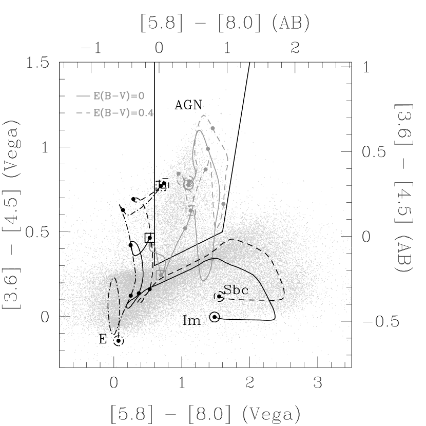
Figure 16: IRAC band color-color diagram of $I\leq 21.5$ SDWFS sources (gray dots). Overlaid are the AGN selection region of Stern et al., (2005) (solid black boundaries) and the color tracks (as a function of redshift) of our E (dot-dashed black line), Sbc (dashed black line) and Im (solid black line) galaxy SED templates, and of our AGN template for no reddening (solid gray line) and for a reddening of $E(B-V)=0.4$ (dashed gray line). For the galaxy templates, color tracks are shown for redshifts between 0–3, while for the AGN template they are shown between 0–10. Each heavy dot marks an increase of unity in redshift for the galaxies and an increase of 2 units of redshift for the AGN. For each template, the heavy dot surrounded by a circle marks $z=0$ while those surrounded by a square mark the terminal redshift ($z=3$ for galaxies and $z=10$ for the AGN).

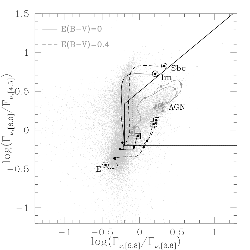
Figure 17: Same as Figure 16 but in the colors used by Lacy et al. (2004) to define their AGN selection criterion (solid black boundaries). We also shown the updated selection criteria of Lacy et al. (2007), modified to limit the problems with contamination by low redshift galaxies (dotted black selection boundaries). Line and point styles have the same definition as in Figure 16.

Figure 16 shows the mid-IR color space of the SDWFS survey (only objects with $I<21.5$ to limit the contamination by unflagged stars) along with the Stern et al., (2005) quasar selection criterion and the color tracks of our templates ($z<3$ for the galaxy templates and $z<10$ for the AGN). All low redshift galaxies have very similar [3.6]–[4.5] colors, as this is dominated by their stellar emission. However, they populate two different regions of the [5.8]–[8.0] color, where the difference is dust/PAH emission in star forming galaxies and its absence in ellipticals. As the redshift increases, the colors converge and follow very similar tracks, as the bands are redshifted into the predominantly stellar emission at wavelengths shortward of $\sim 5\mu$m. The IRAC colors of AGNs are, on the other hand, dominated by hot dust emission at low redshifts/long wavelengths, and by emission of the accretion disc at higher redshifts/short wavelengths. As a result, AGNs populate a very distinct region of the IRAC color-color space from low and intermediate redshift galaxies, and the Stern et al., (2005) or Lacy et al. (2004) selection criterion approximately delineate this region. Notice that, as shown in Figures 16 and 17, high redshift galaxies ($z\gtrsim 3$) occupy a very similar region to AGNs in the IRAC colors, and contaminate both selection criteria. Yun et al. (2008) has also shown that this is the case for submillimetre-bright galaxies at $z>2$. However, since AGNs are commonly much more luminous than galaxies, these issues are only significant for faint sources.

The Stern et al., (2005) selection criterion does a remarkably good job of separating the low and intermediate redshift galaxies from the AGN. Its only significant problems are the “blue loop” out of the region at $z\simeq 4.5$, where the H$\alpha$ line is redshifted into the [3.6] band, and the requirement that the AGN, rather than the host, dominates the mid-IR SED (Gorjian et al., 2008). A survey with mid-IR completeness problems near the $z\simeq 4.5$ loop can be easily handled by including bluer mid-IR objects that also show evidence for a Lyman limit in the optical. At $z\simeq 7$ our unreddened AGN template predicts a similar problem when H$\beta$ is redshifted into the [3.6] band, and the mid-IR colors resemble those $z\sim 1-2$ galaxies. Moderately reddened AGN stay inside the Stern et al., (2005) selection boundaries at all redshifts, as illustrated in Figure 16 for $E(B-V)=0.4$. With this amount of reddening, when $H\alpha$ is redshifted into the [3.6] channel, the colors reach the selection boundary but are always inside of it. Note, however, that there is a host dependence on the amount of reddening necessary to stay inside the selection boundaries. As shown by Hickox et al. (2007) (see also the top left panel of Fig. 6), more highly reddened objects can more easily exit the AGN selection boundaries due to host contamination, as it is harder to meet the requirement that the AGN dominates the SED.

The mid-IR AGN selection criterion defined by Lacy et al. (2004) does not suffer from the $z\sim 4.5$ incompleteness problem. However, it does suffer from large amounts of contamination by low redshift star forming galaxies. Figure 17 shows the SDWFS sources in the color space used by Lacy et al. (2004) to define their AGN selection criterion. The AGN colors stay inside the selection boundaries throughout the whole redshift range from 0–10. However, star forming galaxies characterized by the Sbc template are also contained within the selection region at $0.25\lesssim z\lesssim 1$. Note that this also means the requirement that the AGN dominates the SED is somewhat more relaxed than for the Stern et al., (2005) selection criterion. A redder $S_{5.8}/S_{3.6}$ limit would eliminate most star forming galaxies, but at the cost of introducing the bias against high redshift QSOs. Hence, the differences between the Stern et al., (2005) and Lacy et al. (2004) AGN selection criteria can be regarded as a trade-off between completeness and galaxy contamination. Figure 17 also shows an updated version of this criteria by Lacy et al. (2007), on which the vertical boundary has been shifted by 0.1. This modified boundary keeps the completeness of Lacy et al. (2004) and somewhat reduces the galaxy contamination.

Recently, Richards et al. (2009) used IRAC observations of SDSS objects to compare both of the selection criteria, and their results are in very good agreement with ours. They find that the Stern et al., (2005) selection criteria is much less contaminated by inactive galaxies in comparison to that of Lacy et al. (2004), but that the Stern et al., (2005) selection is biased against AGNs in the redshift range $3.5<z<5$. We find that this problem is restricted to a somewhat narrower redshift range. In an earlier work, Donley et al. (2008) used objects in the GOODS-S field (Giavalisco et al., 2004) to compare the reliability of these two AGN selection criteria in addition to the power-law galaxies selection method of Alonso-Herrero et al. (2006) and Donley et al. (2007). Donley et al. (2008) concludes that the Stern et al., (2005) selection diagram has more overlap with color tracks of inactive galaxies than that of Lacy et al. (2004), suggesting that AGN selection by the former is subject to more contamination. This is possibly due to including significantly fainter galaxies, but the dominant cause seems to be that their SED models exaggerate the color space populated by galaxies. As can bee seen in their Figure 6 for objects with $0.25\leq z\leq 0.75$, few non-AGN actually lie in the Stern et al., (2005) region even though the SED tracks would allow them to do so.

4.4 Colors of Galaxies and AGNs in WISE

The Wide-Field Infrared Survey Explorer (WISE; Mainzer et al., 2005) commenced an all-sky survey in the mid-IR in late 2009. The survey will be made in 4 bands with effective wavelengths of approximately 3.4, 4.6, 12 and 22$\mu$m, estimated by assuming a source with flux $F_{\nu}\propto\nu^{-1}$. The two shortest wavelength bands are similar to the [3.6] and [4.5] channels of IRAC while the longest wavelength band is similar to the MIPS 24$\mu$m channel. Following the notation we have adopted for the IRAC bands, we will refer to the WISE bands by [3.4], [4.6], [12] and [22]. The average survey depth (8 repeated observations, 5$\sigma$) will be 0.12, 0.16, 0.65 and 2.6 mJy, respectively. For comparison, the average depth (6″ apertures, 5$\sigma$) of the SDWFS survey in the two shortest wavelength IRAC bands are 5.2 and 7.2 $\mu$Jy respectively (Ashby et al., 2009), about 20 times deeper than the average WISE field.

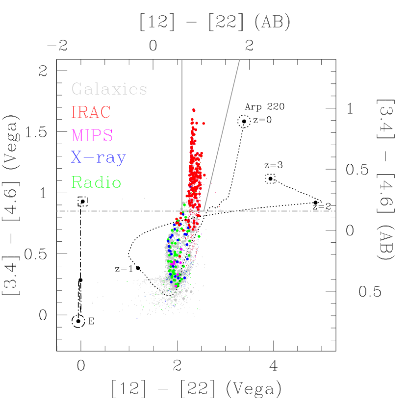
Figure 18: WISE band color-color diagram of all SDWFS sources that would be detected in the [3.3] and [4.6] bands (small dots), or in all four channels simultaneously (large dots). Each color represents objects that were targeted for spectroscopy by AGES (but not necessarily observed) as IRAC (red), MIPS (magenta), X-ray (blue) and/or radio (green) AGNs, or as non-active galaxies (gray). These are applied sequentially, so the MIPS points are only those that were not IRAC selected and so forth. The selection boundaries using all four channels (solid gray line) and just the $[3.3]-[4.6]$ color (dot-dashed gray line) are also shown. For reference, we show the color tracks of the SED of Arp 220 (dotted black line) and of our E template (dot-dashed black line) as a function of redshift. For each of the SEDs color tracks, heavy dots mark an increase in redshift of unity, while the large open circle marks $z=0$ and the large open square marks $z=3$ for Arp 220 and $z=2$ for the E template.

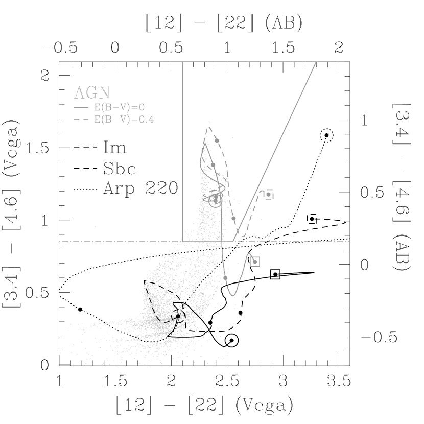
Figure 19: Color tracks of our SED templates and of the SED of Arp 220, overlaid on top of all SDWFS sources that would be detected at [3.3] and [4.6] by WISE (gray dots). The different line-styles have the same definition as in Figures 16 and 18. Note that, because of the shallow depths of the WISE mission, we only show the color tracks up to $z=2$, 6 and 3 for galaxies AGN and Arp 220 respectively. Most of the Arp 220 track extends off the red edge of the Figure (see Fig. 18 for the complete color track).

We can combine our object samples and templates to synthesize WISE observations. For this purpose we use the measured WISE filter curves, including the detector response (Wright 2009, private communication). These are shown in Figure 1. Table 2 shows the AB absolute magnitudes of our templates in the WISE bands as a function of redshift. Figure 18 shows the WISE colors as synthesized by our templates for all SDWFS sources that will be brighter than the WISE [3.4] and [4.6] magnitude limits and have $I<22.5$. Figure 19 shows the color tracks of our AGN template ($0<z<6$), our star forming galaxy templates ($0<z<2$) and the GRASIL (Silva et al., 1998) Arp 220 SED ($0<z<3)$. The latter is also shown in Figure 18 along with the color tracks of our E template ($0<z<2$). Note that the low redshift ($z\lesssim 0.5$) [12] and [22] fluxes of AGNs are not reliable because there are too few pure AGNs in our sample at these low redshifts to stably determine the AGN SED at these wavelengths. The apparent lack of pure elliptical galaxies in Figure 18 is an artifact. Tiny contributions from the star forming SED templates significantly modify the colors of such galaxies in the two longest wavelength bands, whether these contributions are real (e.g. 24$\mu$m excess red galaxies of Brand et al., 2009) or simply an artifact due to model uncertainties.

Of the 3973 sources in Figures 18 and 19, 3694 have spectroscopic redshifts and we use photo-z’s for the rest. We have eliminated all photo-z objects with fits having $\chi^{2}>50$ (63% of the photo-z sources) in order to limit contamination by stars. Since the WISE survey is significantly shallower than SDWFS, essentially all the AGNs at the WISE depths have spectroscopic redshifts and our results are little affected by any problems with their photometric redshifts. Objects targeted by AGES as AGNs are marked in Figure 18 according to the criterion by which they were selected. Objects targeted by multiple criteria are marked only by one criterion, where the priority ordering was IRAC, MIPS, X-ray and, lastly, radio selection. IRAC selected AGNs clearly populate a distinct region of the WISE color-color diagram, well separated from galaxies.

Non-IRAC targeted X-ray and radio candidates have a much larger scatter and tend to populate a region that extends between the colors of IRAC selected AGNs and normal star forming galaxies. This is explained by the requirement that IRAC selected AGN must have higher Eddington ratios, so that color is dominated by the AGN in the rest-frame mid-IR. Lower Eddington ratios have colors contaminated by the host, and hence have mid-IR colors increasingly dominated by stars and cold dust emission from star formation. X-ray sources are little affected by host contamination and so are still found when the mid-IR colors are dominated by the host (Gorjian et al., 2008), while the WSRT radio survey is deep enough to detect radio emission associated with star formation as well as AGN. Note that for $z\gtrsim 0.5$ the host contamination needed to move Type 1 AGNs out of the selection region is not just a function of its SED and the Eddington ratio of AGN, but also of reddening, as both, the [3.4] and [4.6] channels can be affected by extinction.

In an analogous way to the AGN selection region defined by Stern et al., (2005), we propose the following color-color criterion for selecting AGNs in WISE observations,

$$[12]-[22]>2.1$$ (5)

$$[3.4]-[4.6]>0.85$$ (6)

$$[3.4]-[4.6]>1.67\ ([12]-[22])-3.41,$$ (7)

as shown in Figures 18 and 19. Like the Stern et al., (2005) selection method, it will have little contamination from low and intermediate redshift galaxies. The left boundary is chosen because there do not seem to be any AGNs at redder colors either observationally or based on our templates. The other two boundaries are selected as a compromise between maximizing the number of WISE selected AGNs and limiting the contamination by intermediate redshift galaxies and ULIRGS, were we have characterized the latter by the SED of Arp 220. In particular, the rightmost boundary separates AGNs from low ($z\lesssim 0.2$) and high ($z\gtrsim 2$) redshift ULIRGs. ULIRGs are relatively rare and interesting, so the simple and deeper criterion for selecting AGNs of

$$[3.4]-[4.6]>0.85\ ,$$ (8)

(the dashed line in Figure 18) may be all that is needed. Note that all WISE selection criteria have significant problems at $z\gtrsim 3.4$, starting when H$\alpha$ emission is redshifted into the [3.4] band, analogous to our earlier discussion of the Stern et al., (2005) selection criterion. However, in this case, reddened AGN do not re-enter the selection region at higher redshifts. WISE data will need to be merged with other information to separate high redshift QSOs from lower redshift galaxies.

Inside the full selection color region described by equations (5), (6) and (7), we find 140 Boötes objects flagged as AGN by one of the methods described in §2 and that are bright enough to be detected by WISE in all of its channels. Since the full NDWFS Boötes field survey area is approximately 9 deg², scaling to a full sky survey area we predict that WISE should find $640,000$ AGNs, corresponding to a number density of 16 deg^-2, using our color selection criteria. If only the criterion of equation (8) is applied, we find 375 objects flagged as AGN and bright enough to be detected in the two shortest wavelength channels of WISE. Again scaling to the full sky area of WISE, we predict it should find $1,700,000$ AGNs corresponding to a number density of 42 deg^-2. Ashby et al. (2009) estimated a high surface density but used a bluer cut of [3.4]–[4.6] which will introduce significant contamination by ULIRGS and star forming galaxies at low and intermediate redshifts.

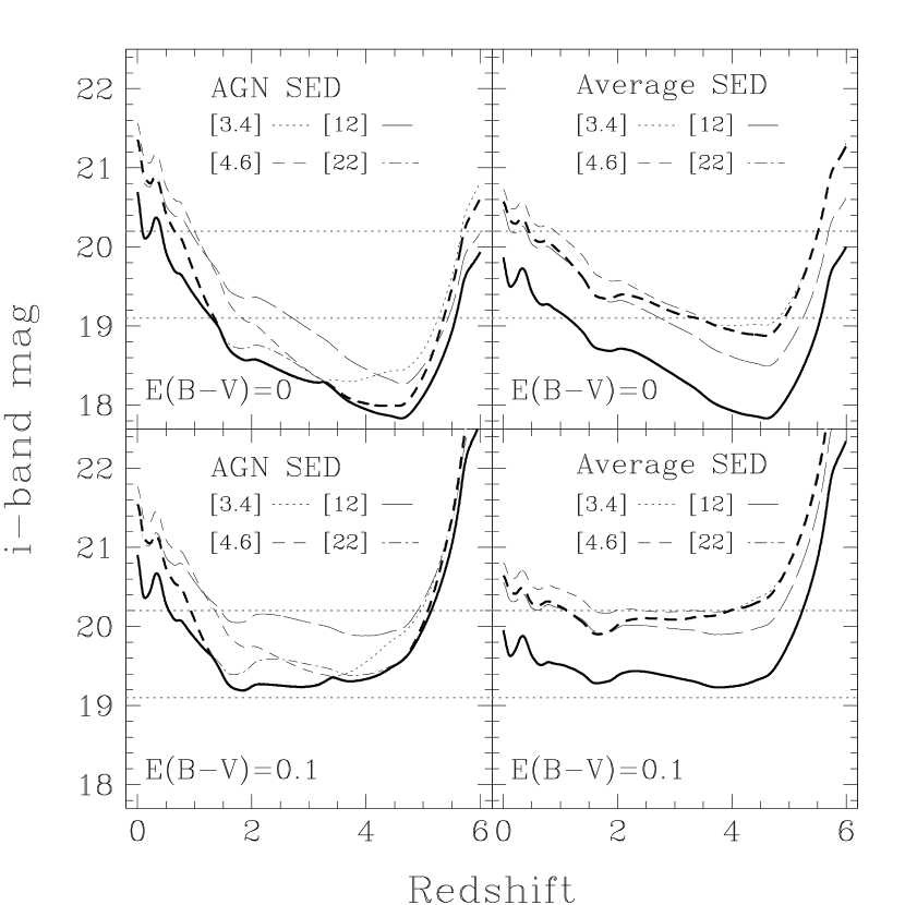
Figure 20: This Figure shows the effective $i$-band magnitude limits of the WISE survey for unreddened AGNs (top) and moderately reddened AGNs ($E(B-V)=0.1$,bottom), for pure AGN SED on the left and the average AGN + Host SEDs of IRAC-selected AGNs on the right. Each black line shows the $i$-band magnitude corresponding to the depth of each WISE band as a function of redshift. The bold solid (bold-dashed) black line shows the $i$-band magnitude limit when detection is required in all four (two shortest wavelength) WISE bands. The dotted gray lines show the SDSS limits for $z<2.3$ ($i<19.1$) and $z\leq 2.3$ ($i<20.2$).

These surface densities are higher than those of the SDSS survey, which finds 11.2 deg^-2 with $z<2.3$ and $i<19.1$ and 1.03 deg^-2 and $i<20.2$, but the differences are not a simple change in this numbers. Figure 20 shows the $i$-band magnitude limit corresponding to the WISE band detection limits for several models of AGN SEDs. For our pure AGN template without a host or extinction, the effective $i$-band depth of the WISE sources changes strongly with redshift, reaching a minimum at $z\sim 4.5$ and then rising again. The drop at low redshift is due to the v-shaped structure of the SED (see Fig. 3) - the ratio of optical to mid-IR fluxes rises with redshift until the minimum at 1$\mu$m enters the mid-IR band passes at $z\sim 4$, while at the same time the IGM absorption begins to remove optical flux. Adding a typical level of host emission markedly reduces these effects by filling in the minimum of the SED, to make the effective optical magnitude limit of WISE for the [3.4]/[4.6] bands deeper than $i=19.1$ at almost all redshifts. Adding a small amount of extinction to suppress the optical relative to the mid-IR has similar effects. Thus, the WISE sample will complement the SDSS samples.

5 Conclusions

We have created an optimized basis of low resolution SED templates for AGNs and galaxies in the wavelength range from 0.03–30$\mu$m derived from the extensive multi-wavelength observations of the NDWFS Boötes field and the AGES spectroscopic survey. This basis of templates consists of three galaxy SED templates that resemble elliptical, spiral and irregular galaxies, and an AGN SED template with variable reddening. Our model also includes IGM absorption of variable strength for high redshift sources. The templates and source codes needed to synthesize other bands and determine photo-zs are publicly available.

In this paper we have investigated three applications of our templates, namely the estimation of photometric redshifts for galaxies and AGNs, the reliability of AGN selection in the IRAC bands, and the prediction of the colors of these objects in the WISE survey as a function of redshift. In a subsequent paper (Paper II) we have used them to study the luminosity function of mid-IR selected quasars from $z=0-5.85$.

The photometric redshift accuracy of our templates for galaxies is good and comparable to other methods in the literature and to those in A08. For AGNs, however, the accuracy is much lower, in particular for those that have little contribution from the host galaxy. This is in agreement with the results of Rowan-Robinson et al. (2008) for QSOs in the SWIRE survey. The photometric redshift accuracy is highly correlated with the relative luminosities of the AGN and host components ($L_{\rm AGN}/L_{\rm Host}$), in the sense that the accuracy is lower for higher AGN fractions. In this limit, the SEDs of AGNs are flat, leaving no strong features for determining the photo-zs in broad-band photometry. When only objects where $L_{\rm AGN}<L_{\rm Host}$ are considered, the photometric redshift accuracy is comparable to that of normal galaxies. We find that the estimate of $L_{\rm AGN}/L_{\rm Host}$ is robust even when the photo-z is inaccurate.

We have also used our templates to study the color distribution of galaxies and AGNs in the IRAC bands as a function of redshift and AGN reddening, and how this affects the selection criteria of Lacy et al. (2004) and Stern et al., (2005). In particular, we have shown that the Stern et al., (2005) criterion suffers from significant incompleteness at $z\simeq 4.5$, due to the broad H$\alpha$ line being redshifted into the [3.6] band, but that it is little contaminated by low and intermediate redshift galaxies. We have also shown that the selection criterion of Lacy et al. (2004) is less subject to these sources of incompleteness but it is heavily contaminated by low redshift star-forming galaxies. Moreover, shifting the boundaries of the Lacy et al. (2004) selection region to limit the contamination by galaxies creates similar incompleteness issues to those of the Stern et al., (2005) criterion. The differences between the two selection methods can be regarded as a trade-off between completeness and galaxy contamination.

We defined two simple AGN selection criteria for the WISE satellite mission by synthesizing the WISE bands for all sources in the much deeper SDWFS survey of the Boötes field using our template models. The absolute magnitudes of our templates in the WISE bands as a function of redshift are provided in Table 2. A restrictive criteria using all 4 WISE bands would identify 140 AGN in the Boötes field, while one based only on the 2 shorter wavelength bands would identify 375. The main differences are that the more restrictive 4 filter criterion would avoid contamination by ULIRGs but is shallower because it requires detection in the less sensitive longer wavelength bands. Extrapolating from the $\sim 9~{}\rm deg^{2}$ Boötes field to the full sky, the two criteria would identify $640,000$ and $1,700,000$ AGNs respectively but largely with $z<3.4$. Additional information is needed to identify objects with $z>3.4$. These criteria should work also reasonably well in regions of high stellar density but little star formation (see e.g. Kozłowski & Kochanek, 2009, on applying the Stern et al., 2005 approach to find QSOs behind the Magellanic Clouds).

Table 1: SED Templates

$\lambda$($\mu$m)	$F_{\nu}$ (erg/s/cm2/Hz)
	AGN ($\times 10^{-11}$)	AGN 2 ($\times 10^{-14}$)	E ($\times 10^{-16}$)	Sbc ($\times 10^{-17}$)	Im ($\times 10^{-15}$)
0.0303	0.9662	5.5387	0.9659	1.9502	1.1327
0.0311	0.9838	5.7997	1.0250	2.1322	1.2553
0.0318	1.0008	6.1105	1.0829	2.2252	1.3064
0.0325	1.0153	6.4724	1.1465	2.3982	1.4211
0.0333	1.0299	6.8141	1.2075	2.5162	1.4919

Note. — Electronic table that presents the flux per unit frequency $F_{\nu}$ of our templates. The column marked as “AGN” contains our standard AGN template while that marked “AGN 2” contains the SED derived by using the Richards et al., (2006) SED as a starting point. Templates are normalized to be at a distance of 10 pc and to have an integrated luminosity between the wavelength boundaries of $10^{10}L_{\odot}$.

Table 2: SED Templates Absolute Magnitudes

$z$	Template	NUV	FUV	$B_{W}$	$B$	$V$	$R$	$I$	$z$	$J$	$H$	$Ks$	$K$	[3.6]	[4.5]	[5.8]	[8.0]	24$\mu$m	[3.4]	[4.6]	[12]	[22]	DM
0.0	1	–15.78	–15.69	–15.48	–15.36	–15.34	–15.69	–15.73	–15.32	–16.65	–17.86	–19.01	–19.10	–20.83	–21.62	–22.49	–23.53	–27.67	–17.96	–18.40	–19.70	–20.60	$\cdots$
0.0	2	–12.00	–13.63	–18.51	–18.59	–19.50	–20.13	–20.78	–20.52	–21.75	–22.50	–22.67	–22.65	–22.77	–22.64	–22.57	–22.59	–22.50	–20.06	–19.32	–17.42	–15.87	$\cdots$
0.0	3	–14.66	–15.86	–18.26	–18.28	–19.00	–19.59	–20.20	–19.94	–21.22	–22.02	–22.23	–22.22	–22.80	–22.93	–24.57	–26.06	–29.56	–20.04	–19.69	–22.04	–22.60	$\cdots$
0.0	4	–17.56	–18.05	–19.24	–19.22	–19.57	–19.88	–20.22	–19.82	–20.65	–21.12	–21.28	–21.27	–21.67	–21.68	–23.13	–24.57	–28.31	–18.95	–18.42	–20.43	–21.47	$\cdots$
0.1	1	–15.87	–15.76	–15.63	–15.50	–15.62	–15.72	–15.91	–15.38	–16.59	–17.70	–18.89	–18.98	–20.80	–21.59	–22.44	–23.52	–27.39	–17.92	–18.37	–19.64	–20.42	38.23
0.1	2	–12.02	–13.16	–17.93	–18.08	–19.36	–20.02	–20.70	–20.44	–21.80	–22.49	–22.86	–22.89	–23.01	–23.02	–22.86	–22.89	–22.82	–20.28	–19.69	–17.74	–16.19	38.23
0.1	3	–14.65	–15.66	–17.95	–18.01	–18.88	–19.50	–20.15	–19.87	–21.23	–22.01	–22.45	–22.46	–22.98	–23.11	–23.72	–26.16	–29.41	–20.20	–19.82	–22.09	–22.48	38.23
0.1	4	–17.61	–18.04	–19.10	–19.10	–19.66	–19.91	–20.28	–19.87	–20.80	–21.24	–21.50	–21.52	–21.91	–21.91	–22.37	–24.69	–28.29	–19.15	–18.61	–20.47	–21.38	38.23
0.2	1	–16.00	–15.88	–15.81	–15.67	–15.69	–15.85	–16.18	–15.49	–16.55	–17.58	–18.76	–18.86	–20.75	–21.58	–22.39	–23.52	–27.30	–17.87	–18.35	–19.61	–20.49	39.87

Note. — The electronic table supplies the absolute magnitude of each SED template (AGN: 1, E: 2, Sbc: 3 and Im: 4) for a broad range of photometric bands as a function of redshift, along with the distance modulus DM. A complete version of this table can be found in the electronic edition of the journal. Templates have been normalized to a “bolometric” luminosity of $10^{10}L_{\odot}$. The absolute magnitude we present here corresponds to the canonical definition of the absolute magnitude (as in, for example, eqn. 26 of Hogg, 1999) plus the $K$ correction term. This allows the calculation of photometric redshifts and $K$ corrections from the table. This is equivalent to Tables 3 and 4 of A08 (see their caption for details). All magnitudes are in the VEGA system except for NUV, FUV, $z$ and the WISE bands, which are in the AB system. Note that no template incorporates IGM absorption and the AGN template is unreddened. For calculating photometric redshifts and $K$-corrections allowing for variable IGM absorption and obscuration of the AGN, public numerical routines are provided on-line at http://www.astronomy.ohio-state.edu/$\sim$rjassef/lrt.

Table 3: Photometric Redshift Estimation Summary.

Sample	$\sigma_{z}/(1+z)$	$\Delta z$	68.3%	95.5%	99.7%	Median
All	0.155	0.057	0.049	0.240	0.721	-0.020
Point Source AGNs	0.261	0.184	0.174	0.544	0.777	-0.121
Extended AGNs	0.149	0.050	0.049	0.175	0.812	-0.006
Galaxies	0.128	0.041	0.042	0.127	0.429	-0.017

Note. — Summary of the photometric redshift calculations for our main catalog and each sub-sample discussed in §4.2. The table shows for each case the value of $\sigma_{z}/(1+z)$ (as defined by eqn. [4]), $\Delta z$ (the 95% clipped distribution $\sigma_{z}/(1+z)$), the ranges of $|z_{p}-z_{s}|/(1+z)$ encompassing 68.3%, 95.5% and 99.7% of the distribution and the median value of $z_{p}-z_{s}$.

Figure 4: Converged AGN SED template using the Richards et al., (2006) template as a starting point (solid line) and our standard model (dotted line). The Figure also shows the original SED template of Richards et al., (2006) (dashed line). The templates are poorly constrained near $\gtrsim 20\mu\rm m$ due to the lack of powerful low redshift quasars.Note that the bottom axis shows wavelength while the top shows frequency.

Figure 5: Average $L_{\rm AGN}/L_{\rm Host}$ obtained using the converged Richards et al., (2006) AGN SED template as a function of the ratio found using our standard AGN template. On the solid line the ratios are equal, while on the dashed lines they differ by a factor of 10. Error bars show the dispersion in each bin of $L_{\rm AGN}/L_{\rm Host}$ determined with the standard AGN template.

Figure 9: Comparison of photometric and spectroscopic redshifts for all the galaxies in our sample (right) and for the 95% with the most accurate redshift estimates (left). For a given value of the photometric redshift, we show the median spectroscopic redshift of a galaxy with that $z_{p}$ estimate (dotted line), and the 68.3% (solid line) and 95.4% (dashed line) range of the spectroscopic redshift distribution. We only show $z_{p}$ values for which there were enough objects to determine the 68.3% and 95.4% limits on both sides of the median.

Figure 10: Comparison of photometric and spectroscopic redshifts for the extended (top) and point source AGNs (bottom) in our sample considering all (right) and the 95% with the most accurate redshift estimates (left). Different line styles have the same definition as in Figure 9. The open circles show individual objects with either $z_{s}>4$ or $z_{p}>4$.

References

- Alonso-Herrero et al. (2006) Alonso-Herrero, A., et al. 2006, ApJ, 640, 167
- Ashby et al. (2009) Ashby, M. L. N., et al. 2009, ApJ, 701, 428
- Assef et al., (2008) Assef, R.J., Kochanek, C.S., Brodwin, M., Brown, M. J. I., Caldwell, N., Cool, R. J., Eisenhardt, P., Eisenstein, D., Gonzalez, A. H., Jannuzi, B. T., Jones, C., McKenzie, E., Murray, S. S., Stern, D. 2008, ApJ, 676, 286
- Assef et al., (2009) Assef et al. 2009 ApJ, in prep. (Paper II)
- Atlee et al. (2009) Atlee, D. W., Assef, R. J., & Kochanek, C. S. 2009, ApJ, 694, 1539
- Brand et al. (2009) Brand, K., et al. 2009, ApJ, 693, 340
- Becker et al., (1995) Becker, R.H., White R.L. & Helfand, D.J., 1995, AJ, 450, 559
- Brodwin et al. (2006) Brodwin, M., et al. 2006, ApJ, 651, 791
- Bruzual & Charlot, (2003) Bruzual, G. & Charlot, S. 2003, MNRAS, 344, 1000
- Budavári et al. (2001) Budavári, T., et al. 2001, AJ, 122, 1163
- Cardelli et al. (1989) Cardelli, J. A., Clayton, G. C., & Mathis, J. S. 1989, ApJ, 345, 245
- Coleman, Wu & Weedman, (1980) Coleman, G.D., Wu, C.-C. & Weedman, D.W. 1980, ApJS, 43, 393
- Condon et al., (1998) Condon, J.J. et al. 1998, AJ, 115, 1693
- Conroy et al. (2009) Conroy, C., Gunn, J. E., & White, M. 2009, ApJ, 699, 486
- Cool (2007) Cool, R. J. 2007, ApJS, 169, 21
- The Dark Energy Survey Collaboration (2005) The Dark Energy Survey Collaboration 2005, arXiv:astro-ph/0510346
- Devriendt, Guiderdoni & Sadat, (1999) Devriendt, J.E.G., Guiderdoni, B. & Sadat, R. 1999, A&A, 350, 381
- Dey et al. (2005) Dey, A. et al. 2005, submitted
- de Vries et al., (2002) de Vries, W.H. et al. 2002, AJ, 123, 1784
- Donley et al. (2008) Donley, J. L., Rieke, G. H., Pérez-González, P. G., & Barro, G. 2008, ApJ, 687, 111
- Donley et al. (2007) Donley, J. L., Rieke, G. H., Pérez-González, P. G., Rigby, J. R., & Alonso-Herrero, A. 2007, ApJ, 660, 167
- Eisenhardt et al. (2004) Eisenhardt, P. R., et al. 2004, ApJS, 154, 48
- Eldridge & Stanway (2009) Eldridge, J. J., & Stanway, E. R. 2009, MNRAS, in press. (arXiv:0908.1386)
- Elston et al., (2006) Elston, R.J., Gonzalez, A. H. et al. 2006, ApJ, 639, 816
- Elvis et al. (1994) Elvis, M., et al. 1994, ApJS, 95, 1
- Fabricant et al., (2005) Fabricant, D. et al. 2005, PASP, 117, 1411
- Fan et al., (2006) Fan, X. et al. 2006, AJ, 132, 117
- Fioc & Rocca-Volmerange (1997) Fioc, M., & Rocca-Volmerange, B. 1997, A&A, 326, 950
- Giavalisco et al. (2004) Giavalisco, M., et al. 2004, ApJ, 600, L93
- Gordon & Clayton (1998) Gordon, K. D., & Clayton, G. C. 1998, ApJ, 500, 816
- Gorjian et al. (2008) Gorjian, V., et al. 2008, ApJ, 679, 1040
- Hickox et al. (2009) Hickox, R. C., et al. 2009, ApJ, 696, 891
- Hickox et al. (2007) Hickox, R. C., et al. 2007, ApJ, 671, 1365
- Hogg (1999) Hogg, D. W. 1999, arXiv:astro-ph/9905116
- Jannuzi & Dey (1999) Jannuzi, B. T., & Dey, A. 1999, Photometric Redshifts and the Detection of High Redshift Galaxies, 191, 111
- Jannuzi et al., (2005) Jannuzi, B.T. et al. 2005, submitted.
- Kaiser (2004) Kaiser, N. 2004, Proc. SPIE, 5489, 11
- Kauffmann et al. (2008) Kauffmann, G., Heckman, T. M., & Best, P. N. 2008, MNRAS, 384, 953
- Kinney et al. (1996) Kinney, A. L., Calzetti, D., Bohlin, R. C., McQuade, K., Storchi-Bergmann, T., & Schmitt, H. R. 1996, ApJ, 467, 38
- (40) Kochanek, C.S. et al. in preparation
- Kozłowski & Kochanek (2009) Kozłowski, S., & Kochanek, C. S. 2009, ApJ, 701, 508
- Lacy et al. (2007) Lacy, M., Petric, A. O., Sajina, A., Canalizo, G., Storrie-Lombardi, L. J., Armus, L., Fadda, D., & Marleau, F. R. 2007, AJ, 133, 186
- Lacy et al. (2004) Lacy, M., et al. 2004, ApJS, 154, 166
- Lawson & Hanson, (1974) Lawson, C.L. & Hanson, R.J. 1974, Solving Least Squares Problems, PrenticeHall.
- Lawrence et al. (2007) Lawrence, A., et al. 2007, MNRAS, 379, 1599
- Leitherer et al. (1999) Leitherer, C., et al. 1999, ApJS, 123, 3
- Lin et al., (1996) Lin, H., Kirshner, R.P., Shectman, S.A., Landy, S.D., Oemler, A., Tucker, D.L. & Schechter, P. L. 1996, ApJ, 464, 60
- Mainzer et al. (2005) Mainzer, A. K., Eisenhardt, P., Wright, E. L., Liu, F.-C., Irace, W., Heinrichsen, I., Cutri, R., & Duval, V. 2005, Proc. SPIE, 5899, 262
- Martin et al., (2005) Martin, D.C. et al. 2005, ApJ, 619L, 1
- Morrissey et al. (2007) Morrissey, P., et al. 2007, ApJS, 173, 682
- Moustakas et al. (2009) Moustakas et al. 2009, in prep.
- Murray et al., (2005) Murray, S.S. et al. 2005, ApJS, 161, 1
- Rengelink et al., (1997) Rengelink, R.B. et al. 1997, A&A, 124, 259
- Richards et al. (2009) Richards, G. T., et al. 2009, AJ, 137, 3884
- Richards et al., (2006) Richards, G.T. et al. 2006, ApJS, 166, 470
- Ross et al. (2009) Ross, N. R., Assef, R. J., Kochanek, C. S., Falco, E., & Poindexter, S. D. 2009, ApJ, 702, 472
- Rowan-Robinson et al. (2008) Rowan-Robinson, M., et al. 2008, MNRAS, 386, 697
- Salvato et al. (2009) Salvato, M., et al. 2009, ApJ, 690, 1250
- Silva et al. (1998) Silva, L., Granato, G. L., Bressan, A., & Danese, L. 1998, ApJ, 509, 103
- Stengler-Larrea et al., (1995) Stengler-Larrea, E.A. et al. 1995, ApJ, 444, 64
- Stern et al., (2005) Stern, D. et al. 2005, ApJ, 631, 163
- Stern et al. (2002) Stern, D., et al. 2002, AJ, 123, 2223
- Strateva et al. (2005) Strateva, I. V., Brandt, W. N., Schneider, D. P., Vanden Berk, D. G., & Vignali, C. 2005, AJ, 130, 387
- Tananbaum et al. (1979) Tananbaum, H., et al. 1979, ApJ, 234, L9
- Tyson (2002) Tyson, J. A. 2002, Proc. SPIE, 4836, 10
- Yip et al. (2004) Yip, C. W., et al. 2004, AJ, 128, 2603
- York et al. (2006) York, D. G., et al. 2006, MNRAS, 367, 945
- Weedman et al., (2006) Weedman, D.W. et al. 2006, ApJ, 651, 101
- Wolf et al. (2003) Wolf, C., Wisotzki, L., Borch, A., Dye, S., Kleinheinrich, M., & Meisenheimer, K. 2003, A&A, 408, 499
- Yun et al. (2008) Yun, M. S., et al. 2008, MNRAS, 389, 333