Clock shifts of optical transitions in ultracold atomic gases

Abstract

We calculate the shift, due to interatomic interactions, of an optical transition in an atomic Fermi gas trapped in an optical lattice, as in recent experiments of Campbell et al., Science 324, 360 (2009). Using a pseudospin formalism to describe the density matrix of the internal two states of the optical transition, we derive a Bloch equation which incorporates both the spatial inhomogeneity of the probe laser field and the interatomic interactions. Expressions are given for the frequency shift as a function of the pulse duration, detuning of the probe laser, and the spatial dependence of the electric field of the probe beam. In the low temperature semiclassical regime, we find that the magnitude of the shift is proportional to the temperature.

In the continuing quest to develop improved atomic clocks, attention has turned to fermionic atoms because shifts of transition frequencies due to interatomic interactions (so-called clock shifts) are expected to be strongly suppressed in gases of identical fermions due to the Pauli exclusion principle. It came as a surprise that nonzero interaction shifts were observed in a recent experiment on the ¹S₀–³P₀ optical transition for ⁸⁷Sr atoms trapped in an optical lattice campbell ; ye , since for a gas of fermions it has been shown theoretically that for a homogeneous probe field there should be no frequency shift su2 . Thus inhomogeneity is indispensable for observing nonzero frequency shifts in identical fermion samples. The authors of Ref. campbell attributed the shifts to the combined influence of the spatial inhomogeneity of the probe laser field and the interatomic interaction. The same underlying physical mechanism gives rise to the Leggett-Rice effect in spin transport in liquid ³He leggett , and spin segregation in ultracold bosons cornell and fermions thomas .

In this paper, we introduce pseudospin operators to describe atomic correlations within each motional states of the atoms and derive a Bloch equation that describes the evolution of the pseudospin under the combined effect of an external probe laser field and interatomic interactions and derive expressions for the frequency shifts to be expected under the experimental conditions of Ref. campbell . Since this work was largely completed, we became aware of Refs.  gibble ; rey in which, for a particular form of the inhomogeneity of the probe field, the problem is approached using the wave function of the state.

Basic formalism. In the experiment, atoms of ⁸⁷Sr, a fermionic isotope, were initially prepared in one hyperfine state of the ³P₀ excited-state manifold (denoted by $e$) and transferred to a hyperfine state of the ¹S₀ ground-state manifold (denoted by $g$) by application of a probe laser field campbell . In the absence of the laser field, the system is described by the Hamiltonian

$$H= \int d^{3}r\sum_{\alpha=e,\,g}\psi_{\alpha}^{\dagger}(\mathbf{r})\left[-\frac{\nabla^{2}}{2m}+E_{\alpha}+V(\mathbf{r})\right]\psi_{\alpha}(\mathbf{r})$$

$$+g\int d^{3}r\psi_{e}^{\dagger}(\mathbf{r})\psi_{g}^{\dagger}(\mathbf{r})\psi_{g}(\mathbf{r})\psi_{e}(\mathbf{r}),$$ (1)

where the $\psi_{\alpha}$ are annihilation operators for atoms in the internal states $|\alpha\rangle$ and $E_{\alpha}$ are the internal energies. The effective low energy interaction coupling is given by $g=4\pi a_{s}/m$ ($\hbar=1$) where $a_{s}$ is the s-wave scattering length for collisions between a ground state atom and an excited state one. The external dipole optical potential $V(\mathbf{r})$ is a superposition of a deep one-dimensional optical lattice potential aligned along the $z$ direction for which the frequency of oscillations about the minima of the potential is $\omega_{\rm lattice}\approx 80$ kHz, and a harmonic potential with $\omega_{\perp}=\omega_{x}=\omega_{y}\approx 450$ Hz and $\omega_{z}\ll 80$ kHz. (The potential $V(\mathbf{r})$ is the same for the two atomic states since the wavelength of the optical lattice is chosen to be $\lambda_{\rm lattice}\approx 813.429$ nm, the magic wavelength at which the electric polarizabilities are the same for the ground and the excited states.) Atoms are thereby confined to a number of pancake-shaped regions extended in the $x$- and $y$-directions and centered on the $z$-axis, and are essentially limited to the ground state for motion in the $z$-direction under experimental conditions.

It is convenient to introduce the pseudospin density operators $\hat{\bf S}(\mathbf{r})=[\psi^{\dagger}_{e}(\mathbf{r}),\psi^{\dagger}_{g}(\mathbf{r})]{\boldsymbol{\sigma}}[\psi_{e}(\mathbf{r}),\psi_{g}(\mathbf{r})]^{T}/2$, where $\boldsymbol{\sigma}$ are the Pauli matrices. The coupling between the probe laser field $\mathbf{E}(\mathbf{r},t)$ and the atoms is due to dipole transitions between the two states, and can be described by the Hamiltonian

$$H_{\rm probe} =-\int d^{3}r\left(\langle e|\mathbf{d}\cdot{\bf E}(\mathbf{r},t)|g\rangle\,\psi_{e}^{\dagger}(\mathbf{r})\psi_{g}(\mathbf{r})+{\rm h.c.}\right)$$

$$=-\int d^{3}r\left({\cal B}_{x}(\mathbf{r},t){\hat{S}}_{x}(\mathbf{r})+{\cal B}_{y}(\mathbf{r},t){\hat{S}}_{y}(\mathbf{r})\right)$$ (2)

where ${\cal B}_{x}(\mathbf{r},t)=\langle e|\mathbf{d}\cdot\mathbf{E}(\mathbf{r},t)|g\rangle+\langle g|\mathbf{d}\cdot\mathbf{E}(\mathbf{r},t)|e\rangle$ and ${\cal B}_{y}(\mathbf{r},t)=i(\langle e|\mathbf{d}\cdot\mathbf{E}(\mathbf{r},t)|g\rangle-\langle g|\mathbf{d}\cdot\mathbf{E}(\mathbf{r},t)|e\rangle)$ are the components of the “pseudomagnetic field” Directions , and $\mathbf{d}$ is the electric dipole moment. Note that Refs. gibble ; rey assume only $\mathcal{B}_{x}(\mathbf{r},t)$ nonzero. However, both $\mathcal{B}_{x}(\mathbf{r},t)$ and $\mathcal{B}_{y}(\mathbf{r},t)$ depend on the details of the probe laser field and are generally not zero.

Bloch equation. We study the coherent evolution of the system governed by $H+H_{\rm probe}$ through the Bloch equations for the pseudospin operators. We expand the field operators $\psi_{\alpha}(\mathbf{r})=\sum_{i}a_{\alpha i}\phi_{i}(\mathbf{r})$, where $\phi_{i}(\mathbf{r})$ are the free particle eigenstates for $H$ with $g=0$, and $a_{\alpha i}$ are the corresponding annihilation operators. In the frame co-rotating with the probe laser, we derive

$$\frac{d}{dt}\mathbf{S}_{i}=\mathbf{\Omega}_{i}\times\mathbf{S}_{i}+2\sum_{j}g_{ij}\mathbf{S}_{i}\times\mathbf{S}_{j},$$ (3)

where $\mathbf{S}_{i}=\langle[a^{\dagger}_{ei},a^{\dagger}_{gi}]\boldsymbol{\sigma}[a_{ei},a_{gi}]^{T}\rangle/2$ and $g_{ij}=g\int d^{3}r|\phi_{i}(\mathbf{r})\phi_{j}(\mathbf{r})|^{2}$. Thus the expectation value of the total pseudospin is given by $\mathbf{S}=\sum_{i}\mathbf{S}_{i}$ with $\langle\dots\rangle$ denoting the trace with the density matrix. The probe laser field has a generic form $\mathbf{E}(\mathbf{r},t)=\mathbf{E}_{-}(\mathbf{r})\exp(-i\omega_{L}t)+\mathbf{E}^{*}_{-}(\mathbf{r})\exp(i\omega_{L}t)$ with $\omega_{L}$ the laser frequency. The driving fields $\mathbf{\Omega}_{i}=(\Omega_{ix},\Omega_{iy},\Omega_{iz})$ have components $\Omega_{ix}=\Omega_{i-}+{\rm c.c.}$, $\Omega_{iy}=i(\Omega_{i-}-{\rm c.c.})$ and $\Omega_{iz}=\Delta$, where $\Omega_{i-}=-\int d^{3}r\,|\phi_{i}(\mathbf{r})|^{2}\langle e|\mathbf{d}\cdot\mathbf{E}_{-}(\mathbf{r})|g\rangle$ and $\Delta=E_{e}-E_{g}-\omega_{L}$ is the detuning. Equation (3) is valid in the weak interaction limit, $g\to 0$, and the Lamb-Dicke regime where the recoil of the atoms due to the scattering with the probe laser is negligible and it shows that the magnitude of the pseudospin $S_{i}$ remains unaltered.

At this stage, the joint effect of the spatial inhomogeneity of $\mathbf{E}(\mathbf{r},t)$ and the interaction is manifest in Eq. (3): if all pseudospins $\mathbf{S}_{i}$ initially point towards the north pole of the Bloch sphere (as in Ref. campbell ), corresponding to all atoms being in the excited state, the first term causes the pseudospins of states with different $\mathbf{\Omega}_{i}$ to precess by different amounts, and then the interatomic interaction term no longer vanishes.

We convert Eq. (3) into an integral equation,

$$\mathbf{S}_{i}(t)= \mathbf{G}_{i}(t)\mathbf{S}_{i}(0)$$

$$+2\sum_{j}g_{ij}\int^{t}_{0}dt^{\prime}\;\mathbf{G}_{i}(t-t^{\prime})\mathbf{S}_{i}(t^{\prime})\times\mathbf{S}_{j}(t^{\prime}),$$ (4)

where $\mathbf{S}_{i}(0)$ are the initial values of the pseudospins. In the Cartesian basis ($x,y,z$), the Green’s function satisfies the equation

$$\left(\frac{d}{dt}-\mathbf{Q}\right)\mathbf{G}(t)=\delta(t)$$ (5)

with

$$\mathbf{Q}=\Omega\left[\begin{array}[]{ccc}0&-\cos\theta&\sin\theta\sin\phi\\ \cos\theta&0&-\sin\theta\cos\phi\\ -\sin\theta\sin\phi&\sin\theta\cos\phi&0\end{array}\right],$$ (9)

where $\Omega_{x}=\Omega\sin\theta\cos\phi$, $\Omega_{y}=\Omega\sin\theta\sin\phi$, $\Omega_{z}=\Omega\cos\theta$ and $\Omega=\sqrt{\Omega_{x}^{2}+\Omega_{y}^{2}+\Omega_{z}^{2}}$. The matrix $\mathbf{Q}$ can be diagonalized by the matrix $\mathbf{A}=(v_{1},v_{2},v_{3})$ where the vectors are given by $v_{1}^{T}=(\sin\theta\cos\phi,\sin\theta\sin\phi,\cos\theta)$, $v_{2}^{T}=(\cos\theta\cos\phi+i\sin\phi,\cos\theta\sin\phi-i\cos\phi,-\sin\theta)/\sqrt{2}$ and $v_{3}^{T}=(\cos\theta\cos\phi-i\sin\phi,\cos\theta\sin\phi+i\cos\phi,-\sin\theta)/\sqrt{2}$. Thus

$$\mathbf{G}(t)=\theta(t)\mathbf{A}\begin{bmatrix}1&0&0\\ 0&e^{i\Omega t}&0\\ 0&0&e^{-i\Omega t}\end{bmatrix}\mathbf{A}^{\dagger}.$$ (10)

From Eq. (4), the deviation of the total pseudospin $\mathbf{S}$ from its value without interaction, $\mathbf{S}^{0}(t)=\sum_{i}\mathbf{G}_{i}(t)\mathbf{S}^{0}_{i}(0)$, is given by

$$\delta\mathbf{S}(t)$$

$$=\sum_{i,j}g_{ij}\int^{t}_{0}dt^{\prime}\left[\mathbf{G}_{i}(t-t^{\prime})-\mathbf{G}_{j}(t-t^{\prime})\right]\left[\mathbf{S}_{i}(t^{\prime})\times\mathbf{S}_{j}(t^{\prime})\right],$$ (11)

where the subscript $i$ of $\mathbf{G}$ indicates $\mathbf{\Omega}=\mathbf{\Omega}_{i}$. Equation (11) shows that the change in the pseudospin is zero if $\mathbf{\Omega}_{i}$ is independent of $i$.

Frequency shift. In the experiments the frequencies $\delta\mathbf{\Omega}_{ij}=(\mathbf{\Omega}_{i}-\mathbf{\Omega}_{j})/2$ and $g_{ij}$ are small compared with the average $\mathbf{\Omega}_{i}$ and therefore we may treat them perturbatively. For the interatomic interaction this means that the change in the total pseudospin is a sum over contributions from independent pairs of motional states, and therefore we may consider just two motional states (which we shall denote by 1 and 2), and then sum over all possible pairs at the end. From Eq. (3), the total pseudospin of the pair of states $\mathbf{S}_{+}=\mathbf{S}_{1}+\mathbf{S}_{2}$ and the difference $\mathbf{S}_{-}=\mathbf{S}_{1}-\mathbf{S}_{2}$ satisfy the equations

$$\frac{d}{dt}\mathbf{S}_{+}= \mathbf{\Omega}\times\mathbf{S}_{+}+\delta\mathbf{\Omega}\times\mathbf{S}_{-}$$ (12)

$$\frac{d}{dt}\mathbf{S}_{-}= \mathbf{\Omega}\times\mathbf{S}_{-}+\delta\mathbf{\Omega}\times\mathbf{S}_{+}-2g_{12}\mathbf{S}_{+}\times\mathbf{S}_{-},$$ (13)

with $\mathbf{\Omega}=(\mathbf{\Omega}_{1}+\mathbf{\Omega}_{2})/2$ and $\delta\mathbf{\Omega}=(\mathbf{\Omega}_{1}-\mathbf{\Omega}_{2})/2$. Note the interaction does not appear in the equation for $\mathbf{S}_{+}$ explicitly. This is consistent with the argument based on the SU(2) symmetry of the interaction su2 : if $\delta\mathbf{\Omega}=0$, the dynamics of $\mathbf{S}_{+}$ is only governed by $\mathbf{\Omega}$ and no interaction effects can show up. The physical mechanism for creating a frequency shift due to interatomic interactions is as follows. Initially all pseudospins are aligned in the same direction, and therefore $\mathbf{S}_{+}\times\mathbf{S}_{-}$ is zero and the interaction has no effect. However, according to Eq. (13) the field inhomogeneity creates a component of $\mathbf{S}_{-}$ perpendicular to $\mathbf{S}_{+}$, and therefore the interactions can have an effect. Subsequently, according to Eq. (12) this results in a change in $\mathbf{S}_{+}$. Consequently, the leading contribution to the shift is proportional to $g(\delta\Omega)^{2}$.

For the initial conditions of interest, $\mathbf{S}_{1}(0)=S_{1}(0)\mathbf{e}_{z}$ and $\mathbf{S}_{2}(0)=S_{2}(0)\mathbf{e}_{z}$, where $S_{i}(0)=f_{i}/2$ and $f_{i}$ is the initial distribution function. Solving for the change of $\mathbf{S}_{+}(t)$ due to the interaction to second order in $\delta\mathbf{\Omega}$ and first order in $g_{12}$ by iterating integral equations similar to Eq. (4), we obtain

$$\delta\mathbf{S}_{+}(t)$$

$$= 2\int_{0}^{t}dt^{\prime}\int_{0}^{t^{\prime}}dt^{\prime\prime}\int_{0}^{t^{\prime\prime}}dt^{\prime\prime\prime}\mathbf{G}(t-t^{\prime})\delta\mathbf{\Omega}\times\mathbf{G}(t^{\prime}-t^{\prime\prime})$$

$$g_{12}\Big{\{}\big{[}\mathbf{G}(t^{\prime\prime})\mathbf{S}_{-}(0)\big{]}\times\big{[}\mathbf{G}(t^{\prime\prime}-t^{\prime\prime\prime})\delta\mathbf{\Omega}\times\mathbf{G}(t^{\prime\prime\prime})\mathbf{S}_{-}(0)\big{]}$$

$$+\big{[}\mathbf{G}(t^{\prime\prime}-t^{\prime\prime\prime})\delta\mathbf{\Omega}\times\mathbf{G}(t^{\prime\prime\prime})\mathbf{S}_{+}(0)\big{]}\times\big{[}\mathbf{G}(t^{\prime\prime})\mathbf{S}_{+}(0)\big{]}\Big{\}}.$$ (14)

The processes corresponding to this equation are that at time $t^{\prime\prime\prime}$ the diffence in precession frequencies gives rise to a difference in orientations of the two pseudospins, then the interatomic interaction acts at time $t^{\prime\prime}$ and finally the difference of precession frequencies leads to a change in the total pseudospin of the pair of states. After simplification Eq. (14) becomes

$$\delta\mathbf{S}_{+}(t)$$

$$= -8g_{12}S_{1}(0)S_{2}(0)\int_{0}^{t}dt^{\prime}\int_{0}^{t^{\prime}}dt^{\prime\prime}\int_{0}^{t^{\prime\prime}}dt^{\prime\prime\prime}\mathbf{G}(t-t^{\prime})\delta\mathbf{\Omega}$$

$$\times\mathbf{G}(t^{\prime}-t^{\prime\prime})\Big{\{}\mathbf{G}(t^{\prime\prime})\mathbf{e}_{z}\times\big{[}\mathbf{G}(t^{\prime\prime}-t^{\prime\prime\prime})\delta\mathbf{\Omega}\times\mathbf{G}(t^{\prime\prime\prime})\mathbf{e}_{z}\big{]}\Big{\}}.$$ (15)

The quantity measured in experiment is the population of atoms in the ground state, ${\rm P}_{g}=N/2-\sum_{i}S_{iz}$, where $N$ is the total number of atoms. On summing Eq. (15) over all pairs of motional states one finds

$$\delta{\rm P}_{g}(t)=C_{1}\Xi_{1}+C_{3}\Xi_{3}+C_{3}\Xi_{3},$$ (16)

where

$$\Xi_{1}= \sum_{i,j}\frac{4g_{ij}S_{i}(0)S_{j}(0)}{\Omega_{xy}^{3}}(\delta\mathbf{\Omega}_{ij\parallel})^{2}$$ (17)

$$\Xi_{2}= \sum_{i,j}\frac{4g_{ij}S_{i}(0)S_{j}(0)}{\Omega_{xy}^{3}}(\delta\mathbf{\Omega}_{ij\perp})^{2}$$ (18)

$$\Xi_{3}= \sum_{i,j}\frac{4g_{ij}S_{i}(0)S_{j}(0)}{\Omega_{xy}^{3}}\mathbf{e}_{z}\cdot(\delta\mathbf{\Omega}_{ij\parallel}\times\delta\mathbf{\Omega}_{ij\perp})$$ (19)

and

$$C_{1}= \frac{\delta}{6\left(1+\delta^{2}\right)^{4}}\left\{3\left(2+\delta^{2}\right)\sin^{2}\left(\tau\sqrt{1+\delta^{2}}\right)\right.$$

$$-3\left[\tau^{2}+\left(3\tau^{2}-4\right)\delta^{2}+2\left(2+\tau^{2}\right)\delta^{4}\right]$$

$$\times\cos\left(\tau\sqrt{1+\delta^{2}}\right)+3\left[4\delta^{4}-4\delta^{2}-\tau^{2}\left(1+\delta^{2}\right)\right]$$

$$+\tau\sqrt{1+\delta^{2}}\left[\tau^{2}+\left(\tau^{2}+9\right)\delta^{2}-6\delta^{4}\right]$$

$$\left.\times\sin\left(\tau\sqrt{1+\delta^{2}}\right)\right\},$$ (20)

$$C_{2}= \frac{\delta}{2\left(1+\delta^{2}\right)^{7/2}}\left\{4\delta^{2}\sqrt{1+\delta^{2}}-4\delta^{2}\sqrt{1+\delta^{2}}\right.$$

$$\left.\times\cos\left(\tau\sqrt{1+\delta^{2}}\right)-\sqrt{1+\delta^{2}}\sin^{2}\left(\tau\sqrt{1+\delta^{2}}\right)\right.$$

$$\left.-\tau\left(-1+\delta^{2}+2\delta^{4}\right)\sin\left(\tau\sqrt{1+\delta^{2}}\right)\right\},$$ (21)

$$C_{3}= \frac{2\sin^{2}\left(\tau\sqrt{1+\delta^{2}}/2\right)}{\left(1+\delta^{2}\right)^{5/2}}$$

$$\times\left\{-\tau\sqrt{1+\delta^{2}}+\sin\left(\tau\sqrt{1+\delta^{2}}\right)\right\},$$ (22)

with $\delta=\Delta/\Omega_{xy}$, $\tau=\Omega_{xy}t$, $\mathbf{\Omega}_{xy}=\overline{\mathbf{\Omega}}_{i}-\Delta{\mathbf{e}}_{z}$, $\delta\mathbf{\Omega}_{ij\parallel}=(\delta\mathbf{\Omega}_{ij}\cdot\mathbf{\Omega}_{xy})\mathbf{\Omega}_{xy}/\Omega_{xy}^{2}$, and $\delta\mathbf{\Omega}_{ij\perp}=\delta\mathbf{\Omega}_{ij}-\delta\mathbf{\Omega}_{ij\parallel}$. Here the bar denotes an average over motional states.

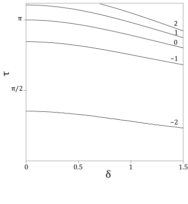
Figure 1: Contour plot of the frequency shift $\delta\omega$, in units of $(2N/\Omega_{xy}^{2})\,\overline{g_{ij}(\mathbf{\Omega}_{i}-\mathbf{\Omega}_{j})^{2}}$ as a function of dimensionless detuning, $\delta=\Delta/\Omega_{xy}$ and dimensionless pulse duration, $\tau=\Omega_{xy}t_{p}$.

Experimentally, the pulse duration $t_{p}$ is fixed and pairs of detunings $\Delta_{1}$ and $\Delta_{2}$ which render the same population ${\rm P}_{g}$ in the ground state at the end of the pulse, i.e., $S_{z}(t_{p},\Delta_{1})=S_{z}(t_{p},\Delta_{2})$, are measured. The clock shift is defined as $\delta\omega=(\Delta_{1}+\Delta_{2})/2$. The reason why this method can detect the effects of interatomic interactions lies in the symmetry of the Bloch equation (3). For simplicity, let us assume $\Omega_{iy}=0$. Without interactions, Eq. (3) is invariant under the transformation $\{\Delta,S_{ix},S_{iy},S_{iz}\}\to\{-\Delta,-S_{ix},S_{iy},S_{iz}\}$, which implies $\Delta_{1}=-\Delta_{2}$ and $\delta\omega=0$. When $g\neq 0$, Eq. (3) becomes invariant under the transformation $\{\Delta,g,S_{ix},S_{iy},S_{iz}\}\to\{-\Delta,-g,-S_{ix},S_{iy},S_{iz}\}$, which indicates $\delta\omega\neq 0$ if $\Omega_{i}$ are different. To order $g(\delta\Omega)^{2}$, from Eq. (16), we have

$$\delta\omega=\frac{2\delta S_{z}(t_{p},\Delta)}{dS_{z}^{0}(t_{p},\Delta)/d\Delta}.$$ (23)

Field inhomogeneity. To compare our results with experiment we need to take into account the form of the probe laser field, which is a linearly polarized Gaussian beam. With the assumption that the axis of symmetry of the laser field coincides with that of the optical trap, the electric field vector is given by

$$\mathbf{E}_{-}(\mathbf{r})= E_{0}\mathbf{e}_{x}\frac{w(0)}{w(z)}\exp\left(-\frac{x^{2}+y^{2}}{w^{2}(z)}\right)$$

$$\times\exp\left(i\frac{2\pi}{\lambda_{L}}z+i\frac{\pi(x^{2}+y^{2})}{\lambda_{L}R(z)}-i\zeta(z)\right),$$ (24)

with the field width $w(z)=w(0)\sqrt{1+(z/z_{R})^{2}}$, the radius of curvature $R(z)=z\left[1+(z_{R}/z)^{2}\right]$ and the Gouy phase $\zeta(z)=\arctan(z/z_{R})$. The Rayleigh range is $z_{R}=\pi w(0)^{2}/\lambda_{L}$. The laser wavelength is $\lambda_{L}\approx 698$ nm and the beam divergence is estimated to be $\theta=\lambda_{L}/\pi w(0)\approx 0.01$ campbell . Atoms interact with each other only within a single pancake. For motional states specified by the quantum numbers for the three Cartesian directions $\mathbf{n}_{i}=(n_{ix},n_{iy},0)$ associated with a given pancake, the spread of the directions of $\mathbf{\Omega}_{i}$ over the harmonic motional states is smaller than $10^{-3}$ in the temperature regime $T\sim 1$ $\mu$K. Therefore we can neglect terms involving $\delta\mathbf{\Omega}_{\perp}$ in Eq. (16). In Fig. (1) we show contours of constant frequency shift as a function of pulse duration and laser detuning for conditions of experimental interest. In agreement with experiment, we find that the shift can vanish, even though $g$ is nonzero. However, contrary to initial expectations campbell , vanishing of the shift does not correspond to there being equal numbers of atoms in the ground and excited states at the end of the pulse, ${\rm P}_{g}(t_{p})=N/2$. From Fig. (1), for $\tau<\pi$, we see that for longer pulses, the zero shift occurs at smaller detunings, i.e., larger ${\rm P}_{g}$. As the temperature decreases, atoms will concentrate more around the center of the trap, leading to a larger $\Omega_{xy}$, e.g., longer pulses $\Omega_{xy}t_{p}$ (for fixed $t_{p}$). Thus we predict that as the temperature is lowered, the zero shift point will move to larger ${\rm P}_{g}$, a result consistent with experiment campbell .

The temperature dependence of the magnitude of the frequency shift can be easily extracted in the regime $\omega_{\perp}\ll T\ll 1/mw^{2}(0)$. The coarse-grained density distributions associated with the two-dimensional harmonic oscillator wave functions have the semiclassical form $\sim\left[(n_{x}-m\omega x^{2}/2)(n_{y}-m\omega x^{2}/2)\right]^{-1/2}$. Thus $g_{ij}\sim[\min(n_{ix},n_{jx})\min(n_{iy},n_{jy})]^{-1/2}$. The difference in the driving frequencies $(\mathbf{\Omega}_{i}-\mathbf{\Omega}_{j})^{2}\sim(n_{ix}+n_{iy}-n_{jx}-n_{jy})^{2}$. Since typical values of the $n_{x}$ and $n_{y}$ are proportional to $T$, the average of the prefactor $\Xi_{1}$ in Eq. (16) $\overline{g_{ij}(\mathbf{\Omega}_{i}-\mathbf{\Omega}_{j})^{2}}$ behaves as $T$. The ratio between the magnitude of the shift measured at $3$ $\mu$K and that at $1$ $\mu$K is about three campbell , in agreement with this behavior.

In this paper we have derived a closed expression for the dependence of the clock shift on the duration of the probe pulse, the laser detuning, and the geometry of the probe laser beam. In the calculations we have taken into account the fact that the effective exchange interaction between atoms in different motional states depends on the specific states in question, and that the “Rabi frequency” $\mathbf{\Omega}_{i}$ depends on the motional state. As a check on our understanding of the basic physics it would be valuable to confirm the predicted dependences. In particular, one could make experiments for the case when the probe beam is not collinear with the axis of the trap.

We are very grateful for many valuable discussions with Jan Thomsen on the experiments of Ref. campbell . Useful conversations with Jun Ye are also acknowledged.

References

• (1) G. K. Campbell, M. M. Boyd, J. W. Thomsen, M. J. Martin, S. Blatt, M. D. Swallows, T. L. Nicholson, T. Fortier, C. W. Oates, S. A. Diddams, N. D. Lemke, P. Naidon, P. Julienne, Jun Ye, and A. D. Ludlow, Science 324, 360 (2009).
• (2) S. Blatt, J. W. Thomsen, G. K. Campbell, A. D. Ludlow, M. D. Swallows, M. J. Martin, M. M. Boyd, and Jun Ye, arXiv:0906.1419.
• (3) A. J. Leggett, Phys. Rev. Lett. 29, 1227 (1972); Z. Yu and G. Baym, Phys. Rev. A 73, 063601 (2006); G. Baym, C. J. Pethick, Z. Yu, and M. W. Zwierlein, Phys. Rev. Lett. 99, 190407 (2007).
• (4) A. J. Leggett and M. J.  Rice, Phys. Rev. Lett. 20, 586 (1968); A. J.  Leggett, J. Phys. C 3, 448 (1970); L. R. Corruccini, D. D. Osheroff, D. M. Lee, and R. C. Richardson, Phys. Rev. Lett. 27, 650 (1971).
• (5) H. J.  Lewandowski, D. M.  Harber, D. L.  Whitaker, and E. A. Cornell, Phys. Rev. Lett. 88, 070403 (2002); M. Ö. Oktel and L. S.  Levitov, ibid., 230403 (2002); J. N. Fuchs, D. M. Gangardt, and F. Laloë, ibid., 230404 (2002); J. E. Williams, T. Nikuni, and C. W. Clark, ibid., 230405 (2002);
• (6) X. Du, L. Luo, B. Clancy, and J. E. Thomas, Phys. Rev. Lett. 101, 150401 (2008); X.  Du, Y. Zhang, J. Petricka, and J. E. Thomas, Phys. Rev. Lett. 103, 010401 (2009).
• (7) K. Gibble, arXiv:0908.3147.
• (8) A. M. Rey, A. V. Gorshkov, and C. Rubbo, arXiv: 0907.2245.
• (9) To avoid making the notation too clumsy we denote directions in coordinate space and in pseudospin space by $x$, $y$, and $z$, but the reader should bear in mind that the two spaces are distinct.