Following Gibbs States Adiabatically – The Energy Landscape of Mean Field Glassy Systems

Abstract

We introduce a generalization of the cavity, or Bethe-Peierls, method that allows to follow Gibbs states when an external parameter, e.g. the temperature, is adiabatically changed. This allows to obtain new quantitative results on the static and dynamic behavior of mean field disordered systems such as models of glassy and amorphous materials or random constraint satisfaction problems. As a first application, we discuss the residual energy after a very slow annealing, the behavior of out-of-equilibrium states, and demonstrate the presence of temperature chaos in equilibrium. We also explore the energy landscape, and identify a new transition from an computationally easier canyons-dominated region to a harder valleys-dominated one.

Theory and modeling of the glass transition Interdisciplinary: Computational complexity Magnetic properties of materials: Spin glasses and other random magnets

Mean-field glassy systems are spin (or particle) models on fully connected or sparse random lattices that exhibit an ideal glass transition. Their studies brought many interesting results in physics, such as the development of mean field theories for structural glass formers, amorphous packings and heteropolymer folding [1], as well as in computer science, where many results on error correcting codes [2] and random constraint satisfaction problems were obtained and new algorithms developed [3, 4]. A common denominator in all these systems is their complex energy landscape whose statistical features are amenable to an analytical description via the replica and cavity methods [5, 6]. However, many questions about the dynamical behavior in these systems remain largely unsolved, and the present Letter addresses some of them via a detailed and quantitative description of the energy landscape.

The thermodynamic behavior of mean-field glassy models undergoes the following changes when an external parameter such as the temperature $T$ is tuned: At high $T$, a paramagnetic/liquid state exists. Below the dynamical glass temperature $T_{d}$, this state shatters into exponentially many Gibbs states, all well separated by extensive energetic or entropic barriers, leading to a breaking of ergodicity and to the divergence of the equilibration time [7, 8, 9]. As $T$ is further lowered, the structural entropy density (or complexity) may vanish, and the number of states (relevant for the Boltzmann measure) becomes subexponential (and in fact finite [4]). This defines the static Kauzmann transition, $T_{K}$, arguably similar to the one observed in real glass formers [10, 1]. This scenario is called the ”one-step replica symmetric” (1RSB) picture. In some models [11], the states will divide further into an infinite hierarchy of sub-states, a phenomenon called ”full replica symmetry breaking” (FRSB) [5, 6]. The 1RSB picture is well established in many mean field systems, and the cavity/replica method is able to compute the number, the size or the energy of the equilibrium Gibbs states. However, with the exception of few simple models [7, 12, 13], an analytical description of the dynamics and of the way states are evolving upon adiabatic changes is missing. In this Letter we present an extension of the cavity method that provides this description by following adiabatically the evolution of a Gibbs state upon external changes.

Consider for example an annealing experiment where temperature $T$ is changed in time as $T=T_{0}-\delta t/N$. Take the thermodynamic limit $N\!\to\!\infty$ first and then do a very slow annealing $\delta\to 0$. This should be able [9] to equilibrate down to the dynamical temperature $T_{d}$ after which the system get stuck in one of the many equilibrium Gibbs states. Computing the energy of the lowest configuration belonging to this state would give the limiting energy for a very slow annealing. However, while the standard cavity and the replica method predict all the properties of an equilibrium state at a given temperature $T_{p}$, they do not tell how these properties change for this precise state when the temperature changes adiabatically to $T\neq T_{p}$ . This is precisly the type of question that our method adresses (for an intuitive description of our goals, see Fig. 1).

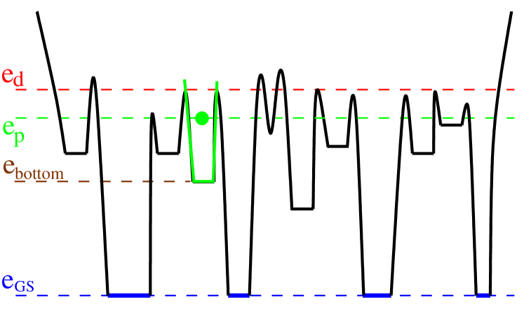
Figure 1: (color online) A cartoon of the energy landscape in mean field glassy systems. The different valleys correspond to different Gibbs states and are separated by extensive barriers. The cavity or replica method can compute how many states of a given entropy are present at a given energy/temperature). The following states method instead pins up one state (in green) that is one of the equilibrium ones at energy $e_{p}$ (or temperature $T_{p}$) and computes its properties (entropy, energy) for another temperatures $T$. At $T=0$, it leads the properties of the bottom of the state as e.g. the limiting energy $e_{\rm bottom}$.

1 Following Gibbs states

How to follow adiabatically a given Gibbs state? Consider first the two “up” and “down” equilibrium states in an Ising ferromagnet at low temperature. We can force the system to be in the Gibbs state of choice by fixing the all negative or all positive boundary conditions. Even far away from the boundaries, the system will stay in the selected state for all $T<T_{c}$ (above the Curie point $T_{c}$ any boundary condition will result in a trivial paramagnetic state). By solving the thermodynamics conditioned to the boundaries, we can thus obtain the adiabatic evolution of each of the two states.

What boundary conditions should be applied in glassy systems where the structure of Gibbs states is very complicated? The answer is provided by the following gedanken experiment [14]: Consider an equilibrium configuration of the system at temperature $T_{p}$. Now freeze the whole system except a large hole in it. This hole is now a sub-system with a boundary condition typical for temperature $T_{p}$. If the system is in a well-defined state, then no matter the size of the hole, it will always remain correlated to the boundaries and stay in the same state. One may now change the temperature and study the adiabatic evolution of this state. This can be achieved through Monte-Carlo simulations in any model. We shall here instead concentrate on mean-field systems, where this construction allows for an analytic treatment in the spirit of the cavity method [15, 16].

2 Mean field glassy models

We focus on two of the most studied mean field glassy systems: the Ising $p$-spin [17] and the Potts glass [18] models. These are also of fundamental importance in computer science where they are known as the XOR-SAT [19] and coloring [20] problems. Consider a graph defined by its vertices $i=\{1,\dots,N\}$ and edges $(i,j)\in{\cal E}$, the coloring Hamiltonian reads

$${\cal H}(\{s\})=\sum_{(i,j)\in{\cal E}}\delta(s_{i},s_{j})\,,$$ (1)

where $s=1,\ldots,q$ are the values of the Potts spins. The Ising $p$-spin is defined on a hyper-graph with $N$ vertices and $M$ $p$-body interactions (or constraints, if only zero energy configurations are of interest) with the Hamiltonian

$${\cal H}(\{s\})=-\sum_{a=1}^{M}J_{a}\prod_{i\in\partial a}s_{i}\,,$$ (2)

where $s=\pm 1$, $\partial a$ is the set spins involved in interaction $a$, and $J_{a}=\pm 1$ are chosen uniformly at random. For XOR-SAT, one defines instead the number of unsatisfied constraints $E_{\rm xor}=(M+E_{\rm p-spin})/2$, hence for XOR-SAT also the temperature is divided by a factor $2$ with respect to the $p$-spin model. With these definitions, the XOR-SAT and coloring problems are said to be satisfied if the ground state energy is zero. In both cases, we will consider the lattice to be a random (hyper-)graph with fixed degree $c$, i.e. every variable being involved in $c$ interactions, in the thermodynamic limit, $N\to\infty$. We also consider the large connectivity $c\to N^{p-1}/(p-1)!$ limit of (2) with $J_{a}=\pm\sqrt{p!}/(\sqrt{2N^{p-1}})$: the “fully-connected” $p$-spin model [17].

3 Cavity equations for following states

We now derive the state-following equations for $T_{p}\geq T_{K}$ in the XOR-SAT problem. This derivation can be generalized for $T_{p}<T_{K}$, and for any model where the cavity approach [6] can be applied, and this shall be detailed elsewhere [21].

As a large random (hyper-)graph is locally tree-like, let us thus first consider the problem on a large (hyper-)tree (see Fig. 2). Once the proper boundary conditions are chosen, computations on the tree give correct results for large random graphs: this is the basis of the cavity approach.

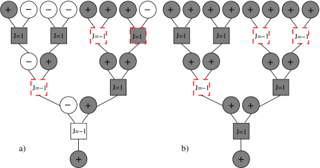
Figure 2: (color online) a) Recursive construction of an equilibrium configuration at temperature $T_{p}$ in XOR-SAT. Given the tree, and a random choice of interactions (full square $J=1$, empty square $J=-1$), one starts from the root, and chooses iteratively the configuration of ancestors (full circles $s=1$, empty circle $s=-1$) randomly such that it satisfies the constraints with probability $1-\epsilon(T_{p})$ (here $\epsilon=3/7$). Violated constraints have dashed/red borders. b) The problem can also be Gauge transformed into a fully polarized configuration with all $s=1$ but where the $J$’s are chosen from $P_{p}(J)=\epsilon(T_{p})\delta(J+1)+[1-\epsilon(T_{p})]\delta(J-1)$.

We derive the method of following states for the p-spin Hamiltonian (2). We concentrate on an equilibrium state at $T_{p}$, with $T_{p}\!\geq\!T_{K}$, where the equilibrium solution is given by the replica symmetric (RS) cavity method, or equivalently by the fixed point of the Bethe-Peierls (or Belief Propagation, BP) recursion [19]:

$$\beta h^{i\to a} =\sum_{b\in\partial i\setminus a}{\rm atanh}{\big{[}\tanh{(\beta J_{b})}\prod_{j\in\partial b\setminus i}\tanh{(\beta h^{j\to b})}\big{]}}{\equiv}$$

$${\equiv\beta{\cal F}(\{h^{j\to b}\},\beta)}\,,$$ (3)

where $h^{i\to a}$ is an effective cavity field seen by the spin $i$ due to all its neighboring spins $j$ except those connected to the interaction $a$; by $\partial i\setminus a$ we denote all interaction in which spin $i$ is involved except $a$. For $T_{p}\!\geq\!T_{K}$ the effective field $h^{i\to a}\!=\!0$ for all edges $ia$, and the fraction of violated constraints is hence $\epsilon(T_{p})=(1+e^{2/T_{p}})^{-1}$ [19].

One can generate an equilibrium configuration on a tree once the effective fields are known[15] using the iterative procedure described in Fig. 2. The values assigned to the variables on the leaves are then fixed and the measure they induce in the bulk of the tree defines an equilibrium Gibbs state at temperature $T_{p}$. As long as $T_{p}\geq T_{K}$, the computation in the bulk of the tree describes correctly the properties of the problem on the random graph.

All the properties of the Gibbs state are thus obtained by solving the BP equations initialized in this boundary configuration. When $T=T_{p}\geq T_{K}$, the results of the usual 1RSB calculation are recovered, as first discussed in the context of reconstruction on trees [15]. For $T=T_{p}>T_{d}$ BP will converge back to $h^{i\to a}\!=\!0$ for all edges $ia$, but when $T_{d}\geq T=T_{p}\geq T_{K}$, the configuration we picked lies in one of the exponentially many equilibrium Gibbs states and the BP fixed point thus describes one of them.

Now is the new crucial turn: Since the boundary conditions define the equilibrium Gibbs state at $T_{p}$, we can use the BP equations (3) initialized in the boundary condition but with a different temperature $\beta=1/T\neq 1/T_{p}$. The resulting fixed point now describes the properties of the very same state but at a different temperature $T\neq T_{p}$.

This line of reasoning translates readily in a set of coupled recursive cavity equations, which are a two-temperatures extension of the reconstruction formalism [15, 16]. Two distributions of fields $P_{s}(h)$, with $s=\pm 1$ depending on whether the site was set $\pm 1$ in the broadcasting, are given by

$$P_{s}(h)=\sum_{J_{a}}P(J_{a})\sum_{\{s_{i}\}}\frac{e^{\beta_{p}J_{a}s\prod_{i}s_{i}}}{2^{p-1}\cosh{\beta_{p}}}\times$$

$$\int\prod_{i=1}^{p-1}\prod_{j_{i}=1}^{c-1}{\rm d}P_{s_{i}}(h^{j_{i}})\,\delta[h-{\cal F}(\{h^{j_{i}}\},\beta)]\,,$$ (4)

where the delta function ensures that cavity field $h$ is related to the fields $h^{j_{i}}$ via eq. (3). The term in front of the integral describes the properties of the equilibrium configuration at inverse temperature $\beta_{p}$. Eq. (4) describes adiabatic evolution of a Gibbs state that is one of the equilibrium ones at $\beta_{p}<\beta_{K}$ in the $p$-spin model with distribution of interaction strength $P(J_{a})=\rho\delta(J-1)+(1-\rho)\delta(J+1)$, it can be solved numerically using the population dynamics technique [6]. The (Bethe) free energy of the same state at the new temperature $T$ reads

$$\beta f_{\beta_{p}}(\beta)\!\!\!\! \!\!\!\!=\frac{c-1}{2}\sum_{s_{i}}\int\prod_{i=1}^{c}{\rm d}P_{s_{i}}(h^{i})\log{Z^{i}}-\frac{c}{p}\sum_{J_{a}}P(J_{a})$$ (5)

$$\!\!\!\!\sum_{\{s_{i}\}}\frac{e^{\beta_{p}J_{a}\prod_{i}s_{i}}}{2^{p}\cosh{\beta_{p}}}\int\prod_{i=1}^{p}\prod_{j_{i}=1}^{c}{\rm d}P_{s_{i}}(h^{j_{i}})\log{Z^{a+\partial a}}\,,$$

where the $Z$’s are

$$Z^{a+\partial a}\!\!\!\! = \!\!\!\!\frac{\cosh(\beta J_{a})\prod_{i\in\partial a}2\cosh(\beta h^{i\to a})}{\prod_{i\in\partial a}\prod_{b\in\partial i\setminus a}2\cosh(\beta u^{b\to i})}[1+\tanh{(\beta u^{a})}]\,,$$

$$Z^{i}\!\!\!\! = \!\!\!\!2\cosh{(\beta\sum_{b\in\partial i}u^{b\to i})}\prod_{{b\in\partial i}}\frac{1}{2\cosh{\beta u^{b\to i}}}\,,$$ (6)

where $\tanh{(\beta u^{b\to i})}=\tanh{(\beta J_{b})}\prod_{j\in\partial b\setminus i}\tanh{(\beta h^{j\to b})}$.

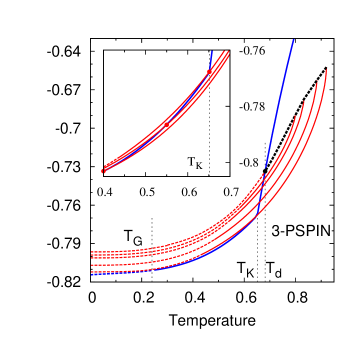
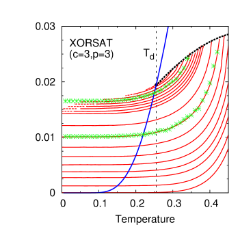
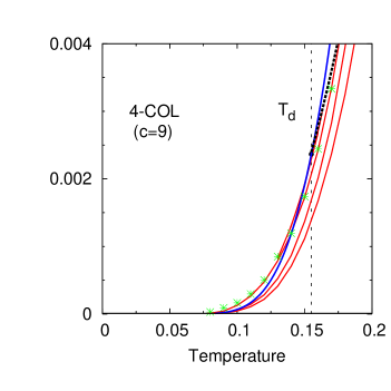
Figure 3: (color online) Behavior of Gibbs states in mean field glassy systems: the energy $e$ is plotted as a function of temperature $T$. The equilibrium energy (blue) is shown, together with the energy of several states (red) bellow the dynamical transition where we follow them out-of-equilibrium. States can be followed a) upon heating until a spinodal point (black-dotted curve) and b) upon cooling until they reach their bottom at zero temperature. However, the states closer to $T_{d}$ undergo a FRSB transition upon cooling and divide into many marginally stable sub-states at a temperature $T_{m}<T_{p}$ (red-dotted curve). Left: the fully-connected 3-spin model with its dynamical $T_{d}$, Kauzmann $T_{K}$ and Gardner $T_{G}$ (equilibrium states becoming FRSB [11]) transitions. We have used the 1RSB formalism to follow all the states down to zero temperature. The uppermost point at $T=0$ thus gives a 1RSB lower bound on the limiting energy of an adiabatically slow simulated annealing. Inset: the behavior of states for $T_{p}<T_{K}$, explicitly demonstrating the presence of temperature chaos. Middle: the XOR-SAT problem for $p=3,c=3$ where $T_{K}=0$. Again, the higher energy states become unstable, here we used only the RS formalism and thus were not able to continue all of them to zero temperature. In this model all $T_{p}>0$ states finish at a finite bottom energy at $T=0$. Right: The $4$-coloring of graphs with degree $c=9$. The situation is similar to the XORSAT case except that here all the states have their energy decaying very fast to zero when $T\to 0$. Asterixes (green) represent the results of adiabatic simulations starting from an equilibrated configuration on a $N=10^{5}$ graph using Monte-Carlo (in XORSAT) and BP (in coloring) evolution.

4 Gauge transformation

In the $p$-spin model, the above equations can be further simplified by exploiting a Gauge invariance. For any spin $i$, the Gauge transformation $s_{i}\to-s_{i}$ and $J_{ij}\to-J_{ij}$ for all $j\in\partial i$ keeps the Hamiltonian eq. (2) invariant. As shown in Fig. 2, this allows to transform the equilibrium spin configuration into a uniform one (all $s=1$), the disorder distribution then changes to $P_{p}(J)$ (see Fig. 2). Since all $s=1$, there is no need to distinguish between the $+1$ and the $-1$ sites, and eq. (4) reduces to the usual replica symmetric cavity equation for a problem with mixed ferromagnetic/anti-ferromagnetic interactions at temperature $T$ initialized in the uniformly positive state, where the distribution of interactions is given by the Nishimori-like [22] condition $P(J)=\epsilon(T_{p})\delta(J+1)+[1-\epsilon(T_{p})]\delta(J-1)$.

The Gauge invariance have thus transformed the task of following an equilibrium state in a glassy model into simply solving a known ferromagnetically biased model with the standard cavity approach. One can show in particular that following states in the fully connected $p$-spin model for $T_{p}\geq T_{K}$ is equivalent to solving the $p$-spin model with an additional effective ferromagnetic coupling $\langle J_{a}\rangle N^{p-1}/p!=J_{0}^{\rm eff}=\beta_{p}^{2}/2$, and one can thus readily take the solution of the p-spin in the literature, e.g. [17], to obtain properties of equilibrium states.

5 Energy landscape

We now present the results of the above formalism for the fully connected $3$-spin problem, the XOR-SAT with $c=3,p=3$ and the $4$-coloring of graphs with degree $c=9$. Fig. 3 shows the energy density $e(T)$ for several Gibbs states, that are the equilibrium ones at $T=T_{p}$, as they become out-of-equilibrium at $T\neq T_{p}$. Although such plots were often presented as sketches in previous works, analytical results were so far available only for few very simple models [7, 12].

We confirmed that glassy equilibrium Gibbs states exist only for $T_{p}\leq T_{d}$ while for $T_{p}>T_{d}$ we saw only the liquid solution. As these states are heated, they can be followed until a well-defined spinodal temperature $T_{s}(T_{p})$ that grows as $T_{p}$ decreases (this is reminiscent of the Kovacs effect in glassy materials [23]). Interestingly we find that $T_{s}(T_{p}=T_{d})=T_{d}$, i.e. an equilibrium state at $T_{d}$ disappears (melts) for any increase of temperature, this is at variance with the (unphysical) behavior in spherical models where such a state exists until much larger $T$ [12].

We also consider the state evolution upon cooling. As anticipated based on the statistical features of the energy landscape [24] and the study of spherical models [7, 12], we find that for $T_{p}$ near enough the dynamical temperature $T_{d}$, the states undergo a FRSB transition: at some $T_{m}<T_{p}$ the states decompose into many marginally stable sub-states [11]. In such a case the exact solution for adiabatic evolution requires the FRSB approach [5] and our RS approach yields only a lower bound on the true energy. Moreover, for temperatures slightly below the FRSB instability, the RS solution undergoes an unphysical spinodal transition and we are thus unable to obtain even the RS lower bound. For the fully connected $p$-spin model we have therefore used the 1RSB formalism (using the mapping onto the ferromagnetic-biased model) which allowed us to follow states until $T=0$ (see Fig. 3, right panel). The FRSB solution is numerically much more involved, making the exact analysis obviously more difficult.

Note that following the evolution of a state that is the equilibrium one at $T_{p}=T_{d}$ is particularly interesting. An adiabatically slow annealing is able to equilibrate down to $T_{d}$ and the evolution of the state at $T_{d}$ is thus giving the asymptotic behavior of the simulated annealing algorithm.

To assess the validity of our approach, we have performed numerical simulations. For models such as XOR-SAT and coloring for $T\geq T_{K}$, where the annealed average is equal to the quenched average, it is possible to use the quiet planting trick [16] to generate an equilibrated configuration together with a typical random graph: Starting with a random configuration one simply creates the (hyper-)graph randomly such that the configuration has $\epsilon(T_{p})N$ violated constraints. As seen in Fig. 3, when initialized in $T_{p}\in[T_{d},T_{K}]$, the evolution upon heating and cooling, simulated both by BP and slow Monte-Carlo simulations, follows precisely our predictions.

Finally, we have also consider the adiabatic following of states for $T_{p}<T_{K}$. Their behavior is depicted in the inset of the left panel in Fig. 3. At variance with the situation in spherical models [12], these states become out-of-equilibrium as soon as the temperature is changed. The equilibrium configurations for $T<T_{K}$ thus do not belong to a single state, but instead to a succession of many different states whose free energies cross as $T$ changes: This demonstrates explicitly the presence of temperature chaos in the static glass phase $T<T_{K}$ [13].

6 Comparison with previous approaches

How do our results compare with previous heuristic approaches to adiabatic annealings? Two arguments have been mainly proposed. The first one is the marginality criterion [8] according to which the energy reached by a slow annealing at zero temperature can be computed by sampling a typical energy minima at a given energy $e$, and then choosing $e$ such that this minima is marginally stable with respect to the replica symmetry breaking. This uniform minima-sampling argument is, however, unjustified, since the dynamics always goes in out-of-equilibrium states bellow $T_{d}$. Indeed, as already shown by [24], the marginality criterion is not correct and its result not consistent.

A refined approach called iso-complexity was thus introduced in [24]. It is proposed to count the number of equilibrium states at a given $T_{p}$, and then to consider the energies at $T<T_{p}$ for which the number of states is equal to the one at $T_{p}$. Iso-complexity leads indeed to a lower bound on adiabatic annealings, because in order to end up at lower energies one would have to be exponentially lucky. With our formalism (where we explicitly follow states) we checked that adiabatic annealings always ends up at higher energies than the iso-complexity ones. This is illustrated in Fig. 4, where we show the energy of the bottoms of states that are the equilibrium ones at temperature $T_{p}$ and compare it to the iso-complexity result (that gives strictly lower values). Unfortunately the RSB instability within states mentioned previously prevents us from estimating the asymptotic energy when $T_{p}$ is close to $T_{d}$.

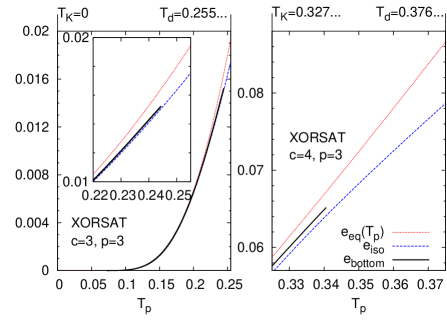
Figure 4: (color online) Comparison between the exact adiabatic evolution of states and the iso-complexity lower bound. The black line is the energy of the bottoms of states that were the equilibrium ones at temperature $T_{p}\in[T_{K},T_{d}]$ in XOR-SAT for $c=3$, $p=3$ (left, the inset is a zoom) and for $c=4$, $p=3$ (right). The red (upper-most) line is the equilibrium energy at $T_{p}$. The blue line is the iso-complexity lower bound [24].

7 Canyons versus valleys

An important class of mean field glassy models are the constraint satisfaction problems where one searches for a configuration satisfying all the constraints. As opposed to early predictions [3], it has been observed that glassiness does not prevent simple algorithms from finding a ground state [20, 25]. The following state method allows to understand this fact and to shed light on the energy landscape of these problems. Indeed, we see in Fig. 3 that although in the XOR-SAT problem all the typical finite $T_{p}$ equilibrium states have their bottoms at positive energies, the situation is different in $4$-coloring with $c=9$ where all depicted states descent to zero energy when the temperature is lowered.

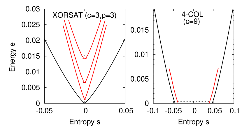
Figure 5: (color online) Data from Fig. 3 plotted in order to visualize the energy landscape. The energy $e$ is plotted against the entropy $s=\beta(e-f)$ for different equilibrium states. We plotted $s(e)/2$ and $-s(e)/2$ such that the width corresponds to the logarithm of the number of configurations at energy $e$ for the Gibbs state. Left: XOR-SAT with $c=3$, $p=3$. Right: 4-coloring of random graphs with $c=9$. The black curve corresponds to the equilibrium total entropy. The red curves are different equilibrium states, corresponding to $T_{p}=0.15,0.2,0.24$ (left), and $T_{p}=0.12$ on (right), the energies corresponding to $T_{p}$ are depicted by horizontal black dashed lines. The left side states, with their finite energy bottoms, remind us of the valley in Fig. 1, while the right side reminds of deep canyons that all reach the ground state energy.

Looking back to Fig. 1, we see that the landscape has many valleys with bottoms at finite energies, but also canyon-shaped states that reach the ground state energy. We now define two types of glassy landscape: (1) In the canyons-dominated landscape, a typical (equilibrium) state at $T_{p}=T_{d}$ has its bottom at zero energy while (2) in the valleys-dominated landscape a typical equilibrium state at $T_{d}$ has its bottom at strictly positive energy.

In order to quantitatively observe canyons and valleys, we have computed the ”shape” of the states (see Fig. 5). For XOR-SAT at $c=3$, $p=3$ we observe the standard picture of valleys with bottoms at positive energy. In 4-coloring of graph with degree $c=9$, however, the states indeed have a canyon-like shape and go down to zero energy. While an adiabatic annealing would be stuck at finite energy in the first case, it would instead reach a solution (although not an equilibrium one) in the second one. This is not to say that $4$-coloring of graphs of degree $c=9$ is really easy (since we are speaking of an infinitely slow annealing procedure) but rather to explain based on analytical calculations why it is sometimes possible to find solutions even in the clustered glassy phase using simple local search algorithms, as observed in [20, 25].

In problems such as graph coloring or satisfiability of Boolean formulas, there will thus be a sharp transition (in general different from the clustering and the satisfiability transitions) as the constraint density is increased, where the energy landscape changes from canyon-dominated to valley-dominated one: this transition marks the onset of difficulty of the problem for an ideally slow annealing, and most likely also for other stochastic local search algorithms. This point can be in principle computed by the following state formalism, however, the replica-symmetry-breaking instability discussed above complicates the numerical resolution of the corresponding equations and we will thus discuss it elsewhere [21]. We also show explicitely in [21] that this transition is upper bounded by the so-called rigidity transition point where frozen variables appear in the equilibrium ground state configurations [20, 26]. This further supports the conjecture of [20] that solutions with frozen variables are really hard to find.

Another observation can be made from Fig. 3: Even if one equilibrates the system at $T=T_{d}$, the state soon becomes unstable towards FRSB upon cooling. Therefore any cooling procedure will end up at best in far from equilibrium FRSB states. This shows how futile are the attempts to study equilibrium predictions, such as the appearance of clustering or BP fixed points, starting from solutions obtained by heuristics solvers that performing a kind of annealing in the landscape. Instead typical configuration must be obtained. This can be achieve by Monte-Carlo, or using exhaustive search [27] for small instances, or by planting[16] for larger ones (as we did in Fig.3.)

8 Conclusions

We have described how to follow adiabatically Gibbs states in glassy mean field models, and answered some long-standing questions on their energy landscape: We have discussed the residual energy after an adiabatically slow annealing, the behavior of out-of-equilibrium states, and demonstrated the presence of temperature chaos. We have also found new features of the energy landscape, and identified a transition from a canyons-dominated landscape to a valleys-dominated one.

The following state method presented here has a wide range of applications and we believe that many mean fields model will profit from being revisited in these directions.

References

- [1] M. Mézard and G. Parisi, Phys. Rev. Lett. 82, 747 (1999). G. Parisi and F. Zamponi, Rev. Mod. Phys. 82, 789 (2010). E. Shakhnovich and A. M Gutin, J. Phys. A: Math. Gen, 22 1647-1659 (1989).
- [2] M. Mézard and A. Montanari, Physics, Information, Computation, Oxford Press 2009.
- [3] M. Mézard, G. Parisi and R. Zecchina, Science 297, 812 (2002).
- [4] F. Krzakala et al., Proc Natl Acad Sci USA 104, 10318 (2007).
- [5] M. Mézard, G. Parisi, and M. A. Virasoro, Spin Glass Theory and Beyond, World Scientific, Singapore, (1987).
- [6] M. Mézard and G. Parisi, Eur. Phys. J. B 20 217 (2001).
- [7] L. Cugliandolo and J. Kurchan, Phys. Rev. Lett. 71, 173 (1993).
- [8] J.-P. Bouchaud et al, in Spin Glasses and Random Fields, edited by A. P. Young (World Scientific, Singapore, 1998).
- [9] A. Montanari and G. Semerjian, J. Stat. Phys. 124, 103 (2006).
- [10] W. Kauzmann, Chem. Phys. 43 219 (1948). R. Monasson, Phys. Rev. Lett. 75, 2847 (1995).
- [11] E. Gardner, Nuclear Physics B 257, 747 (1985).
- [12] A. Barrat, S. Franz and G. Parisi, J. Phys. A: Math. Gen. 30 5593 (1997). B. Capone et al. Phys. Rev. B 74, 144301 (2006).
- [13] F. Krzakala and O. C. Martin Eur. Phys J. B 28, 199 (2002). T. Rizzo and H. Yoshino, Phys. Rev. B 73, 064416 (2006). T. Mora and L. Zdeborová, J. Stat. Phys. 131 6, 1121 (2008).
- [14] J.-P. Bouchaud and G. Biroli, J. Chem. Phys. 121, 7347 (2004).
- [15] M. Mézard and A. Montanari, J. Stat. Phys. 124, 1317 (2007).
- [16] F. Krzakala and L. Zdeborová, Phys. Rev. Lett. 102, 238701 (2009) and arxiv:0902.4185.
- [17] B. Derrida, Phys. Rev. Lett. 45, 79 (1980). D.J. Gross and M. Mézard, Nucl. Phys. B, 240 (1984) 431.
- [18] F. Krzakala and L. Zdeborová, EPL 81 57005 (2008).
- [19] F. Ricci-Tersenghi, M. Weigt and R. Zecchina, Phys. Rev. E 63, 026702 (2001).
- [20] L. Zdeborová and F. Krzakala, Phys. Rev. E 76 031131 (2007).
- [21] F. Krzakala and L. Zdeborová, arXiv:1003.2748v1.
- [22] H. Nishimori, Prog. Theor. Phys. 66, 1169 (1981).
- [23] A. J. Kovacs, Adv. Polym. Sci. 3, 394 (1963).
- [24] A. Montanari and F. Ricci-Tersenghi, Phys. Rev. B 70, 134406 (2004) and Eur. Phys. J. B 33, 339 (2003).
- [25] J. Ardelius and E. Aurell, Phys. Rev. E 74, 037702, 2006. F. Krzakala and J. Kurchan, Phys. Rev. E 76, 021122 (2007). L. Dall’Asta, A. Ramezanpour and R. Zecchina, Phys. Rev. E 77, 031118 (2008).
- [26] G. Semerjian, J. Stat. Phys. 130, 251 (2008)
- [27] J. Ardelius and L. Zdeborová, Phys. Rev. E 78, 040101 (2008).