Polarization properties in the transition from below to above lasing threshold in broad-area vertical-cavity surface-emitting lasers

Abstract

For highly divergent emission of broad-area vertical-cavity surface-emitting lasers (VCSELs) a rotation of the polarization direction by up to 90 degrees occurs when the pump rate approaches the lasing threshold. Well below threshold the polarization is parallel to the direction of the transverse wave vector and is determined by the transmissive properties of the Bragg reflectors that form the cavity mirrors. In contrast, near-threshold and above-threshold emission is more affected by the reflective properties of the reflectors and is predominantly perpendicular to the direction of transverse wave vectors. Two qualitatively different types of polarization transition are demonstrated: an abrupt transition, where the light polarization vanishes at the point of the transition, and a smooth one, where it is significantly nonzero during the transition.

I Introduction

In the last decades vertical cavity surface emitting lasers (VCSELs) have played an increasing role in scientific research and applications Wilmsen et al. (1999). One of the features of VCSEL design is the possibility to obtain large two-dimensional apertures which are quite homogeneous and have a small polarization anisotropy.

The polarization behavior in such lasers resulting from the competition of stimulated and spontaneous emission has been a subject of many investigations Mulet et al. (2001); Hermier et al. (2002); Willemsen et al. (2001); Shelly et al. (2000); Golubev et al. (2004). It is known that the polarization properties of small and medium aperture VCSELs above Miguel et al. (1995); Travagnin et al. (1996); Travagnin (1997); Sondermann et al. (2003); Balle et al. (1999); Panajotov et al. (2000) and below Willemsen et al. (2001); Shelly et al. (2000) threshold are determined mainly by the intracavity anisotropies. Well below threshold the polarization degree is reduced dramatically, in VCSELs Willemsen et al. (2001) as well as in edge-emitting semiconductor lasers Ptashchenko (1996) (which possess much higher intracavity anisotropies). However, below threshold the polarization coincides with the at-threshold one.

With increasing size of the aperture, off-axis emission becomes important. Because the cavity resonance is different for different transverse modes, the ones with the best alignment between the cavity resonance and the gain maximum of the active medium have the largest gain Moloney and Newel (1990); Jakobsen et al. (1992). Recently it was shown Hegarty et al. (1999a); Loiko and Babushkin (2001a); Babushkin et al. (2008) that for strongly off-axis emission the intra-cavity anisotropies play only an auxiliary role in polarization selection above threshold. In contrast, the polarization-selective properties of reflection and transmission of the distributed Bragg reflectors (DBRs) forming the cavity mirrors are much more important. Above threshold, the DBR TE modes (which are in paraxial approximation perpendicular to the transverse component of the wave vector, i.e. s-waves) have higher reflectivity, and the cavity quality factor for the TE modes is larger than for the TM modes. This determines the polarization of the above threshold emission, which has an overall tendency to be perpendicular to the transverse wave vector (“90-degree rule”) Loiko and Babushkin (2001a). Later investigations established that the above-threshold polarization is also strongly affected by the transverse cavity boundaries, i.e. the waveguide formed by the oxide confinement Babushkin et al. (2008). This leads to strong deviations of the above-threshold polarization state from the “90-degree rule” for transverse wave vectors with directions not parallel to either of the device boundaries Babushkin et al. (2008). The data in Babushkin et al. (2008) (for lasers with a square aperture) and in Schulz-Ruhtenberg et al. (2009) (for lasers with a circular aperture) indicate also that the polarization direction for off-axis light is different below and above threshold but there is no detailed investigation.

In this work we characterize the polarization properties of off-axis below-threshold emission and show that the polarization direction is governed mainly by the transmissive properties of the top DBR. The transmissivity is larger for the TM Bragg modes (parallel to the transverse wave vector, p-waves) than for the s-waves, resulting in a “0-degree rule” for polarization selection, i.e. the polarization is parallel to the transverse wave vector.

We consider, both theoretically and experimentally, the transition from the below-threshold to the above-threshold polarization state for highly divergent VCSEL emission. The nature of the transition depends critically on the orientation of the polarization of the final (lasing) state. When the final polarization obeys the “90-degree rule” and is perpendicular to the polarization state well below threshold, the transition is very abrupt and the light is unpolarized at the point of transition. On the other hand, when the polarization of final state is not orthogonal to the initial one, the transition is considerably smoother, and the emission retains a relatively large degree of polarization during the transition. Our theory predicts also that far below threshold the main principal axes of the intra-cavity and extra-cavity field are perpendicular to each other due to the strong anisotropic filtering of the light coupled out via the DBRs.

In the next section we describe the experimental setup; in Sect. III the experimental results are reported. In Sect. IV a theoretical model for the description of the transition is developed, analyzed and the results compared to the experimental observations. Concluding remarks are in Sect. V.

II Experimental setup and methods

The VCSELs under study are oxide-confined top-emitters with a square aperture of $40\times 40\text{\,}{\mathrm{\SIUnitSymbolMicro m}}^{2}$ that are packaged in TO-type housings without caps. The emission wavelength is around $780\text{\,}\mathrm{nm}$. The lasers consist of two highly reflective DBRs (top mirror: 31 layers, bottom mirror: 47 layers) with three $8\text{\,}\mathrm{nm}$ thick Al_0.11Ga_0.89As quantum wells in between. Together with several Al_0.36Ga_0.64As spacer layers and the GaAs substrate the whole structure is about $10\text{\,}\mathrm{\SIUnitSymbolMicro m}$ long. In order to reduce the electrical resistance of the lasers the interfaces between different semiconductor layers are graded. A laterally oxidized layer above the active region provides current and optical confinement.

The devices are electrically pumped with a low-noise DC current source between 0 and $30\text{\,}\mathrm{mA}$. The typical lasing threshold at $0\text{\,}\mathrm{\SIUnitSymbolCelsius}$ heat sink temperature is $15\text{\,}\mathrm{mA}$. The VCSEL is mounted on a copper plate that is attached to a thermo-electric cooling element enabling temperature control between $40\text{\,}\mathrm{\SIUnitSymbolCelsius}$ and $-35\text{\,}\mathrm{\SIUnitSymbolCelsius}$. We remark that the actual device temperature is strongly influenced by the driving current due to Joule heating effects. Temperature values given here are for the heat sink only. The device temperature can be inferred indirectly from optical spectra and changes with current by a factor of about 0.9 K/mA. The device temperature changes the detuning between the cavity resonance and the maximum gain frequency, since these shift with distinctly different rates with temperature (typical values are $0.28\text{\,}\mathrm{nm}\text{\,}{\mathrm{K}}^{-1}$ for the gain peak and $0.075\text{\,}\mathrm{nm}\text{\,}{\mathrm{K}}^{-1}$ for the resonance, e.g. Hegarty et al. (1999b)). As considered in detail in Schulz-Ruhtenberg et al. (2005) this mechanism controls the length scales of the transverse patterns emitted by the VCSEL.

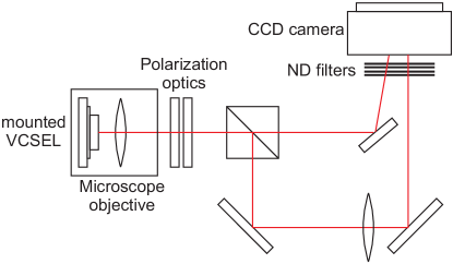
Figure 1: (Color online) Experimental setup. The VCSEL is set into an air-tight box to avoid condensation water. Polarization optics: half-wave plate and linear polarizer.

Figure 1 shows the setup used for the experiments. The laser beam is collimated by a microscope objective with a numerical aperture of 0.8. VCSEL, cooling elements, and the objective are put into an air-tight box to avoid condensation of water at low temperatures. The far-field of the laser emission is imaged onto a high-resolution 14-bit camera with a large charge-coupled device (CCD) chip. A half-wave plate and a linear polarizer are inserted into the beam path. The orientation of the polarizer defines the reference coordinate system by which the state of polarization is represented. Horizontal polarization is defined as 0^∘, angles are measured in counter-clockwise direction. The polarization is measured by taking far-field images for three settings of the polarization optics: horizontal ($I_{x}$), vertical ($I_{y}$), and diagonal orientation ($I_{45}$). For the circular component ($I_{circ}$) a quarter-wave plate (set to 45^∘ with respect to the horizontal) is necessary. From this data, the spatial-resolved Stokes parameters are calculated:

$$\begin{split}&S_{0}=I_{x}+I_{y},\;S_{1}=\frac{(I_{x}-I_{y})}{S_{0}},\;\\ &S_{2}=\left(\frac{2\cdot I_{45}}{S_{0}}\right)-1,\;S_{3}=\left(\frac{2\cdot I_{circ}}{S_{0}}\right)-1,\end{split}$$ (1)

where $S_{0}$ represents the total intensity, $S_{1}$ the (normalized) amount of light polarized in $x$ (positive $S_{1}$) respectively $y$ (negative $S_{1}$) direction, $S_{2}$ the (normalized) amount of light polarized along the diagonal direction (positive for 45^∘, negative for -45^∘) and $S_{3}$ the (normalized) amount of circularly polarized light (the sign denotes the direction of rotation). Using this set of Stokes parameters the degree of polarization (fractional polarization) $p$ and the polarization direction $\varphi$ can be calculated:

$$p=\sqrt{S_{1}^{2}+S_{2}^{2}+S_{3}^{2}},\,\varphi=\frac{1}{2}\cdot\arctan(\frac{S_{2}}{S_{1}}).$$ (2)

The fraction of circular polarization $S_{3}$ was found to be of the order of 0.02, thus we assume linear polarization in the following. In this article we focus on the characteristics of two VCSELs, which illustrate the general behavior found in the experiments very well.

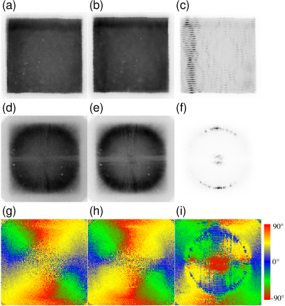
Figure 2: (Color online) Near- and far-field images for device #1 below and above threshold. Heat sink temperature $T$=$0\text{\,}\mathrm{\SIUnitSymbolCelsius}$ and driving current $12.0\text{\,}\mathrm{mA}$ (a,d,g), $13.5\text{\,}\mathrm{mA}$ (b,e,h), and $15.6\text{\,}\mathrm{mA}$ (c,f,i). The color-code of the polarization direction distribution (lowest row) is shown by the bar on the lower right. These images correspond to the transition shown in Fig. 5.

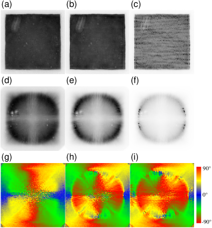
Figure 3: (Color online) Near- and far-field images for device #2 below and above threshold. Heat sink temperature $T$=$0\text{\,}\mathrm{\SIUnitSymbolCelsius}$ and driving current $13.5\text{\,}\mathrm{mA}$ (a,d,g), $15.5\text{\,}\mathrm{mA}$ (b,e,h), and $16.0\text{\,}\mathrm{mA}$ (c,f,i). The white spots in (a,b) result from debris on the neutral density filters. The color code is the same as in Fig. 2. These images correspond to the transition shown in Fig. 6.

III Distribution of spontaneous emission and the transition through threshold

We consider two nominally identical devices from the design and growth process, which show however rather different behavior. The near-field and far-field intensity distributions of the emission are shown in the figures 2 (device #1), resp. 3 (device #2). In both cases the heat sink temperature is $T$=$0\text{\,}\mathrm{\SIUnitSymbolCelsius}$, the threshold current for device #1 is $15.2\text{\,}\mathrm{mA}$, for device #2 $15.6\text{\,}\mathrm{mA}$. The first and second rows of each figure depict the intensity distributions in grey-scale coding (black denoting the maximum intensity) of the near-field and far-field, respectively, the third shows the spatial frequency distribution of the polarization direction in a cyclic color-code (red denotes $\pm$90^∘, green -45^∘, blue 0^∘, and yellow +45^∘, cf. to the color bar on the right of Fig. 2). The columns show the emission below threshold (panels a, d, g; $12.0\text{\,}\mathrm{mA}$ for device #1, $13.5\text{\,}\mathrm{mA}$ for device #2), slightly below threshold (panels b, e, h; $13.5\text{\,}\mathrm{mA}$ and $15.5\text{\,}\mathrm{mA}$), and just above threshold (panels c, f, i; $15.6\text{\,}\mathrm{mA}$ and $16.0\text{\,}\mathrm{mA}$). The optical axis is positioned in the center of each image.

Below and above threshold, the emission has its maximum at a well-defined wave number. This critical wave number is favored because it has the most favorable detuning properties as discussed above (see Schulz-Ruhtenberg et al. (2005) for details about the dependence of the transverse wave numbers of the emission on the detuning). Even far below threshold the ring indicating the critical wave number is easily discernible. With current approaching threshold it narrows until at threshold the lasing modes develop from this ring. This is easily explained by the increase of the Finesse of the cavity if threshold is approached.

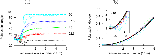
Figure 4: (Color online) Radial cuts (at 0^∘ (black solid line), 22.5^∘ (red long-dashed line), 45^∘ (green small-dashed line ), 67.5^∘ (blue dotted line), and 90^∘ (cyan dot-dashed line)) through the far-field distribution of the spontaneous emission for device #1. $T$=$0\text{\,}\mathrm{\SIUnitSymbolCelsius}$, $I$=$10\text{\,}\mathrm{mA}$. (a) Polarization in dependence on the transverse wave number $k_{\bot}$ showing the validity of the 0^∘-rule for $k_{\bot}>2\,\mu$m^-1. The thick lines indicate the polarization expected from the theory developed in Sect. IV. (b) Fractional polarization in dependence on $k_{\bot}$ for the same cuts as in (a). The part near $k_{\bot}\approx 0$ is shown in the inset.

Within this critical ring, far below threshold the maxima of spontaneous emission is found at the diagonals in Fourier space, but moves close to the axes above threshold (i.e. with either small $k_{x}$ for device #1 or $k_{y}$ for device #2). Just above threshold VCSEL #1 emits far-field patterns with two dominant Fourier components on the y-axis (Fig. 2(f)). The polarization of these components is in tendency orthogonal to their wave vector, which is shown in Fig. 2(i), where the area of lasing emission is polarized horizontally (blue in the color-code). Below threshold the polarization direction is very different, parallel to the wave vector (see Fig. 2(g)). These general observations are also true for device #2.

The validity of the ‘0^∘-rule’ is illustrated and tested further in Fig. 4. Here radial cuts through the polarization distribution at 0^∘, 22.5^∘, 45^∘, 67.5^∘, and 90^∘ with respect to the $x$-axis are shown for $T$=$0\text{\,}\mathrm{\SIUnitSymbolCelsius}$ and $I$=$10\text{\,}\mathrm{mA}$ (i.e. far below threshold). Each curve starts at about 10^∘ for $k_{\bot}\approx 0$ and switches asymptotically to the angle of the cut. For values of the transverse wave number above 1 $\mu$m^-1 the polarization is clearly parallel to the wavenumber. The deviations amount up to about 10^∘ at 1 $\mu$m^-1 and decrease for higher wave numbers. The polarization state at $k_{\bot}\approx 0$ is interpreted to be selected by the cavity anisotropies.

It is interesting to note that the curves of the polarization angle as well as the fractional polarization are continuous till the maximum value measured of 5 $\mu$m^-1 though between 3.5 $\mu$m^-1 and 5 $\mu$m^-1 (depending on the direction of the wave vector) the cutoff condition for the transverse modes of the waveguide formed by the refractive index step (i.e. the side boundaries formed by oxidation) sets in. It is clearly visible in the center rows of Figs. 2 and 3 that the intensity is cut-off indeed. This indicates that the influence of the side boundaries on the polarization characteristics of below-threshold emission is very small.

The fractional polarization, i.e. the amount of linearly polarized light, in dependence on the transverse wave number is shown in Fig. 4(b), again for the same cuts. It increases monotonically with wavenumber. The graphs are more or less congruent which indicates the isotropic character of the phenomenon, showing its relative independence from the principal axes of the intra-cavity anisotropy for large enough wavenumbers. The polarization degree is small, but nonzero for $k_{\bot}=0$ (see inset to Fig. 4(b)), which also indicates the influence of the cavity anisotropies, because the DBRs are isotropic for $k_{\bot}=0$.

In the following, we take a closer look at the changes involved in the transition from spontaneous to lasing emission. This transition is illustrated in Fig. 5 for device #1 and Fig. 6 for device #2. Each figure shows in (a) the local (in Fourier space) intensity, in (b) the fractional polarization, and in (c) the local polarization orientation in dependence on the driving current. In addition the pump rate

$$P=\frac{\left(I-I_{th}\right)}{I_{th}}$$ (3)

is displayed on the upper x-axis of the diagrams. The inset in (a) shows the Fourier component for which these plots were made (indicated by the arrow). The black lines in the (a) panels show in both cases the typical behavior of a laser crossing threshold: A region of low emission intensity representing spontaneous emission and small slope is followed by a steeply increasing part indicating lasing emission. Threshold is extrapolated by a linear fit to this latter part and indicated by the dashed red line. The blue curves in Fig. 5 and 6 are calculated from equations (9), (12) and will be discussed in the theoretical section.

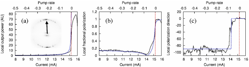
Figure 5: (Color online) Transition from spontaneous emission to lasing emission of the spot depicted in the inset in (a) for device #1. The black, solid curves are experimental data, the blue, dashed ones are calculated from Eqs. (9)-(12). (a) Local intensity in dependence on driving current. The threshold, indicated by the vertical red dashed line, is derived from a linear fit to the steep slope of the intensity. (b) Degree of polarization. (c) Local polarization direction. The change of polarization is evident about $1.5\text{\,}\mathrm{mA}$ below threshold.

The fractional polarization shown in (b) typically follows the development of the intensity until it saturates at a maximum of 0.8 to 1.0.

In part (c) of the figures the change of the polarization direction with current is shown. Far below threshold the polarization angle is in good agreement with the 0^∘-rule. With increasing current the scenario is different for the two lasers. For device #1, the polarization starts to change quite abruptly approximately $1.1\text{\,}\mathrm{mA}$ below threshold: In a current range of only $1\text{\,}\mathrm{mA}$ the angle changes to 0^∘, which corresponds to the “90-degree rule”. The polarization reaches the target state well below threshold (about 93% of $I_{th}$). Note that the fractional polarization has a pronounced local minimum at the transition.

Device #2 (Fig. 6(c)) shows a rather gradual change of the polarization that starts already more than $5\text{\,}\mathrm{mA}$ (at 67 % of $I_{th}$) below threshold. The behavior is monotonous, there is no dip in the fractional polarization. This behavior is typical, if the wavevector is not oriented along one of the two axis. Only in the latter case (Fig. 5) an abrupt transition is found. The continuous transition is more typical for the devices under study, though, because the wavevector configuration depicted in Fig. 6a is more typical Babushkin et al. (2008).

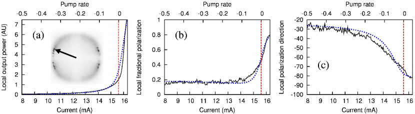
Figure 6: (Color online) Transition from spontaneous emission to lasing emission of the spot depicted in the inset in (a) for device #2. (a) Local intensity in dependence on driving current. (b) Degree of polarization. (c) Local polarization direction. All denotations are analogous to Fig. 5.

IV Theory and discussion

IV.1 The Ginsburg-Landau equation

In order to analyze the behavior described above we use a model for a broad-area VCSEL which accounts for its cavity structure including Bragg reflectors Loiko and Babushkin (2001a, b). For simplicity, we consider a spatially homogeneous device with an infinite aperture. For this case the eigenmodes are plane transverse waves ${\mathrm{\mathbf{E}}}_{{\mathrm{\mathbf{k}}}_{t}}(x,y,t)={\mathrm{\mathbf{E}(t)}}\exp\{i(k_{x}x+k_{y}y)\}$ where ${\mathrm{\mathbf{E}}}(x,y,t)\equiv\{E_{x},E_{y}\}$ is the slowly varying complex envelope of the field inside the cavity, ${\mathrm{\mathbf{k}}}_{\bot}=\{k_{x},k_{y}\}$ is the transverse component of the wave vector.

Many features of polarization selection at and slightly above threshold can be obtained by a linear stability analysis Babushkin et al. (2004, 2008). However, for the transition from below to above threshold it is of critical importance to take into account both spontaneous emission and the nonlinear saturation. Therefore we will use here a nonlinear Ginsburg-Landau equation (GLE) with an additional term describing spontaneous emission (see Appendix A for the derivation). For the spatially homogeneous device with infinite aperture the equation can be written for every transverse wave with complex amplitude ${\mathrm{\mathbf{E}}}(t)$:

$$\begin{split}\dot{{\mathrm{\mathbf{E}}}}=-\kappa_{\mathrm{in}}{\mathrm{\mathbf{E}}}-\kappa_{\mathrm{out}}\Upsilon({\mathrm{\mathbf{k}}}_{\bot}){\mathrm{\mathbf{E}}}+i\Omega({\mathrm{\mathbf{k}}}_{\bot}){\mathrm{\mathbf{E}}}+\Gamma{\mathrm{\mathbf{E}}}-\\ -\kappa_{\mathrm{out}}{\cal G}({\mathrm{\mathbf{k}}}_{\bot})I{\mathrm{\mathbf{E}}}+{\mathrm{\mathbf{W}}}.\end{split}$$ (4)

The field decay rate $\kappa=\kappa_{\mathrm{in}}+\kappa_{\mathrm{out}}$ results from the laser emission through the DBRs $\kappa_{\mathrm{out}}$ (outcoupling losses) and intracavity losses $\kappa_{\mathrm{in}}$ by scattering and absorption. The latter is isotropic (polarization independent), whereas the former is anisotropic. The anisotropy is described by the 2$\times$2-matrix $\Upsilon({\mathrm{\mathbf{k}}}_{\bot})$, which represents polarization- and ${\mathrm{\mathbf{k}}}_{\bot}$-dependent losses at the DBRs. In addition, the matrix $\Upsilon({\mathrm{\mathbf{k}}}_{\bot})$ includes also the gain in the device (and hence has a component depending linearly on the driving current). $\Omega({\mathrm{\mathbf{k}}}_{\bot})$ represents diffraction in the cavity and in the DBRs, $\cal{G}({\mathrm{\mathbf{k}}}_{\bot})$ is a matrix describing the impact of the nonlinear saturation and $I={\mathrm{\mathbf{E}}}^{\dagger}{\mathrm{\mathbf{E}}}$ is the light intensity ($\dagger$ means the conjugate transpose). A more detailed description of $\Upsilon({\mathrm{\mathbf{k}}}_{\bot})$, $\Omega({\mathrm{\mathbf{k}}}_{\bot})$ and $\cal{G}({\mathrm{\mathbf{k}}}_{\bot})$ is given in Appendix A. $\Gamma$ is the intracavity anisotropy matrix, which in the basis of the main anisotropy axes is written as $\Gamma=\mathrm{diag}\,(\gamma_{a}+i\gamma_{p},-\gamma_{a}-i\gamma_{p})$, where $\gamma_{a}$ is the amplitude anisotropy (dichroism), $\gamma_{p}$ is the phase anisotropy (birefringence) and $\mathrm{diag}\,(\cdot,\cdot)$ denotes a diagonal matrix with the corresponding entities on the diagonals.

As indicated above, the other source of anisotropy is the reflection at the DBRs. The action of the DBRs can be described in terms of s- and p-waves Born and Wolf (1980); Babic et al. (1993), which are plane transverse waves with polarization correspondingly perpendicular and parallel to the direction of the transverse wave vector ${\mathrm{\mathbf{k}}}_{t}$. In this basis, the matrix of reflection from the $i$th Bragg reflector is diagonal $R_{i}({\mathrm{\mathbf{k}}}_{t})=\mathrm{diag}\,\left\{R_{si}({\mathrm{\mathbf{k}}}_{t}),R_{pi}({\mathrm{\mathbf{k}}}_{t})\right\}$, i.e., pure s- and p- waves are reflected from the Bragg reflectors without mixing. The corresponding transmission matrices $T_{i}({\mathrm{\mathbf{k}}}_{t})=\mathrm{diag}\,\left\{T_{si}({\mathrm{\mathbf{k}}}_{t}),T_{pi}({\mathrm{\mathbf{k}}}_{t})\right\}$, $i=1,2$ are also diagonal in this basis.

The spontaneous emission rate is described by the term ${\mathrm{\mathbf{W}}}\equiv{\mathrm{\mathbf{W}}}({\mathrm{\mathbf{k}}}_{\bot},t)=\sqrt{\beta_{sp}Kj/T_{1}}\boldsymbol{\xi}({\mathrm{\mathbf{k}}}_{\bot},t)$ in Eq. (4). Here $\boldsymbol{\xi}({\mathrm{\mathbf{k}}}_{\bot},t)$ is a Langevin noise source (see Appendix A for details), $j$ is the normalized current density, $T_{1}$ is the population decay time, $\beta_{sp}$ is the spontaneous emission factor (the fraction of spontaneous emission going into the given mode), $K$ is the Petermann excess quantum noise factor Petermann (1979), which takes into accounts a possible non-orthogonality of the modes leading to projection of the noise in other modes onto the selected one Petermann (1979).

IV.2 The coherence matrix

In Eq. (4) the nonlinear term can be neglected for small current well below threshold, which results in the linear equation

$$\dot{{\mathrm{\mathbf{E}}}}=-\kappa_{\mathrm{in}}{\mathrm{\mathbf{E}}}-\kappa_{\mathrm{out}}\Upsilon({\mathrm{\mathbf{k}}}_{\bot}){\mathrm{\mathbf{E}}}+i\Omega({\mathrm{\mathbf{k}}}_{\bot}){\mathrm{\mathbf{E}}}+\Gamma{\mathrm{\mathbf{E}}}+{\mathrm{\mathbf{W}}},$$ (5)

which can be solved directly:

$${\mathrm{\mathbf{E}}}=\exp(\Theta t)\int_{0}^{t}\exp(-\Theta\tau)W(\tau)\,d\tau,$$ (6)

where $\Theta=-\kappa_{\mathrm{in}}-\kappa_{\mathrm{out}}\Upsilon+i\Omega+\Gamma$.

If the field ${\mathrm{\mathbf{E}}}$ is known, the Stokes parameters can be obtained from the coherence matrix $J=\langle{\mathrm{\mathbf{E}}}{\mathrm{\mathbf{E}}}^{\dagger}\rangle$ (here $\langle\cdot\rangle$ denotes an ensemble (and not time) averaging; note also the reverse order of multiplication in this definition compared to the definition of intensity, which results in a matrix instead of a scalar):

$$S_{j}=\mathrm{tr}\,(J\sigma_{j}),$$ (7)

where $\sigma_{j}$ are the Pauli matrices. In particular, the mean intensity $\langle I\rangle=S_{0}$ can be obtained as $\langle I\rangle=\mathrm{tr}\,J$.

By multiplying Eq. (6) from the left with its Hermite conjugate, performing averaging and then integration, we obtain

$$J=-\Theta_{r}^{-1}J_{W}\{1-\exp(\Theta_{r}t)\},$$ (8)

where $\Theta_{r}=\Theta+\Theta^{\dagger}$ and $J_{W}=\langle{\mathrm{\mathbf{W}}}{\mathrm{\mathbf{W}}}^{\dagger}\rangle$ is the coherence matrix of spontaneous emission. In the derivation of Eq. (8) it is taken into account that the polarization components of ${\mathrm{\mathbf{W}}}$ are delta-correlated and therefore $J_{W}$ is proportional to the unit matrix $J_{Wij}=\delta_{ij}K\beta_{sp}j/2T_{1}$ (where $\delta_{ij}$, $i=1,2$ is a Kronecker delta), i.e., it commutes with all other matrices. It is also assumed that all functions of matrix arguments $\Theta$ and $\Theta^{\dagger}$ commute.

We will search for the statistically stationary solutions of Eq. (8) (i.e. those with a time-independent coherence matrix). For such solution being finite, the exponential term in Eq. (8) must decay. This is automatically fulfilled below threshold because $\Theta$ is nothing but a linear stability matrix for the GLE (4) without noise far below threshold near its non-lasing solution, and therefore all the eigenvalues of $\Theta_{r}$ are less then zero. Hence, for the small current we obtain:

$$J=-\Theta_{r}^{-1}J_{W}.$$ (9)

Eq. (9) gives the coherence matrix inside the cavity. Because the Bragg reflectors transmit different polarizations differently, the coherence matrix $J_{o}$ is different from $J$ for an observer outside of the cavity:

$$J_{o}=TJT^{\dagger}.$$ (10)

Let us turn our attention to the general case of the nonlinear Eq. (4). We can simplify the analysis by neglecting the joint fluctuation of the term $I{\mathrm{\mathbf{E}}}$ and replace the intensity by its mean value $\langle I\rangle$ in this term. This approximation can be interpreted in the following way: We replace the original stochastic process described by Eq. (4) by a simpler, Gaussian one Gardiner (2004) with the same mean $\langle{\mathrm{\mathbf{E}}}\rangle=0$ and, by its construction, with the same stationary mean intensity $\langle I\rangle$. We expect therefore that also the stationary coherence matrix $J$ will not be significantly altered by this approximation. Of course, the process described by the original GLE is not, strictly speaking, Gaussian, especially in the vicinity of threshold or polarization switchings Mandel and Wolf (1995); Giacomelli and Marin (1998). However, as we will see later, this approximation fits rather good to the experimental findings, allowing at the same time very constructive analytical insight. By considering the resulting equation as a linear equation for the field, and proceeding as above we arrive at Eq. (8) with the modified matrix

$$\Theta=-\kappa_{\mathrm{in}}-\kappa_{\mathrm{out}}\Upsilon+i\Omega-\kappa_{\mathrm{out}}{\cal G}\langle I\rangle+\Gamma.$$ (11)

As before, we consider only the finite statistically stationary solutions, for which the exponential term in Eq. (8) decays, and obtain again Eq. (9), with $\Theta$ given now by Eq. (11).

Taking the trace of Eq. (9) one obtains an implicit equation for the intensity $\langle I\rangle$:

$$\begin{split}\langle I\rangle=\mathrm{tr}\,\left\{\left(2\kappa_{\mathrm{in}}+\kappa_{\mathrm{out}}(\Upsilon+\Upsilon^{\dagger})-(\Gamma+\Gamma^{\dagger})+\right.\right.\\ \left.\left.+\kappa_{\mathrm{out}}\langle I\rangle({\cal G}+{\cal G}^{\dagger})\right)^{-1}J_{W}\right\},\end{split}$$ (12)

which is an equation of third order for $\langle I\rangle$. The intensity outside the cavity is then given by $\langle I_{o}\rangle=\mathrm{tr}\,\{TJT^{\dagger}\}$. Eq. (12) has only one positive root, which is small ($\langle I\rangle\approx 0$) below threshold and grows asymptotically linearly with current ($\langle I\rangle\sim j$) above threshold. Below and at threshold it is however in rather good agreement with experiment (compare the black and blue curves in Fig. 5(a) and Fig. 6(a)).

IV.3 General features

As stated before, the most significant difference between the devices #1 and #2 is in the pattern formed above threshold. Whereas the below-threshold state obeys the “0-degree rule” for both devices (i.e. the polarization direction is parallel to ${\mathrm{\mathbf{k}}}_{\bot}$), the polarization of the above threshold state deviates significantly from the “90-degree rule” for device #2 (around 30^∘). In Babushkin et al. (2008) it was shown that for high enough $k_{\bot}$ the polarization direction is aligned mainly to the transverse side boundaries of the device rather than to the anisotropies (either intra-cavity or Bragg-induced ones). The validity of the “90-degree rule” above threshold depends therefore on the position of the spots in the far field with respect to the directions of the side boundaries. For a device with the boundaries parallel to the $x$ and $y$ coordinate axes the “90-degree rule” is satisfied when the spots are located close to the $x$ or $y$ axes, whereas for spots away from the axes the polarization direction deviates from the “90-degree rule”. Note that for the purpose of this paper it is not important why some devices emit in a specific wave vector configuration and some in another. We are only exploring the consequence of a given wave vector configuration on the polarization behavior.

The difference between these two situations can be depicted in the space of Stokes parameters (Fig. 7). Because the polarization is always linear, $S_{3}=0$ and we use only its two-dimensional subspace ($S_{1}$, $S_{2}$). One can see that – if the initial state ${\mathrm{\mathbf{E}}}_{ai}$ and the final state ${\mathrm{\mathbf{E}}}_{af}$ are orthogonal to each other– $S_{2}$ experiences a zero crossing during the transition (red cross in Fig. 7). According to Eq. (2) this means that the degree of polarization is also zero at the crossing point. The polarization direction retains only two values during this transition. Hence the transition, which appears at the point $S_{1}=S_{2}=0$, is an abrupt switching between two discrete polarization states. Both the transition of the degree of polarization through zero and the abrupt switching can be seen in Fig. 5(b,c). On the other hand, when the final state ${\mathrm{\mathbf{E}}}_{sf}$ is not orthogonal to the initial one ${\mathrm{\mathbf{E}}}_{si}$, the polarization follows a path avoiding the origin, i.e., it rotates to the final state instead of switching to it. In this case, the degree of polarization does not pass through zero and the polarization direction changes smoothly [see Fig. 6(b,c)].

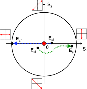
Figure 7: (Color online) Different types of transitions from non-lasing to lasing state in the space of Stokes parameters ($S_{1}$, $S_{2}$): Abrupt transition (blue straight dashed arrow from ${\mathrm{\mathbf{E}}}_{ai}$ to ${\mathrm{\mathbf{E}}}_{af}$, corresponds to device #1) and smooth transition (green curved dashed arrow from ${\mathrm{\mathbf{E}}}_{si}$ to ${\mathrm{\mathbf{E}}}_{sf}$, corresponds to device #2). The initial polarization state for the abrupt transition ${\mathrm{\mathbf{E}}}_{ai}$ is orthogonally polarized to the final one ${\mathrm{\mathbf{E}}}_{af}$, whereas for the initial ${\mathrm{\mathbf{E}}}_{si}$ and final ${\mathrm{\mathbf{E}}}_{sf}$ states for the smooth transition this is not the case. For convenience, the polarizations directions for different quadrants of ($S_{1}$, $S_{2}$)-plane are shown by red arrows in the black boxes. The red cross in the center corresponds to a fully unpolarized state ($p=0$) whereas the black circle shows the fully polarized state ($p=1$).

We will refer to the first case as an “abrupt” transition, and to the second case as a “smooth” one. One can see a remote analogy to the Ising and Bloch transitions Coullet et al. (1990), which also represent abrupt “switching” or smooth “rotating” behavior. The role of the vector of magnetization in this case is played by the Stokes parameters. One should note however that Ising and Bloch transitions occur in space, i.e., between energetically equivalent spatially separated states (at constant external parameters), whereas here the transition takes place in dependence on an external parameter (current), i.e. in the parameter space.

The above mentioned difference between the abrupt and smooth transitions can be expressed more directly in terms of the coherence matrix. For the abrupt transition the coherence matrix is diagonal in one and the same coordinate basis during the whole transition. Only two polarization directions are possible, depending on which diagonal element $J_{11}$ or $J_{22}$ is larger. The point representing the polarization state in Fig.8 can move only along a straight line passing through zero $(S_{1}=0,S_{2}=0)$. At the point of transition $J_{11}=J_{22}$, i.e. the light is unpolarized, and the polarization direction changes abruptly. In the case of a smooth transition the situation is different. Of course, the coherence matrix is Hermitian and therefore there is always a Cartesian coordinate basis in which it is diagonal. However, this basis is changing during the transition. That reflects the existence of several competing mechanisms (DBRs, side boundaries, intra-cavity anisotropies), each of them having its own principal axes. Their mutual influence is changing with a chance of parameter (here current). In this case, the Stokes parameters do not vary along a straight line and can avoid the zero crossing. It should be noted also that the origin $(S_{1}=0,S_{2}=0)$ is a special point in the sense that the coherence matrix in this point is proportional to the identity matrix and therefore is diagonal in every coordinate basis.

IV.4 Detailed discussion

The polarization, intensity and fractional polarization obtained from Eq. (10), Eq. (9) and Eq. (12) are shown in Fig. 4, 5, and 6 in comparison to experimental data. The parameters of the active layer and the cavity used for calculations are $\alpha=3$, $\gamma=10^{3}$ ns^-1, $\gamma_{a}=0.8$ ns^-1, $\gamma_{p}=0$. The DBRs, consisting of 31 (top mirror) and 47 (bottom mirror) $\lambda/4$ layers of material with alternating refractive index $n_{1}=3.46$, $n_{2}=3.093$ and the transparency current $J_{tr}=7$ mA were assumed. The effective round-trip time $\tau=33$ fs includes also the effects of the dispersion in the DBRs and in the cavity Schulz-Ruhtenberg et al. (2005). The outcoupling loses for these parameters are $\kappa_{\mathrm{out}}=17.4$ ns^-1. The best coincidence with the experimental results appears for $\kappa_{\mathrm{in}}=65$ ns^-1, which is in rather good agreement with estimations based on losses in the p-DBR and typical gain values of GaAs quantum wells Babic et al. (1997); Coldren and Corzine (1995).

In the framework of the theory presented here only an infinite device can be considered. Therefore, the final lasing state satisfies always the “90-degree rule” Loiko and Babushkin (2001a). As the laser approaches threshold, the influence of the side boundaries start to play an important role Babushkin et al. (2008), and the polarization may not be perpendicular to ${\mathrm{\mathbf{k}}}_{\bot}$ anymore. For the device #1 this deviation is very small but it is not negligible anymore for the device #2. We take this into account in our model by introducing an artificial rotation of the main axes of the matrix $\Theta$ for the device #2, so it is becomes diagonal not in the basis of s- and p-waves but in another, rotated one. On the other hand, we keep the transition matrix $T$ the same (i. e. diagonal in the basis of s- and p-waves). This makes the resulting coherence matrix non-diagonal. The angle of rotation is 25^∘, which corresponds approximately to the angle of the wavevectors visible in the inset of Fig. 3(a).

Although the spontaneous emission factor is rather small ($\beta_{sp}\approx 10^{-5}$) for VCSELs with a transverse size around 40 $\mu$m Shin et al. (1997), it can be significantly enhanced by the Petermann excess factor. The value of $K$ depends extremely strongly on the inhomogeneities and imperfections in the construction of a particular device. The best results in comparison to experiment give the values $K\beta_{sp}=6\times 10^{-4}$ for the device #1 and $K\beta_{sp}=10^{-2}$ for #2. In Babushkin et al. (2008) it is shown that the four spots at the corners of a rectangular which form the dominant Fourier peaks of the spatial structures (see inset of Fig. 6(a)) can form the eigenmode of the transverse waveguide but are not simultaneously an eigenmode of the reflection operator of the DBR. Thus the reflection couples many transverse wavevectors ${\mathrm{\mathbf{k}}}_{\bot}$. This may be the the origin of the rather large Petermann factor $K$, especially for device #2. In addition, non-orthogonality of the modes might originate from inhomogeneities of the structure and current distribution (which is clearly visible in the intensity distributions in Fig. 2(a-c), Fig. 3(a-c), for both device #1 and #2).

With this choice of parameters, a very good agreement between experiment and theory is obtained for the development of the fractional polarization and the local polarization direction versus current for both devices (Figs. 5, and 6) as well as for the dependence on the transverse wave vector (Fig. 4). The data reflect the degree of abruptness of the transition (Fig. 5c vs. Fig. 6c) and the monotonous vs. non-monotonous development of fractional polarization (Fig. 6b vs. Fig. 5b). The increase of fractional polarization and the convergence towards the “90${}^{\circ}-$rule” with increasing wave number is due to the increasing anisotropy between s- and p-waves, of course (see the blue line in Fig. 8a).

The case of the abrupt transition allows more analytical insight. Let us suppose for the sake of clarity that the isotropic intra-cavity anisotropy is diagonal in the representation of s- and p-waves. In this situation, all the matrices in Eq. (9) and Eq. (10) are diagonal in this representation. Therefore the coherence matrices $J$, $J_{o}$ are also always diagonal. In this case Eq. (9) and Eq. (10) are decoupled into independent equations for the diagonal elements:

$$J_{ii}=\frac{K\beta_{sp}j}{2T_{1}\{\kappa_{\mathrm{in}}+\kappa_{\mathrm{out}}\mathrm{Re}(\Upsilon_{ii})+\mathrm{Re}(\Gamma_{ii})+\kappa_{\mathrm{out}}\langle I\rangle\mathrm{Re}({\cal G}_{ii})\}},\,$$

$$J_{oii}=|T_{ii}|^{2}J_{ii},$$ (13)

where $i=1$ corresponds to the DBR s-wave whereas $i=2$ to the p-wave.

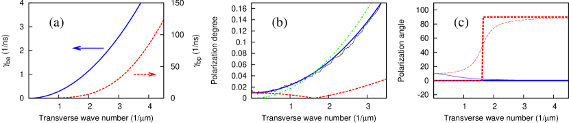
Figure 8: (Color online) (a) The amplitude $\gamma_{ba}$ (blue, solid line) and phase $\gamma_{bp}$ (red, dashed line) anisotropy induced by the Bragg reflector. (b) The degree of polarization for the parameters of device #1 (see Fig. 4) and $k_{y}=0$ according to theoretical calculations. The polarization degree inside the cavity is indicated by the red dashed line, outside the cavity by the blue solid line. The corresponding experimental curve is depicted by the black line. The extra-cavity polarization in the “pure filtering limit” (i.e. assuming completely unpolarized light inside the cavity) is indicated by the green dot-dashed line. (c) The polarization direction inside (red dashed lines) and outside (blue solid lines) the cavity for the intra-cavity anisotropy favoring $x$-polarization (thick lines, as in panel b) or an anisotropy favoring a polarization direction of 10^∘ (thin lines).

Well below threshold the denominator in Eq. (13) is positive and approximately the same for both s- and p- waves (as it will be discussed below), and the light outside of the cavity is slightly p-polarized ($J_{o11}<J_{o22}$) due to the filtering by the Bragg reflector. As the current approaches threshold the denominator for the s-wave in Eq. (13) tends to zero whereas the one for the p-wave remains positive, which provides superiority for the s-wave strongly overcoming the opposite difference in transmission. Obviously, at some point the transition between s- and p-polarization occurs. At the point of transition $J_{o11}=J_{o22}$ (and therefore $S_{1}=0$, $S_{2}=0$), i.e., the output is unpolarized (see Fig. 7, blue straight arrow, and Fig. 5(b)). Because the coherence matrix is diagonal, the polarization direction can have only two values, corresponding to either $J_{o11}<J_{o22}$ (“0-degree rule”) or $J_{o11}>J_{o22}$ (“90-degree rule”). Therefore, at the transition point, the polarization direction changes abruptly and is constant in all other points above and below threshold (see Fig. 5(c)).

Let us now consider the behavior of the extracavity polarization far below threshold (when the intensity-dependent term in Eq. (13) can be neglected). If we suppose that the intra-cavity losses $\kappa_{\mathrm{in}}$ are much larger than the ones through outcoupling $\kappa_{\mathrm{out}}$ and than the intracavity anisotropy $\Gamma_{ii}$ we obtain:

$$J_{ii}=\frac{K\beta_{sp}j}{2T_{1}\kappa_{\mathrm{in}}},\,J_{oii}=|T_{ii}|^{2}J_{ii}.$$ (14)

In this case the output polarization is governed by the transmission through the DBR $|T_{ii}|^{2}$, and the laser cavity works as a simple filter for almost unpolarized intra-cavity radiation. Because $|T_{s}|^{2}>|T_{p}|^{2}$, this results in the “0-degree rule” due to the dominance of p-polarization direction in transmission. In this case (we will call it “pure filtering case” here), the degree of polarization is determined only by the transmitting properties of the Bragg reflector (see Fig. 8(b), green line). The difference in transmission between s- and p-waves increases with $k_{\bot}$ approximately quadratically, and the degree of polarization in this case reflects this dependence according to Eq. (14).

For the opposite case $\kappa_{\mathrm{out}}\gg\kappa_{\mathrm{in}}$ and assuming a diagonal coherence matrix, we obtain

$$J_{oii}\sim|T_{ii}|^{2}/\mathrm{Re}(\Upsilon_{ii}),$$ (15)

instead of Eq. (14). Because for small current $\Upsilon_{ii}\sim 1-|R_{ii}|^{2}=|T_{ii}|^{2}$, the light outside the cavity is completely unpolarized in this case. This is in agreement with the energy conservation principle, since the numbers of intracavity photons in both polarizations are increased by the spontaneous emission equally and the polarizations do not mix. Therefore, in the stationary case in the absence of intracavity losses the energy escaping the cavity must be also equal for both polarizations.

In general, the extracavity polarization degree, defined by Eq. (13), lies in between these two limiting cases (Fig. 8(b), thick, solid blue line). As the Bragg reflection is isotropic for $k_{\bot}=0$ ($\Upsilon_{ii}\left.\right|_{{\mathrm{\mathbf{k}}}_{\bot}=0}=1$ for $i=1,2$), the polarization for ${\mathrm{\mathbf{k}}}_{\bot}\approx 0$ is defined only by the intra-cavity amplitude anisotropy $\gamma_{a}$ (and does not depend on $\gamma_{p}$). The best agreement with the experimental value of the degree of polarization for ${\mathrm{\mathbf{k}}}_{\bot}=0$ is achieved for $\gamma_{a}=0.8$ ns^-1, a reasonable number in line with typical observations in small-area VCSELs van Exter et al. (1998); Sondermann et al. (2004). With increasing transverse wavenumber $k_{\bot}$, the relative importance of the anisotropy induced by $\Upsilon({\mathrm{\mathbf{k}}}_{\bot})$ increases. The amplitude anisotropy $\gamma_{ba}({\mathrm{\mathbf{k}}}_{\bot})=\kappa_{\mathrm{out}}(\mathrm{Re}(\Upsilon_{11}({\mathrm{\mathbf{k}}}_{\bot}))-\mathrm{Re}(\Upsilon_{22}({\mathrm{\mathbf{k}}}_{\bot})))/2$ and the phase anisotropy $\gamma_{bp}({\mathrm{\mathbf{k}}}_{\bot})=\kappa_{\mathrm{out}}(\mathrm{Im}(\Upsilon_{11}({\mathrm{\mathbf{k}}}_{\bot}))-\mathrm{Im}(\Upsilon_{22}({\mathrm{\mathbf{k}}}_{\bot})))/2$, induced by $\Upsilon({\mathrm{\mathbf{k}}}_{\bot})$ are shown in Fig. 8(a). In analogy to the intra-cavity anisotropy, only $\gamma_{ba}$ plays a role in the determining of the coherence matrix. As one can see, $\gamma_{ba}$ increases approximately quadratically with $k_{\bot}$. The degree of polarization inside the cavity (see Fig. 8(b), thick, dashed red line) is influenced more strongly by the intracavity anisotropy for small $k_{\bot}$ (below $\sim 1.5$ $\mu$m^-1) and by the Bragg-induced anisotropy for larger $k_{\bot}$. But it remains relatively small for all $k_{\bot}$, and the polarization degree outside of the cavity is therfore quite strongly determined by the Bragg filtering mechanism (see Fig. 8(b), thick, solid blue line).

Now, let us consider the behavior of the polarization of intra-cavity field in dependence on ${\mathrm{\mathbf{k}}}_{\bot}$ far below threshold in more detail. As an example, a cut displaying the polarization angle along the $k_{x}$ axis, assuming the anisotropy also being directed along the $x$-axis is shown in Fig. Fig. 8(c). In this case, the intracavity and extracavity light for $k_{\bot}\approx 0$ is x-polarized. However, for high enough $k_{\bot}$ (above $\sim 1.5$ $\mu$m^-1) the DBR-induced anisotropy overcomes the intracavity one and the intra-cavity light becomes weakly polarized in the direction perpendicular to ${\mathrm{\mathbf{k}}}_{\bot}$ (see Fig. 8(c), thick red, dashed line). This degree of polarization is small and canceled when the light is transmitted through the Bragg reflector. Hence the polarization of the light outside of the cavity is still determined by the transmission, i.e., is parallel to ${\mathrm{\mathbf{k}}}_{\bot}$, as it mentioned above (see Fig. 8(c), blue lines).

Hence, we also encounter a polarization transition in the intracavity field, if we consider $k_{\bot}$ as a parameter instead of the current. This transition is abrupt (see Fig. 8(c), thick red, dashed line) and the fractional polarization vanishes at the transition point (see Fig. 8(b), thin red, dashed line). It can be understood in a way fully analogous to the abrupt transition appearing with the change of current. It should be noted, that this transition is not apparent outside the cavity (thick blue line in Fig. 8(c)).

This behavior becomes slightly more complex, if one analyzes the polarization along a cut in Fourier space whose direction does not coincide with the preferred intra-cavity anisotropy axis. In that case, the change of polarization angle vs. wavenumber is smooth (Fig. 8(c), thin red line) and also detectable outside the cavity (Fig. 8(c), thin blue line). This is backed up by the experimental curves displayed in Fig. 4a, where the transition is most notable for the cyan curve, which corresponds to a cut along 90^∘; i.e., the competition between intra-cavity anisotropy and Bragg anisotropy is more apparent in the extra-cavity polarization, if the deviation between wavevector and anisotropy angle increases.

V Conclusion

For highly divergent emission in wide aperture VCSELs the polarization direction is determined by the properties of the distributed Bragg reflectors (DBRs), and (close to threshold) by the transverse structure of the cavity. Far below threshold the polarization is independent from the cavity structure and the p-wave of the DBRs (which has the polarization direction parallel to ${\mathrm{\mathbf{k}}}_{\bot}$) prevails in the emission because the almost unpolarized intra-cavity light is filtered by the transmission through the DBR, which is higher for p-waves than for s-waves. In the simplest case, when the above threshold polarization direction is not strongly influenced by the transverse boundaries, an abrupt switch of polarization direction occurs as the current increases towards the laser threshold: the s-wave inside the cavity start to prevail because the reflectivity and therefore the quality factor of the cavity is higher compared to the one for p-wave. At the point of transition the filtering effect of the transmission through the DBR can not compensate the intra-cavity polarization anymore, and the polarization changes its direction from the one parallel to ${\mathrm{\mathbf{k}}}_{\bot}$ to the perpendicular one. This abrupt change of polarization direction is accomplished by the passing through zero of the degree of polarization of the light outside of the cavity.

On the other hand, if the above-threshold polarization does not coincide with the DBR s-mode, the transition is qualitatively different. In this case, the polarization changes smoothly and the degree of polarization is significantly nonzero during all the transition. As was shown in Babushkin et al. (2008), the deviation of the above-threshold polarization direction from the one dictated by the s-wave of the DBRs can be due to the influence of the side boundaries of the cavity.

The difference between two types of transition can be explained in the terms of coherence matrix. The abrupt transition occurs when the coherence matrix of the light outside the cavity is diagonal (in one and the same basis) during the whole transition. In this case, only two polarization directions are possible. If the different mechanisms influencing the polarization have different directions, the resulting coherence matrix is non-diagonal and arbitrary polarization direction is possible.

We note an analogy between the abrupt and smooth transitions described here to Ising and Bloch transitions between two equivalent states in ferromagnetics with respect to a “switching” vs. “rotation” behavior. However, the polarization transition in this article occurs in parameter space (between energetically inequivalent states) in contrast to the usual Bloch and Ising ones.

Appendix A The Ginsburg-Landau equation

A.1 The initial equations

Polarization phenomena in VCSEL are often modeled using an equations for the intracavity field ${\mathrm{\mathbf{E}}}$ and the total carrier density $D$ as well as the population difference $d$ between sub-bands with opposite carrier spin Miguel et al. (1995); Loiko and Babushkin (2001a). We start from the nonlinear equations (18) of Loiko and Babushkin (2001a) for the normalized complex-valued envelope ${\mathrm{\mathbf{E}}}(t,{\mathrm{\mathbf{k}}}_{\bot})$, of the optical field for given ${\mathrm{\mathbf{k}}}_{\bot}$ and carrier population variables $D$, $d$:

$$\dot{{\mathrm{\mathbf{E}}}} = -\kappa_{\mathrm{out}}M{\mathrm{\mathbf{E}}}-i\Omega{\mathrm{\mathbf{E}}}-i\kappa_{\mathrm{out}}\alpha{\mathrm{\mathbf{E}}}+\kappa_{\mathrm{out}}(1+i\alpha)G(A{\mathrm{\mathbf{E}}})+{\mathrm{\mathbf{W}}},$$ (16)

$$\dot{D} = -\gamma_{1}\left\{D-j+\mathrm{Im}\left[(i-\alpha){\mathrm{\mathbf{E}}}^{\ast}{\cal L}(A{\mathrm{\mathbf{E}}})\right]\right\},$$ (17)

$$\dot{d} = -\gamma_{s}d-\gamma_{1}\mathrm{Re}\left[(i-\alpha){\mathrm{\mathbf{E}}}^{\ast}{\cal L}(A{\mathrm{\mathbf{E}}}^{\prime})\right].$$ (18)

Here $\alpha$ is the line width enhancement factor, $j$ is the normalized current density, $\kappa_{\mathrm{out}}$ is the outcoupling losses (see below),$\gamma_{1}=1/T_{1}$ and $\gamma_{s}$ are the decay rates of $D$ and $d$, ${\mathrm{\mathbf{E}}}^{\prime}=\{E_{y},-E_{x}\}$ and $A=\bigl{(}\begin{smallmatrix}D&id\\ -id&D\end{smallmatrix}\bigr{)}$. The linear operators $M({\mathrm{\mathbf{k}}}_{\bot})$, $\Omega({\mathrm{\mathbf{k}}}_{\bot})$, $G({\mathrm{\mathbf{k}}}_{\bot})$, ${\cal L}({\mathrm{\mathbf{k}}}_{\bot})$ describe the losses, diffraction and gain in the cavity, and are $2\times 2$ ${\mathrm{\mathbf{k}}}_{\bot}$-dependent matrices acting on the vector field ${\mathrm{\mathbf{E}}}({\mathrm{\mathbf{k}}}_{\bot})$.

In the present paper we assume that $\Omega({\mathrm{\mathbf{k}}}_{\bot})=-k_{\bot}^{2}v/k_{0}\mathbb{1}+\left(s_{1}({\mathrm{\mathbf{k}}}_{\bot})+s_{2}({\mathrm{\mathbf{k}}}_{\bot})\right)/\tau$ is a matrix describing the dispersion relation given by the cavity resonance condition for s- and p- waves of DBR. Here $v$ is the speed of light in the cavity, $k_{0}$ is the longitudinal part of the wavevector, $\tau$ is the cavity round-trip time, $\mathbb{1}=\mathrm{diag}\,(1,1)$ ($\mathrm{diag}\,(\cdot,\cdot)$ is here a diagonal matrix with corresponding entities on the diagonals), and $s_{1},\,s_{2}$ are the matrices, describing diffraction of the light in the DBRs. In s-p-representation they can be written as $s_{i}=\mathrm{diag}\,(s_{si},s_{pi})$, where $i=1,2$ and $s_{si}$,$s_{pi}$ are the phase shift for s- and p-waves.

Using these assumptions, $M({\mathrm{\mathbf{k}}}_{\bot})$ and $G({\mathrm{\mathbf{k}}}_{\bot})$ can be written in terms of propagation matrices $F_{1}({\mathrm{\mathbf{k}}}_{\bot})=(\rho\tilde{\Gamma})^{1/2}R_{1}({\mathrm{\mathbf{k}}}_{\bot})\exp(-is_{1}({\mathrm{\mathbf{k}}}_{\bot}))$, $F_{2}({\mathrm{\mathbf{k}}}_{\bot})=(\rho\tilde{\Gamma})^{1/2}R_{2}({\mathrm{\mathbf{k}}}_{\bot})\exp(-is_{2}({\mathrm{\mathbf{k}}}_{\bot}))$, $F=F_{1}F_{2}$: $M({\mathrm{\mathbf{k}}}_{\bot})=\left(1-F({\mathrm{\mathbf{k}}}_{\bot})\right)/M_{0},G({\mathrm{\mathbf{k}}}_{\bot})=\left(1+F_{1}({\mathrm{\mathbf{k}}}_{\bot})+F_{2}({\mathrm{\mathbf{k}}}_{\bot})+F({\mathrm{\mathbf{k}}}_{\bot})\right){\cal L}_{\Omega}/G_{0}$. $M$ and $G$ are normalized by the constants $M_{0}$ and $G_{0}$ in such a way, that $M_{11}(0)=1$, $G_{11}(0)=1$. Here $R({\mathrm{\mathbf{k}}}_{t})$ is an operator describing the reflection from the Bragg mirrors, represented by matrices $R_{m}={R_{mij}}\,(m=1,2,i=1,2,\,j=2,2)$. $\kappa_{\mathrm{out}}=(1-|R_{111}(0)||R_{211}(0)|)/\tau=(1-|R_{122}(0)||R_{222}(0)|)/\tau$ is the outcoupling losses for zero transverse mode. $\rho$ describes all intracavity losses in the whole system (which are not due to outcoupling) and $\tilde{\Gamma}$ is the intracavity anisotropy matrix, which in the basis of the main anisotropy axes is written as

$$\tilde{\Gamma}=\left(\begin{smallmatrix}\exp(\gamma_{a}\tau+i\gamma_{p}\tau)&0\\ 0&\exp(-\gamma_{a}\tau-i\gamma_{p}\tau)\\ \end{smallmatrix}\right)$$ (19)

where $\gamma_{a}$ is the amplitude anisotropy and $\gamma_{p}$ is the birefringence. The influence of the gain contour line ${\cal L}({\mathrm{\mathbf{k}}}_{\bot})$ is given by the expression ${\cal L}=1/\left(1+((\delta-\Omega)/\gamma)^{2}\right)$ where $L$ is the cavity length and $\gamma$ is the material polarization decay rate.

The spontaneous emission is described by the term ${\mathrm{\mathbf{W}}}=\sqrt{K\beta_{sp}\gamma_{1}D}\boldsymbol{\xi}$ in the approximation of zero inter-sub-band population difference. Here, $K$ is the Petermann excess quantum noise factor and $\beta_{sp}$ is the spontaneous emission factor. $\boldsymbol{\xi}$ is the Langevin noise source with zero mean and correlation in $(x,y)$-space and circular wave basis $\boldsymbol{\xi}(x,y,t)=\{\xi_{+}(x,y,t),\xi_{-}(x,y,t)\}$:

$$\langle\xi_{\pm}(x,y,t)\xi_{\pm}(x^{\prime},y^{\prime},t^{\prime})\rangle=2\delta(t-t^{\prime})\delta(x-x^{\prime})\delta(y-y^{\prime}),\,$$

$$\langle\xi_{\pm}(x,y,t)\xi_{\mp}(x^{\prime},y^{\prime},t^{\prime})\rangle=0.$$ (20)

Performing the transverse Fourier transform and transforming into a basis of linear (orthonormal) polarization with arbitrary directions of the axes $1$ and $2$ one obtains the analogous equation for $\boldsymbol{\xi}(k_{x},k_{y},t)=\{\xi_{1}(k_{x},k_{y},t),\xi_{2}(k_{x},k_{y},t)\}$:

$$\begin{split}\langle\xi_{j}(k_{x},k_{y},t)\xi_{i}(k^{\prime}_{x},k^{\prime}_{y},t^{\prime})\rangle=2\delta_{ij}\delta(t-t^{\prime})\times\\ \times\delta(k_{x}-k_{x}^{\prime})\delta(k_{y}-k_{y}^{\prime}).\end{split}$$ (21)

Therefore, the noise is also correlated in the ${\mathrm{\mathbf{k}}}_{\bot}$-representation and in an arbitrary orthogonal polarization basis. The noise terms in the equations for $D$ and $d$ are neglected in the present consideration.

A.2 The derivation of the Ginsburg-Landau equation (GLE) for the field

Here we obtain the lowest-order nonlinear equations for the field resulting from the above mentioned nonlinear equations. We take into account that near lasing threshold the resulting linear operator acting on ${\mathrm{\mathbf{E}}}$, $D$, $d$ has a block-diagonal form with the part acting on ${\mathrm{\mathbf{E}}}$ not being coupled to the carrier part. The eigenvalues stemming from the carrier related part are always strongly negative. In addition, the solution with $d=0$ is always possible. Then, it is possible to adiabatically eliminate $D$ and obtain a complex equation for ${\mathrm{\mathbf{E}}}$ only.

The solution of $\dot{D}=0$ is given then by $D=j/(1+I{\cal L})$, where $I=|{\mathrm{\mathbf{E}}}|^{2}$. For small intensity $I$ one can write it as $D\sim j(1-I{\cal L})$. Substituting this into the equation for the field, we obtain:

$$\begin{split}\dot{{\mathrm{\mathbf{E}}}}=-\kappa_{\mathrm{out}}M{\mathrm{\mathbf{E}}}-i\Omega{\mathrm{\mathbf{E}}}-i\kappa_{\mathrm{out}}\alpha{\mathrm{\mathbf{E}}}+\kappa_{\mathrm{out}}(1+i\alpha)jG{\cal L}{\mathrm{\mathbf{E}}}-\\ -\kappa_{\mathrm{out}}(1+i\alpha)jG{\cal L}^{2}I{\mathrm{\mathbf{E}}}+{\mathrm{\mathbf{W}}}.\end{split}$$ (22)

Because the anisotropy and the intracavity losses are small compared to $1$, the corresponding terms can be decomposed as $\rho=\exp(-\kappa_{\mathrm{in}}\tau)\approx 1-\kappa_{\mathrm{in}}\tau$, $\tilde{\Gamma}\approx 1+\Gamma\tau$ with $\Gamma=\mathrm{diag}\,(\gamma_{a}+i\gamma_{p},-\gamma_{a}-i\gamma_{p})$. Considering $\kappa_{\mathrm{in}}\tau$, $\kappa_{\mathrm{out}}\tau$ and $\Gamma\tau$ as small parameters and neglecting these terms starting from the first order in $G$ and from the second order in $M$, and introducing the matrices ${\cal G}=(1+i\alpha)j\tilde{G}{\cal L}^{2}$, $\Upsilon=\tilde{M}+i\alpha-(1+i\alpha)j\tilde{G}{\cal L}$ (where $\tilde{M}=M\left|{}_{\rho=1,\tilde{\Gamma}=1}\right.$, $\tilde{G}=G\left|{}_{\rho=1,\tilde{\Gamma}=1}\right.$) we obtain the resulting GLE (4).

The spontaneous emission term in the approximation of a small intensity can be written as ${\mathrm{\mathbf{W}}}({\mathrm{\mathbf{k}}}_{\bot},t)=\sqrt{K\beta_{sp}\gamma_{1}j}\boldsymbol{\xi}({\mathrm{\mathbf{k}}}_{\bot},t)$. Here we neglected the second order term in decomposition of stationary value of $D$ into series.

References

- Wilmsen et al. (1999) C. Wilmsen, H. Temkin, and L. A. Coldren, Vertical-cavity surface-emitting lasers (Cambridge University Press, Cambridge, 1999).
- Mulet et al. (2001) J. Mulet, C. Mirasso, and M. San Miguel, Phys. Rev. A 64, 023817 (2001).
- Hermier et al. (2002) J.-P. Hermier, M. I. Kolobov, I. Maurin, and E. Giacobino, Phys. Rev. A 65, 053825 (2002).
- Willemsen et al. (2001) M. B. Willemsen, A. S. v. d. Nes, M. P. v. Exter, J. P. Woerdman, M. Kicherer, R. King, R. Jäger, and K. J. Ebeling, J. Appl. Phys. 89, 4183 (2001).
- Shelly et al. (2000) D. Shelly, T. Garrison, M. K. Beck, and D. Christensen, Opt. Exp. 7, 249 (2000).
- Golubev et al. (2004) Y. M. Golubev, T. Y. Golubeva, M. I. Kolobov, and E. Giacobino, Phys. Rev. A 70, 053817 (2004).
- Miguel et al. (1995) M. S. Miguel, Q. Feng, and J. V. Moloney, Phys. Rev. A 52, 1728 (1995).
- Travagnin et al. (1996) M. Travagnin, M. P. v. Exter, A. K. Jansen, A. K. J. v. Doorn, and J. P. Woerdman, Phys. Rev. A 54, 1647 (1996).
- Travagnin (1997) M. Travagnin, Phys. Rev. A 56, 4094 (1997).
- Sondermann et al. (2003) M. Sondermann, M. Weinkath, T. Ackemann, J. Mulet, and S. Balle, Phys. Rev. A 68, 033822 (2003).
- Balle et al. (1999) S. Balle, E. Tolkacheva, M. S. Miguel, J. R. Tredicce, J. Martín-Regalado, and A. Gahl, Opt. Lett. 24, 1121 (1999).
- Panajotov et al. (2000) K. Panajotov, B. Nagler, G. Verschaffelt, A. Georgievski, H. Thienpont, J. Danckaert, and I. Veretennicoff, Appl. Phys. Lett. 77, 1590 (2000).
- Ptashchenko (1996) Ptashchenko, Solid State Electronics 39, 1495 (1996).
- Moloney and Newel (1990) J. V. Moloney and A. C. Newel, Physica D 44, 1 (1990).
- Jakobsen et al. (1992) P. K. Jakobsen, J. V. Moloney, A. C. Newell, and R. Indik, Phys. Rev. A 45, 8129 (1992).
- Hegarty et al. (1999a) S. Hegarty, G. Huyet, J. G. McInerney, and K. D. Choquette, Phys. Rev. Lett. 82, 1434 (1999a).
- Loiko and Babushkin (2001a) N. A. Loiko and I. V. Babushkin, J. Opt. B: Quantum Semiclass. Opt. 3, S234 (2001a).
- Babushkin et al. (2008) I. Babushkin, M. Schulz-Ruhtenberg, N. A. Loiko, K. F. Huang, and T. Ackemann, Phys. Rev. Lett. 100, 213901 (2008).
- Schulz-Ruhtenberg et al. (2009) M. Schulz-Ruhtenberg, Y. Tanguy, R. Jäger, and T. Ackemann, Appl. Phys. B (2009); DOI 10.1007/s00340-009-3718-2.
- Hegarty et al. (1999b) S. P. Hegarty, G. Huyet, P. Porta, J. G. McInerney, K. D. Choquette, K. M. Geib, and H. Q. Hou, J. Opt. Soc. Am. B 16, 2060 (1999b).
- Schulz-Ruhtenberg et al. (2005) M. Schulz-Ruhtenberg, I. Babushkin, N. A. Loiko, T. Ackemann, and K. F. Huang, Appl. Phys. B 81, 945 (2005).
- Loiko and Babushkin (2001b) N. A. Loiko and I. V. Babushkin, Quantum Electronics 31, 221 (2001b).
- Babushkin et al. (2004) I. V. Babushkin, N. A. Loiko, and T. Ackemann, Phys. Rev. E 69, 066205 (2004).
- Born and Wolf (1980) M. Born and E. Wolf, Principles of Optics (Pergamon, Oxford, 1980).
- Babic et al. (1993) D. I. Babic, Y. Chung, N. Dagli, and J. E. Bowers, IEEE J. Quantum Electron. 29, 1950 (1993).
- Petermann (1979) K. Petermann, IEEE J. Quantum Electron. 15, 566 (1979).
- Gardiner (2004) C. W. Gardiner, Handbook of Stochastic Methods for Physics, Chemistry, and the Natural Sciences (Springer, New York, 2004).
- Mandel and Wolf (1995) L. Mandel and E. Wolf, Optical Coherence and Quantum Optics (Cambridge University Press, Cambridge, New York; Australia, 1995).
- Giacomelli and Marin (1998) G. Giacomelli and F. Marin, Quantum Semiclass. Opt. 10, 469 (1998).
- Coullet et al. (1990) P. Coullet, J. Lega, B. Houchmanzadeh, and J. Lajzerowics, Phys. Rev. Lett. 65, 1352 (1990).
- Babic et al. (1997) D. I. Babic, J. Piprek, K. Streubel, R. P. Mirin, N. M. Margalit, D. E. Mars, J. E. Bowers, and E. L. Hu, IEEE J. Quantum Electron. 33, 1369 (1997).
- Coldren and Corzine (1995) L. A. Coldren and S. W. Corzine, Diode Lasers and Photonic Integrated Circuits (Wiley, New York, 1995).
- Shin et al. (1997) J. H. Shin, H. E. Shin, and Y. H. Lee, Appl. Phys. Lett. 70, 2652 (1997).
- van Exter et al. (1998) M. P. van Exter, A. Al-Remawi, and J. P. Woerdman, Phys. Rev. Lett. 80, 4875 (1998).
- Sondermann et al. (2004) M. Sondermann, M. Weinkath, and T. Ackemann, IEEE J. Quantum Electron. 40, 97 (2004).