RANDOM SCATTERING OF BITS BY PREDICTION

Abstract.

We investigate a population of binary mistake sequences that result from learning with parametric models of different order. We obtain estimates of their error, algorithmic complexity and divergence from a purely random Bernoulli sequence. We study the relationship of these variables to the learner’s information density parameter which is defined as the ratio between the lengths of the compressed to uncompressed files that contain the learner’s decision rule. The results indicate that good learners have a low information density$\rho$ while bad learners have a high $\rho$. Bad learners generate mistake sequences that are atypically complex or diverge stochastically from a purely random Bernoulli sequence. Good learners generate typically complex sequences with low divergence from Bernoulli sequences and they include mistake sequences generated by the Bayes optimal predictor. Based on the static algorithmic interference model of [18] the learner here acts as a static structure which “scatters” the bits of an input sequence (to be predicted) in proportion to its information density $\rho$ thereby deforming its randomness characteristics.

1. Overview

Ratsaby [18] introduced a quantitative definition of the information content of a general static system (e.g. a solid or some fixed structure) and explained how it algorithmically interferes with input excitations thereby influencing its stability. His model is based on concepts of the theory of algorithmic information and randomness. He modeled a system as a selection rule of a finite algorithmic complexity which acts on an incoming sequence of random external excitations by selecting a subsequence as output. As postulated in [18] a simple structure is one whose information content is small. Its selection behavior is of low complexity since it can be more concisely described. Consequently it is less able to deform properties of randomness of the input sequence. And vice versa, if the system is sufficiently complex it can significantly deform the randomness at the input. Following [18] there have been recent theoretical and empirical results that validate his model for specific problem domains. The first empirical proof of his model appeared in [25, 26, 7] where it was shown that this inverse relationship between system complexity and randomness exists also in a real physical system. The particular system investigated consisted of a one-dimensional vibrating solid-beam to which a random sequence of external input forces is applied. In [19, 21] the problem of learning to predict binary sequences was shown to be an exemplar of this paradigm. The complexity of a learner’s decision rule is proportional to the amount that the subsequence selected by the learner (via his mistakes) deviates from a truly random sequence. A first empirical investigation of this learning problem appeared in [23, 22, 24] where a new measure of system complexity called the sysRatio was introduced and shown to be a proper measure of a learner’s decision complexity.

The current paper digs further along this line and provides not only further empirical analysis and justification of the model of [18] applied to the problem of learning but also gives new interpretations of standard learning phenomena such as model data underfitting or overfitting. It is shown that these phenomena can be interpreted as certain types of deformations of randomness of the binary mistake sequences. These deformations are measured in the $\Delta\ell$-plane ($\Delta$ stands for divergence and $\ell$ for estimated Kolmogorov complexity). We conclude that the prediction rule obtained by learning is analogous to a physical static object that scatters a random beam of particles. We call this phenomena bit-scattering (we discuss this phenomenon later at the end of section 5). The current paper is a further justification that the static algorithmic interference model defined in [18] applies to the problem of learning to predict. Before proceeding to give an introduction to the main concepts let us state the problem that we consider in the paper.

Statement of the problem: Given a random source that generates two binary sequences, $x^{(m)}$ and $x^{(n)}$ of length $m$ and $n$, respectively, according to a finite Markov chain of unknown order $k^{*}$ with an unknown probability transition matrix. A learner uses $x^{(m)}$ to estimate the probability parameters of a Markov model of order $k$. Once the model is learnt, the learner makes a prediction for every bit in $x^{(n)}$. Denote by $y^{(n)}$ the binary sequence corresponding to these predictions. Denote by $\xi^{(n)}$ the error sequence that corresponds to the learner’s predictions where the $i^{th}$ bit $\xi_{i}=1$ if the prediction differs from the true value, i.e., $y_{i}\neq x_{i}$ and $\xi_{i}=0$ otherwise. Denote by $\xi_{0}^{(n)}$ the subsequence of $\xi^{(n)}$ corresponding to those bits of $y^{(n)}$ that are $0$. In this paper we study different characteristics of the error sequence $\xi_{0}^{(n)}$ and how they depend on the two main learner’s parameters, the training sequence length $m$ and the model order $k$. We focus on two main characteristics, the algorithmic complexity of the error sequence and the statistical deviation between the frequency of $1$s and the probability of seeing a $1$ in the sequence. We determine their interrelationship and how the probability of a prediction error depends on them.

The remainder of the paper is organized as follows: in section 2 we introduce the basic concepts of algorithmic complexity and related properties of randomness. In section 3 we review the concept of a selection rule, in section 4 we state a relationship between the complexity of a finite random binary sequence and its entropy. Section 5 describes the experimental setup used for the analysis followed by section 6 which describes the results.

Before continuing, we should clarify at this point that our use of the words ’chaoticity’ or ’chaotic’ is different from chaos theory. By a chaotic binary sequence we do not necessarily mean that it is generated by some dynamical system that is highly sensitive to initial conditions but that it is highly disordered, or in other words, has a high algorithmic complexity.

2. Introduction

Algorithmic randomness (see [6, 12, 5]) is a notion of randomness of an individual element (object) of a sample space. It reflects how chaotic, or how complicated it is to describe the object. Classical probability theory assigns probabilities to sets of outcomes of random trials in an experiment. For instance, consider an experiment with $n$ randomly and independently drawn binary numbers $X_{i}$, $i=1,\ldots n$, where $X_{i}=1$ with probability $\nicefrac{{1}}{{2}}$. Then any outcome such as $X=\left(0,0,\ldots,0\right)$ has the same probability $2^{-n}$. However, from an algorithmic perspective, it is clear that the string $X=\left(0,0,\ldots 0\right)$ is not random compared to some other possible string with a more complicated pattern of zeros and ones. Algorithmic randomness of finite objects (binary sequences) aims to explain the intuitive idea that a sequence, whether finite or infinite, should be measured as being more unpredictable if it possess fewer regularities (patterns). There is no formal definition of randomness but there are three main properties that a random binary string of length $n$ must intuitively satisfy [28]. The first property is the so-called stochasticity or frequency stability of the sequence which means that any binary word of length $k\leq n$ must have the same frequency limit (equal to $2^{-k}$). This is basically the notion of normality that Borel introduced and is related to the degree of unpredictability of the sequence. The second property is chaoticity or disorderliness of the sequence. A sequence is less chaotic (less complex) if it has a short description, i.e., if the minimal length of a program that generates the sequence is short. The third property is typicalness. A random sequence is a typical representative of the class $\Omega$ of all binary sequences. It has no specific features distinguishing it from the rest of the population. An infinite binary sequence is typical if each small subset $E$ of $\Omega$ does not contain it (the correct definition of a ’small’ set was given by Martin L$\ddot{o}$f [16]).

Algorithmic randomness was first considered by von Mises in 1919 who defined an infinite binary sequence $\alpha$ of zeros and ones as random if it is unbiased, i.e. if the frequency of zeros goes to $\nicefrac{{1}}{{2}}$, and every subsequence of $\alpha$ that we can extract using an admissible selection rule (see definition below) is also not biased. Kolmogorov and Loveland [15, 14] proposed a more permissive definition of an admissible selection rule as any (partial) computable process which, having read any $n$ bits of an infinite binary sequence $\alpha$, picks a bit that has not been read yet, decides whether it should be selected or not, and then reads its value. When subsequences selected by such a selection rule pass the unbiasedness test they are called Kolmogorov-Loveland stochastic (KL-stochastic for short). Martin L$\ddot{o}$f [16] introduced a notion of randomness which is now considered by many as the most satisfactory notion of algorithmic randomness. His definition says precisely which infinite binary sequences are random and which are not. The definition is probabilistically convincing in that it requires each random sequence to pass every algorithmically implementable statistical test of randomness.

In this paper we are concerned with random sequences that arise from the process of learning and prediction, or more specifically, from the prediction mistakes made by a learner. Let $X^{(n)}=X_{1},\ldots,X_{n}$ be a sequence of binary random variables drawn according to some unknown joint probability distribution $\mathbb{P}\left(X^{(n)}\right)$. Consider the problem of learning to predict the next bit in a binary sequence drawn according to $\mathbb{P}$. For training, the learner is given a finite sequence $x^{(m)}$ of bits $x_{t}\in\left\{0,1\right\},$ $1\leq t\leq m$, drawn according to $\mathbb{P}$ and estimates a model $\mathcal{M}$ that can be used to predict the next bit of a partially observed sequence. After training, the learner is tested on another sequence $x^{(n)}$ drawn according to the same unknown distribution $\mathbb{P}$. Using $\mathcal{M}$ he produces the bit $y_{t}$ as a prediction for $x_{t}$ , $1\leq t\leq n$. Denote by $\xi^{(n)}$ the corresponding binary sequence of mistakes where $\xi_{t}=1$ if $y_{t}\neq x_{t}$ and is $0$ otherwise. Denote by $\xi_{0}^{(n)}$ the subsequence of $\xi^{(n)}$ that corresponds to the times $t$ where the learner predicted $y_{t}=0$. Note that $\xi_{0}^{(n)}$ is also a subsequence of $x^{(n)}$ so we can view the process of predicting as a process of selecting a subsequence of the input $x^{(n)}$.

It is clear that the subsequence $\xi_{0}^{(n)}$ of mistakes should be random since the test sequence $x^{(n)}$ is random. It is reasonable to expect that the learner may implicitly vary some of the randomness characteristics of the subsequence of bits that he selects thereby cause $\xi_{0}^{(n)}$ to be less random than $x^{(n)}$. In this sense, we may say that the learner ’deforms’ the randomness of the input $x^{(n)}$ producing a less random subsequence of $x^{(n)}$. Or perhaps the learner being of a finite complexity is limited in his ability to ’deform’ randomness of $x^{(n)}$. Essentially we ask what ’interference’ does a learner have on the randomness of a test sequence. It appears essential that we look not only on the randomness of the object itself (the test sequence $x^{(n)}$) but also at the interfering entity—the learner, specifically, its algorithmic component that is used for prediction.

3. Selection rule

Let us formally define a selection rule. This is a principal concept used as part of tests of randomness of sequences (mentioned above). Let $\left\{0,1\right\}^{*}$ be the space of all finite binary sequences and denote by $\left\{0,1\right\}^{n}$ the set of all finite binary sequences of length $n$. An admissible selection rule $R$ is defined [14, 29] based on three partial recursive functions $f,g$ and $h$ on $\left\{0,1\right\}^{*}$. Let $x^{(n)}=x_{1},\ldots,x_{n}$. The process of selection is recursive. It begins with an empty sequence $\emptyset$. The function $f$ is responsible for selecting possible candidate bits of $x^{(n)}$ as elements of the subsequence to be formed. The function $g$ examines the value of these bits and decides whether to include them in the subsequence. Thus $f$ does so according to the following definition: $f(\emptyset)=i_{1}$, and if at the current time $k$ a subsequence has already been selected which consists of elements $x_{i_{1}},\ldots,x_{i_{k}}$ then $f$ computes the index of the next element to be examined according to element $f(x_{i_{1}},\ldots,x_{i_{k}})=i$ where $i\not\in\{i_{1},\ldots,i_{k}\}$, i.e., the next element to be examined must not be one which has already been selected (notice that maybe $i<i_{j}$, $1\leq j\leq k$, i.e., the selection rule can go backwards on $x$). Next, the two-valued function $g$ selects this element $x_{i}$ to be the next element of the constructed subsequence of $x$ if and only if $g(x_{i_{1}},\ldots,x_{i_{k}})=1$. The role of the two-valued function $h$ is to decide when this process must be terminated. This subsequence selection process terminates if $h(x_{i_{1}},\ldots,x_{i_{k}})=1$ or $f(x_{i_{1}},\ldots,x_{i_{k}})>n$. Let $R(x^{(n)})$ denote the selected subsequence. By $K(R|n)$ we mean the length of the shortest program computing the values of $f$, $g$ and $h$ given $n$.

From the above discussion, we know that there are two principal measures related to the information content in a finite sequence $x^{(n)}$, stochasticity (unpredictability) and chaoticity (complexity). An infinitely long binary sequence is regarded random if it satisfies the principle of stability of the frequency of $1$s for any of its subsequences that are obtained by an admissible selection rule [14]. Kolmogorov showed that the stochasticity of a finite binary sequence $x$ may be precisely expressed by the deviation of the frequency of ones from some $0<p<1$, for any subsequence of $x^{(n)}$ selected by an admissible selection rule $R$ of finite complexity $K(R|n)$ where for an object $x$ given another object $y$ he defined in [13] the complexity of $x$ as

$$K(x|y)=\min\{l(\pi):\phi(\pi,y)=x\}$$ (3.1)

where $l(\pi)$ is the length of the sequence $\pi$, $\phi$ is a universal partial recursive function which acts as a description method, i.e., when provided with input $(\pi,y)$ it gives a specification for $x$ (for an introduction see section 2 of [26]). The chaoticity of $x^{(n)}$ is large if its complexity is close to its length $n$. The classical work of [2, 3, 14, 29] relates chaoticity to stochasticity. In [2, 3] it is shown that chaoticity implies stochasticity. For a binary sequence $s$, let us denote by $\|s\|$ the number of $1$s in $s$, then this can be seen from the following relationship (with $p=\nicefrac{{1}}{{2}}$):

$$\left|\frac{\|R(x^{(n)})\|}{l(R(x^{(n)}))}-\frac{1}{2}\right| \leq c\sqrt{\frac{n-K(x^{(n)}|n)+K(R|n)+2\log K(R|n)}{l(R(x^{(n)}))}}$$ (3.2)

where $l(R(x^{(n)}))$ is the length of the subsequence selected by $R$ and $c>0$ is some absolute constant. Apparently as the chaoticity of $x^{(n)}$ grows the stochasticity of the selected subsequence $R(x^{(n)})$ grows (the bias from $\nicefrac{{1}}{{2}}$ decreases). Also, and more relevant to the context of this paper, the information content of the selection rule namely $K(R|n)$ has a direct effect on this relationship: the lower $K(R|n)$ the stronger the stability (smaller deviation of the frequency of $1$s from $\nicefrac{{1}}{{2}}$). In [11] the other direction which shows that stochasticity implies chaoticity is proved.

It was recently shown in [19, 21] that the level of randomness of the subsequence $\xi_{0}^{(n)}$ of $\xi^{(n)}$ which corresponds to the occurrences of mistakes in predicting $0$s decreases relative to an increase in the complexity of the learner. The approach taken there is to represent the learner’s decision as a selection rule that selects $\xi_{0}^{(n)}$ from $\xi^{(n)}$. The rule’s complexity is defined based on a combinatorial quantity rather than Kolmogorov complexity but still yields a relationship of the form of (3.2). This relationship shows that the possibility of deviation of the frequency of $1$s in $\xi_{0}^{(n)}$ from the probability $p_{0}$ of seeing a $1$ in $\xi_{0}^{(n)}$ grows as the complexity of the class of possible decisions grows.

The current paper investigates this experimentally. We consider a learner’s prediction (or decision) rule which we term as system and study its influence on a random binary test sequence on which prediction decisions are made. The system is based on the maximum a posteriori probability decision where probabilities are defined by a statistical parametric model which is estimated from data. The learner of this model is a computer program that trains from a given random data sequence and then produces a decision rule by which it is able to predict (or decide) the value of the next bit in future (yet unseen) random binary sequences. As in [19, 21] we focus on Markov source and a Markov learner whose orders may differ.

4. Relationship to information theory

We now describe the connection between the concepts of entropy (Shannon entropy) and algorithmic complexity. Entropy is a measure of unpredictability of a random variable. Intuitively, we expect that the more unpredictable a sequence of random variables the higher its algorithmic (Kolmogorov) complexity. This is formally expressed as Theorem 14.3.1 in [9] which we now state: denote by $H(X_{1})$ the entropy of a random variable $X_{1}$ and consider a sequence of random variables $\left\{X_{i}\right\}$ drawn i.i.d. according to the probability mass function $f(x)$, $x\in\mathcal{X}$, where $\mathcal{X}$ is a finite alphabet. Let $f(x^{(n)})=\prod_{i=1}^{n}f(x_{i})$. Then there exists a constant $c$ such that

$$H(X_{1})\leq\frac{1}{n}\sum_{x^{(n)}}f(x^{(n)})K(x^{(n)}|n)\leq H(X_{1})+\frac{\left(\left|\mathcal{X}\right|-1\right)\log n}{n}+\frac{c}{n}$$

for all $n$. Consequently, the expected value $E\frac{1}{n}K(X^{(n)}|n)\rightarrow H(X_{1})$ with increasing $n$. This means that the expected value of the Kolmogorov complexity of the sequence converges to the Shannon entropy of the sequence with increasing $n$.

A more relevant estimate for our work here concerns the Kolmogorov complexity of a specific sequence (not the expected value over all sequences). In the case of a Bernoulli random sequence $\left\{X_{i}\right\}_{i=1}^{n}$ with probability $p=P(X_{i}=1)$ its complexity relates to the binary entropy $H(X_{1})$ of any of the i.i.d. random variables of the sequence. It is based on the following statement which holds even more generally for any binary sequence of length $n$ (Theorem 14.2.5 of [9]): Let $x^{(n)}=x_{1},x_{2},\ldots,x_{n}$ be a binary string then the Kolmogorov complexity of $x^{(n)}$ is bounded as

$$K(x^{(n)}|n) \leq nH(p)+\frac{1}{2}\log_{2}n+c$$ (4.1)

where $p=\frac{1}{n}\sum_{i=1}^{n}x_{i}$, $H(p)=-p\log_{2}p-(1-p)\log_{2}(1-p)$ is the entropy of a binary random variable with probability $p$ and $c$ is some finite positive constant independent of $n$ and of the sequence $x^{(n)}$. In particular, we may compute this bound for the random mistake sequences $\xi_{0}^{(n)}$ that we are interested in. In section 6 we use this as a comparison with the empirical estimated algorithmic complexity which is obtained by compression. We proceed to describe the setup.

5. Experimentl setup

The learning problem consists of predicting the next bit in a given sequence generated by a Markov chain (model) $\mathcal{M}^{*}$ of order $k^{*}$. There are $2^{k^{*}}$ states in the model each represented by a word of $k^{*}$ bits. During a learning problem, the source’s model is fixed. A learner, unaware of the source’s model, has a Markov model of order $k$. We denote by $p(1|i)$ the probability of transiting from state $i$ whose binary $k$-word is $b_{i}=[b_{i}(1),\ldots,b_{i}(k)]$ to the state whose word is $[b_{i}(2),\ldots,b_{i}(k),1]$. Given a random sequence of length $m$ generated by the source the learner estimates its own model’s parameters $p(1|i)$ by $\hat{p}(1|i)$, $1\leq i\leq 2^{k}$, which is the frequency of the event “$b_{i}$ is followed by a $1$” in the training sequence. We denote by $\hat{\mathcal{M}}$ the learnt model with parameters $\hat{p}(1|i)$, $1\leq i\leq 2^{k}$. We denote by $p^{*}(1|i)$ the transition probability from state $i$ of the source model, $1\leq i\leq 2^{k}$.

A simulation run is characterized by the parameters, $k$ and $m$. It consists of a training and testing phases. In the training phase we show the learner a binary sequence of length $m$ and he estimates the transition probabilities. In the testing phase we show the learner another random sequence (generated by the same source) of length $n$ and test the learner’s predictions on it. For each bit in the test sequence we record whether the learner has made a mistake. When a mistake occurs we indicate this by a $1$ and when there is no mistake we write a $0$. The resulting sequence of length $n$ is the generalization mistake sequence $\xi^{(n)}$. We denote by $\xi_{0}^{(n)}$ the binary subsequence of $\xi^{(n)}$ that corresponds to the mistakes that occurred only when the learner predicted a $0$. Its length is denoted by $n_{0}$. We denote by $p_{0}$ the probability of mistake when predicting a $0$, i.e., $p_{0}$ is the probability of seeing a $1$ in the subsequence $\xi_{0}^{(n)}$.

For a fixed $k$ denote by $N_{k,m}$ the number of runs with a learner of order $k$ and training sample of size $m$. The experimental setup consists of $N_{k,m}=10$ runs with $1\leq k\leq 10$, $m\in\left\{100,200,\ldots,10000\right\}$ with a total of $100\cdot 10\cdot N_{k,m}=10000$ runs. The testing sequence is of length $n=1000$. Each run results in a file called system which contains a binary vector $d$ whose $i^{th}$ bit represents the maximum a posteriori decision made at state $i$ of the learner’s model, i.e.,

$$d_{i}=\left\{\begin{array}[]{cc}1&\text{if \, }\hat{p}(1|i)>\nicefrac{{1}}{{2}}\\ 0&otherwise\end{array}\right.$$ (5.1)

for $1\leq i\leq 2^{k}$. Let us denote by $\alpha_{i}=P(\hat{p}(1|i)>\nicefrac{{1}}{{2}})$, thus $d_{i}$ are Bernoulli random variables with parameters $\alpha_{i}$, $1\leq i\leq 2^{k}$. The learner’s system is comprised of the decision at every possible state.

Another file generated is the errorT0 which contains the mistake subsequence $\xi_{0}^{(n)}$. At the end of each run we measure the lengths of the system file and its compressed length where compression is obtained either via the Gzip algorithm (a variant of [30]) or the PPM algorithm [8] and compute the sysRatio (denoted as $\rho)$ which is the ratio of the compressed to uncompressed length of the system file. Note that $\rho$ is a measure of information density since it captures the number of bits of useful information (useful for describing the system) per bit of representation (in the uncompressed file).

We do similarly for the mistake-subsequence $\xi_{0}^{(n)}$ obtaining the length $\ell_{0}$ of the compressed file that contains $\xi_{0}^{(n)}$ (henceforth referred to as the estimated algorithmic complexity of $\xi_{0}^{(n)}$ since it is an approximation of the Kolmogorov complexity of $\xi_{0}^{(n)}$, see [26]). We measure the KL-divergence $\Delta_{0}$ between the probability distribution $P(w|\hat{p})$ of binary words $w$ of length $4$ and the empirical probability distribution $\hat{P}_{m}(w)$ as measured from the mistake subsequence $\xi_{0}^{(n)}$. Note, $P(w|\hat{p})$ is defined according to the Bernoulli model with parameter $\hat{p}_{0}$, that is, $P(w|\hat{p}_{0})=\hat{p}_{0}^{i}(1-\hat{p}_{0})^{4-i}$ for a word $w$ with $i$ ones, where $\hat{p}_{0}$ is the frequency of ones in the subsequence $\xi_{0}^{(n)}$. The distribution $\hat{P}_{m}(w)$ equals the frequency of a word $w$ in $\xi_{0}^{(n)}$. Hence $\Delta_{0}$ reflects by how much $\xi_{0}^{(n)}$ deviates from being random according to a Bernoulli sequence with parameter $p_{0}$ (the mistake probability when predicting a $0$).

6. Results

We are interested in determining the relationship between the estimated algorithmic complexity $\ell_{0}$ of $\xi_{0}^{(n)}$, its divergence $\Delta_{0}$ and the learning performance. As the learning performance we look at the generalization error of type $0$ that is the error for $0$-predictions. We choose four different levels of learning problems, controlled by the order of the source model $k^{*}=3$, $4$, $5$, $6$. For each problem we choose for the source model a transition matrix of probabilities $p^{*}(1|i)=1-p$, $p^{*}(0|i)=p$, where for some of the states $i$ we set $p=0.3$ and for others $p=0.7$, $1\leq i\leq 2^{k^{*}}$. Thus the Bayes optimal error is $0.3$. To ensure that the problem is sufficiently challenging we set the first half of the states (those ranging from the $k^{*}$-dimensional vector $00\ldots 0$ to $011\ldots 1$) to have $p=0.3$ and the second half ($10\ldots 0$ to $11\ldots 1$) to have $p=0.7$. This ensures that a Markov model of order $k<k^{*}$ cannot approximate the true transition probabilities well. That is, the infinite-sample limit estimate based on a Markov model of order $k$ which is smaller than $k^{*}$ will still be $\hat{p}(1|i)=0.5$, $1\leq i\leq 2^{k}$. But for a Markov model of order $k\geq k^{*}$ the infinite-sample size estimates will converge to the true values of $p$ or $1-p$.

6.1. Learning curves

Before we start to investigate the three relationships stated above we perform a sanity check to see how the prediction generalization error (for any of the two prediction types, not just when predicting a zero) varies with respect to the model complexity $k$ and training length $m$. This is the so-called ’learning curves’ in the areas of statistical pattern recognition and learning theory [1]. Figure 6.1 displays the contours of the error surface as a function of $k$ and $m$ for a learning problem with $k^{*}=5$ (the Bayes error is $0.3$). As can be seen, when $k<k^{*}$ the error remains very high, close to $0.5$, regardless of the training sample size $m$ (this is the leftmost contour colored in red). For $k>k^{*}$ the prediction error gets closer to the Bayes $0.3$ value (outermost contour colored in dark blue) with increasing $m$. The shape of the contours indicate the tradeoff between approximation and estimation errors whose sum is the prediction error (standard results from learning theory, see for instance [27, 1, 4]). The larger that $k$ becomes the lower the approximation error. The larger that $m$ becomes the smaller the estimation error.

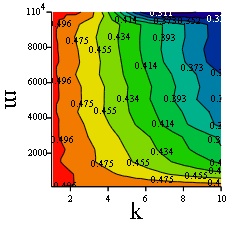
Figure 6.1. Generalization error with respect to $k$ and $m$ for $k^{*}=5$

We now proceed to describe the main result which concerns the relationship between the learner’s performance and the mistake sequence complexity.

6.2. sysRatio $\rho$ versus $k$

First we look at the relationship between the sysRatio $\rho$ and $k$. Figure 6.2 shows the average of the sysRatio $\rho$ as a function of $k$ where in Figure 6.2(A) we used Gzip as the compressor that estimates the Kolmogorov complexity and in Figure 6.2 (B) we used the PPM algorithm as compressor. Note that the PPM compressor obtains $\rho$ values that are smaller than the Gzip compressor which means that the compressed lengths of the corresponding system files is smaller when using PPM. We believe that this is due to additional cost incurred by Gzip in the form of data structures that are appended to the compressed data. This is more noticeable when the file to be compressed is small (for instance, in the plot we see that the the sysRatio only goes below unity at around $k=4$ which is when the uncompressed file length goes above $16$). The PPM compressor thus approximates the algorithmic (Kolmogorov) complexity better than Gzip when the uncompressed files are relatively small. In the remainder of the paper we decided to keep the plots with respect to both types of compressors in order to show that the results of our analysis do not significantly vary as one changes from one type of compressor to another (in some places we put only the Gzip-based results since the differences were insignificant).

Looking at the plots of Figure 6.2 it is clear that the average sysRatio decreases as the learner’s model order $k$ increases. For the PPM compressor, we see a critical point at the vicinity of $k^{*}$ where the convexity of the graph changes from concave down to concave up possibly indicating an inflection point (this holds for learning problems with other values of $k^{*}$, for instance in Appendix A we show this for $k^{*}=3$ and $k^{*}=7$). To explain this, first note that the uncompressed length of the system is always $c\cdot 2^{k}$ for some constant $c>0$ since the vector $d$ is of length $2^{k}$ (see section 5). The length of the compressed system file also grows, but at a slower rate with respect to $k$ and this gives rise to the decrease in $\rho$ with respect to $k$. We can explain why the rate of the compressed system file grows more slowly as follows: for values of $k<k^{*}$ the learner’s model is incapable (by design of the learning problem) of estimating the Bayes optimal prediction and the probability of the events “$b_{i}$ is followed by a $1$” is $p(1|i)=\nicefrac{{1}}{{2}}$ , $1\leq i\leq 2^{k}$. Thus the average value $\hat{p}(1|i)$ of the indicators of such events is a Binomial random variable with a distribution symmetric at $\nicefrac{{1}}{{2}}$ and hence from (5.1) the probability $\alpha_{i}$ that $\hat{p}(1|i)>\nicefrac{{1}}{{2}}$ equals $\nicefrac{{1}}{{2}}$. The components of the random vector $d$ are independent Bernoulli random variables with parameter $\alpha_{i}$ when conditioned on the sample size vector $v$ (this is the vector whose components $v_{i}$ are the number of times that $b_{i}$ appeared in the training sequence, see [19] for details). Since in this case $\alpha_{i}=\nicefrac{{1}}{{2}}$ then each component has a maximum entropy $H(d_{i})=-\alpha_{i}\log\alpha_{i}-(1-\alpha_{i})\log(1-\alpha_{i})=\log 2=1$ and hence the expected value of the entropy of the vector $d$ (with respect to the random sample size vector $v$) is maximal and equals $E_{v}H(d|v)=E_{v}\sum_{i=1}^{2^{k}}H(d_{i}|v_{i})=E_{v}2^{k}=2^{k}.$ Hence the expected compressed length of the system file (which contains the vector $d$) is large as the expected description length of any random variable is at least as large as its entropy.

As $k$ increases beyond $k^{*}$ the model becomes more capable of estimating the true transition probabilities (recall, these are either $0.3$ or $0.7$) and the probability $p(1|i)$ of the events “$b_{i}$ is followed by a $1$” get farther away from $\nicefrac{{1}}{{2}}$ in the direction of $0.3$ or $0.7$, depending on the particular state $i$, $1\leq i\leq 2^{k}$. Thus the average value $\hat{p}(1|i)$ of the indicators of such events is a Binomial random variable with an asymmetric distribution with a mean $p(1|i$). Hence from (5.1) the probability $\alpha_{i}$ that $\hat{p}(1|i)>\nicefrac{{1}}{{2}}$ gets either very close to $0$ or $1$ as the training size $m$ increases. Thus the components of the random vector $d$ tend to be closer to deterministic. They are still random since the training sequence length is not increasing with $k$ and the variance of the estimates $\hat{p}(1|i)$ does not converge to zero. Therefore for each of the $2^{k}$ components of the vector $d$ the entropy is smaller than when $k<k^{*}$. However as there are exponentially many components $d_{i}$, on the whole, the entropy of $d$ (and hence the expected compressed length of the system file) still increases but at a lower rate than when $k<k^{*}$.

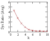
(a) Gzip-based compressor

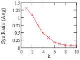
(b) PPM-based compressor

Figure 6.2. The average sysRatio $\rho$ versus model order $k$

We can now alternatively look at the learning curves (section 6.1) based on the sysRatio (instead of $k$). This is shown in Figure 6.3. Clearly, good learners are those with low value of sysRatio $\rho$ (left uppermost region which is colored dark blue) while bad learners are those with a high sysRatio $\rho$, displayed as the rightmost contour which spans from lowest to highest $m$ values.

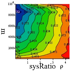
Figure 6.3. Generalization error with respect to $\rho$ and $m$ (for $k^{*}=5$)

We proceed now to discuss the characteristics of the mistake subsequence $\xi_{0}^{(n)}$. First, in section 6.3 we study how its estimated algorithmic complexity $\ell_{0}$ and divergence $\Delta_{0}$ depend on the learner’s decision characteristics, or formally, the sysRatio $\rho$. In section 6.4 we fix the learner’s model order $k$ and study how $\ell_{0}$ depends on $\Delta_{0}$. Finally in sections 6.6 and 6.7 we study the $p_{0}$ and $\rho$ surfaces over the $\Delta\ell$-plane.

6.3. Estimated algorithmic complexity $\ell_{0}$ and divergence $\Delta_{0}$ versus sysRatio $\rho$

Note, in the plots of this section we use the average sysRatio which is computed by taking for each value of $1\leq k\leq 10$ the average over the $N_{k,m}100=1000$ runs. Figure 6.4 shows the graph (with $\mathsf{x}$) of the average estimated algorithmic complexity $\ell_{0}$ of $\xi_{0}^{(n)}$ versus the average system ratio $\rho$. The dashed lines are the upper and lower envelopes of the estimated standard deviation from the mean. This variance arises from the different values of training size $m$ and from the fact that both the training and test sequences are random. The arrow points at the value of $\rho^{*}$ that corresponds to $k^{*}=5$ (the source model order). As can be seen, for low values of $\rho$ the spread in $\ell_{0}$ is low. There is a critical point at $\rho^{*}$ where the spread around the mean value of $\ell_{0}$ increases significantly as $\rho$ increases.

(a) Gzip as compressor

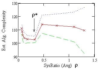
(b) PPM as compressor

Figure 6.4. Estimated algorithmic complexity $\ell_{0}$ of the mistake subsequence $\xi_{0}^{(n)}$ versus the sysRatio (average)

We know from section 3 that the higher the algorithmic complexity of a selection rule the higher the possible deviation of the frequency of $1$s in the selected subsequence (the stochastic deviation). As mentioned above, in [19] it was shown that the decision rule of a learner can be represented as a selection rule that picks the subsequence corresponding to the mistakes made when predicting $0$s in the input test sequence. The theory predicts that the stochastic deviation of the mistake sequence $\xi_{0}^{(n)}$ grows as the complexity of the decision rule increases. We now validate this experimentally.

Figure 6.5 displays the graph (with $\mathsf{x}$) of the average divergence $\Delta_{0}$ of the mistake subsequence $\xi_{0}^{(n)}$ versus the average of the sysRatio $\rho$ where again averages are taken over the $1000$ runs as described above. The dashed lines are the upper and lower envelopes of the standard deviation from the mean. The arrow points at the value of $\rho^{*}$ that corresponds to $k^{*}$ (the source model order). As can be seen, for low values of $\rho$ the spread of $\Delta_{0}$ is low. Similar to the previous result for $\ell_{0}$, also here we see a relative minimum at $\rho^{*}$ where the standard deviation around the mean value of $\Delta_{0}$ increases once we increase $\rho$ beyond $\rho^{*}$. Since we know there is an inverse relationship between $\rho$ and $k$ (Figure 6.2) then the small hook shape that appears to the left of the plot in Figure 6.5 indicates an increase in the $\Delta_{0}$ value as $k$ increases beyond $k^{*}$ ($\rho$ decreases below $\rho^{*}$). Thus data overfitting (which occurs when $k>k^{*)}$ is depicted here via this slight increase in the divergence $\Delta_{0}$ as we decrease $\rho$ beyond the $\rho^{*}$.

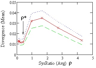
(a) Gzip as compressor

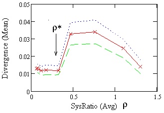
(b) PPM as compressor

Figure 6.5. Divergence $\Delta_{0}$ of the mistake subsequence $\xi_{0}^{(n)}$ versus the sysRatio (averaged)

It follows from this result that the sysRatio $\rho$ (which is a measure of information density of the learner’s model [20]) influences how random are the mistakes made by a learner. The sysRatio $\rho$ is a proper measure of complexity of a learner’s decision rule since it is with respect to $\rho$ that the characteristics of the random mistake subsequence $\xi_{0}^{(n)}$ are consistent with the theory [19, 21], namely, the higher the sysRatio the more significant the deviation $\Delta_{0}$ of $\xi_{0}^{(n)}$ from a pure Bernoulli random sequence.

We have so far considered $\rho$ as an independent variable. In section 6.7 we study the sysRatio as a dependent variable, i.e., as a function of the estimated algorithmic complexity $\ell_{0}$ and divergence $\Delta_{0}$. Before looking at that we proceed to show how $\ell_{0}$ varies with respect to the error $p_{0}$ which will now play the role of the independent variable.

6.4. Estimated algorithmic complexity $\ell_{0}$ versus the error $p_{0}$ for different values of $k$

We first mention that in all the figures below we reduced the number of data points (using simple random sampling) for clarity of presentation. Figure 6.6 shows the estimated algorithmic complexity $\ell_{0}$ of the mistake subsequence $\xi_{0}^{(n)}$ versus the probability of error $p_{0}$. The curves are a second order regression. For $k=3<k^{*}$ there is no clear relationship but for $k=6$ (just above $k^{*})$ we see a sharp rise in $\ell_{0}$ with respect to an increasing $p_{0}$ (the regression polynomial is: $-448x^{2}+396x+47$). When $k=10$ (double the value of $k^{*})$ we see a less steep increase (the regression polynomial is: $-356x^{2}+325x+60$).

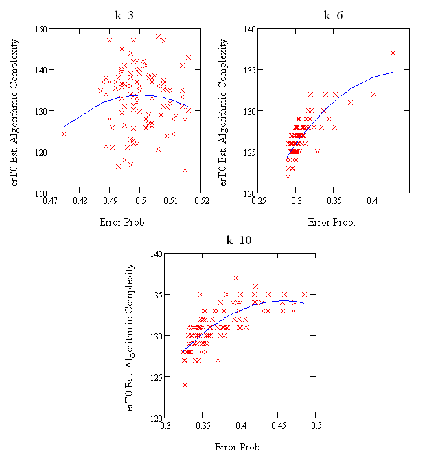
Figure 6.6. Estimated algorithmic complexity $\ell_{0}$ versus error probability, for $k=3$, $6$ and $10$ and $k^{*}=5$ , Gzip-based compressor

6.5. Estimated algorithmic complexity $\ell_{0}$ and divergence $\Delta_{0}$ versus error $p_{0}$ over full range of $m$ and $k$

In Figure 6.7(A) we compare $\ell_{0}$ marked in red ($\mathsf{x}$) to the entropy-based estimate of (4.1) marked in blue ($+$) where we substitute for $n$ in (4.1) the length $n_{0}$ of the sequence $\xi_{0}^{(n)}$ and the probability $p_{0}$ for the parameter $p$. The value of the Pearson’s correlation coefficient between $\ell_{0}$ and the entropy estimate is $0.925$ indicating a high correlation (almost linear). Thus the entropy-based estimate appears to be good for the whole population of learners which consists of training sequences of size $m=100,200,\ldots,10,000$ and models of order $k=1,2,\dots 10$. In Figure 6.7(A) for the $\ell_{0}$ data (marked by $\mathsf{x})$ there appear to be two clusters of points (sequences) separated by an error probability gap at $p_{0}\approx 0.45$. The first region is for $p_{0}<0.38$. We refer to it as the cool cluster. Here the complexity $\ell_{0}$ values are concentrated. The other cluster (termed hot) is where $p_{0}>0.45$. Here the spread in values of $\ell_{0}$ is significantly larger than in the cool cluster.

In Figure 6.7(B) we see that the divergence $\Delta_{0}$ (marked by the symbols $\circ$) and the complexity $\ell_{0}$ (marked by $\mathsf{x}$) are somewhat correlated (Pearson’s coefficient of $0.241$) and it is due to the fact that the divergence values $\Delta_{0}$ are also split into two clusters which are in correspondence with the two clusters of the $\ell_{0}$ values.

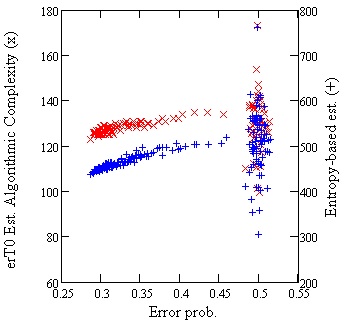
(a) $\ell_{0}$ (marked $\mathsf{x}$) compared to entropy-based estimate (marked $+$) versus $p_{0}$

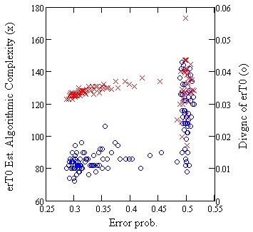
(b) $\ell_{0}$ (marked $\mathsf{x})$ compared to $\Delta_{0}$ (marked $\circ$) versus $p_{0}$

Figure 6.7. Estimated algorithmic complexity $\ell_{0}$ and divergence $\Delta_{0}$ as function of $p_{0}$ , Gzip-based compressor, for population of error sequences based on learners with $m=100,200,\ldots,10,000$ and models of order $k=1,2,\dots 10$.

Let us look at the distribution of $\ell_{0}$ which is shown in Figure 6.8. The distribution is very similar for both types of compressors. For the Gzip-based and PPM-based compressors the mean values are $\mu_{0}=129$, $109$ and the distributions have skewness of $1.79$, $1.8$ and kurtosis of $2.39$, $2.66$, respectively ( for the normal distribution the skewness and kurtosis are $0)$. This indicates that the distributions are positively asymmetric (a heavier right tail) and peaked.

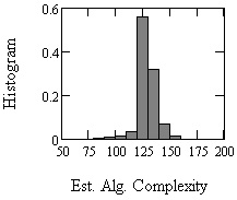
(a) Gzip as compressor

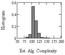
(b) PPM as compressor

Figure 6.8. Histogram of $\ell_{0}$ for population of error sequences based on learners with $m=100,200,\ldots,10,000$ and models of order $k=1,2,\dots 10$.

6.6. The error $p_{0}$ surface

Figure 6.9 depicts the first central result of the paper. It displays the error probability $p_{0}$ as a function of the divergence $\Delta_{0}$ and estimated algorithmic complexity $\ell_{0}$ (we note that the jagged contour lines are due to the interpolation mesh being limited in size and do not reflect actual data). At the center bottom we see the contour level of $0.356$ (this is approximately the Bayes error level) and the topmost contour is at a value of $0.518$ which corresponds to prediction by pure-guessing. We can ascertain the following from this interesting plot: the population of mistake sequences of lowest error probability (close to the Bayes $0.3$ value) concentrates close to the mean value $\mu_{0}$ and has a very low divergence $\Delta_{0}$. This region corresponds to the cool cluster of Figure 6.7 (we call it the cool region and it appears in blue in Figure 6.9). This characteristic indicates that the sequences in the cool region are close to being truly random Bernoulli sequences with parameter $p_{0}$. As we start to look at a population of sequences with a higher error probability $p_{0}$ and walk along its fixed contour level we have a tradeoff between two possible choices: (1) to have a complexity $\ell_{0}$ value which is far from the mean (less than or greater than $\mu_{0}$) and maintain a low divergence $\Delta_{0}$ value or (2) to have a large divergence $\Delta_{0}$ and maintain an $\ell_{0}$ which is close to the mean $\mu_{0}$. The union of the red and orange regions in Figure 6.9 corresponds to the hot cluster that we saw in Figure 6.7. By definition of the maximum a posteriori probability decision rule that we are using the error can never exceed $0.5$ so the true error surface cannot exceed $0.5$ and this is why we see that the empirical error surface ends at a contour level close to $0.5$.

An interesting point that we see here is that this surface is defined only over a part (colored region) of the $\Delta\ell$-plane. We term this the admissible region of the $\Delta\ell$ plane and it is induced by the error surface. In Figure 6.9 we see that the contour area is slightly larger on the right side of $\mu_{0}$ than on the left of $\mu_{0}$ which is consistent with the heavier right tail of the $\ell_{0}$ distribution in Figure 6.8. So admissibility appears to have a slight intrinsic bias towards complexity values $\ell_{0}$ that are larger than the mean $\mu_{0}$.

If we regard sequences in the the cool region as truly random (i.e., having a complexity value $\ell_{0}$ close to the mean $\mu_{0}$ and a low divergence from Bernoulli) then we can introduce a new perspective on the process of learning. When the process is perfect, it produces a Bayes optimal predictor whose mistake sequence falls in the cool region. But when it is imperfect (due to limited training size $m$ or improper model order $k$) the process produces a malformed sequence which is either atypically chaotic ($\ell_{0}$ far from $\mu_{0}$) but stochastic (low $\Delta_{0}$) or typically chaotic ($\ell_{0}$ close $\mu_{0}$) but atypically stochastic (large $\Delta_{0}$).

So far we discussed the error surface which is intrinsically a property of the random mistake sequence since $p_{0}$ is defined only based on the ratio of the number of $1$s to the length of the sequence. In the next section we examine the sysRatio surface which intrinsically is a learner’s characteristic since it measures the information density $\rho$ of the learner’s decision rule.

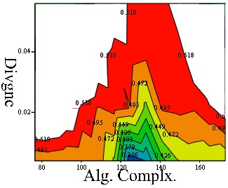
(a) Gzip based compressor

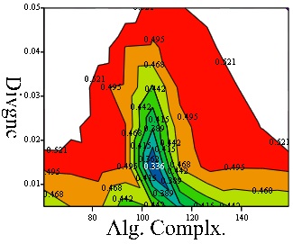
(b) PPM based compressor

Figure 6.9. Error probability $p_{0}$ as a function of divergence $\Delta_{0}$ and estimated algorithmic complexity $\ell_{0}$

6.7. The sysRatio $\rho$ surface

Figure 6.10 displays the next central result of the paper, a contour plot of the sysRatio $\rho$ over the $\Delta\ell$-plane. The outer contours (red) are for higher values of $\rho$. There are two relative minima one of which is at a lower value of $\Delta_{0}$ and touches the $\Delta_{0}=0$ axis while the other appears above the $0.04$ divergence level. Based on what we already know about $\rho$ versus $k$ (Figure 6.2) we can conclude that the lower minimum in Figure 6.10 is in a region of the plane that corresponds to sequences generated by learners of order $k$ which is equal to $k^{*}$ or just slightly above $k^{*}$ (we call this region $OM$ for ’overfitting minimum’) while the upper relative minimum in Figure 6.10 is in the region of sequences generated by learners of order $k$ which is slightly lower than $k^{*}$ (we call this region $UM$ for ’underfitting minimum’). The remaining regions (colored green to red) are where the learners have an order $k$ significantly less than $k^{*}$. Thus there is a saddle point as one passes from $UM$ to $OM$ and cross from $k$ which is just under $k^{*}$ to $k=k^{*}$. This is more pronounced in the Gzip-based compressor than in the PPM-based compressor.

Based on this plot we can see that a decision rule with a high information density (sysRatio value $\rho$) yields an atypically chaotic random error sequence, i.e., with an estimated algorithmic complexity value $\ell_{0}$ that is far from the mean $\mu_{0}$. As the information density of the decision rule decreases the complexity of the error sequence moves towards a typical value ($\ell_{0}$ closer to $\mu_{0}$) and its divergence from Bernoulli decreases towards zero.

(a) Gzip based compressor

(b) PPM based compressor

Figure 6.10. sysratio $\rho$ as a function of divergence $\Delta_{0}$ and estimated algorithmic complexity $\ell_{0}$

Recall from the end of section 2 that the act of predicting bits of the input test sequence $x^{n}$ to be $0$s is equivalent to selecting from $x^{n}$ a subsequence $\xi_{0}^{(n)}$. We are now in a position to understand that this selection process produces random binary sequences $\xi_{0}^{(n)}$ of different character and ’spreads’ them in different regions of the $\Delta\ell$-plane. This spreading is a consequence of what we term scattering bits of a sequence since it resembles particle scattering in physics (it is also similar to the concept of chaotic scattering [17] where instead of initial conditions of the learner we characterize it by its information density $\rho$). Given a random input sequence $x^{(n)}$ the learner (in his decision/selection action) effectively scatters the bits of $x^{(n)}$ in a way that resembles the binary collisions of particles in a beam with other particles that knock the beam particles into different directions. From this scattering the resulting sequence of bits is $\xi_{0}^{(n)}$. The learner here acts as a static structure (a solid of some kind), or a localized target such as a thin foil in a physical scattering experiment. Learners with high information density$\rho$ scatter bits of the input sequence more wildly thereby producing sequences (points in the $\Delta\ell$-plane) that deviate from typical complexity values or have high stochastic divergence. As mentioned in section 1 this is in line with the model introduced in [18] where a static structure is said to deform the randomness characteristics of an input sequence of excitations.

It is interesting to ask at this point whether as a consequence of this phenomenon it may perhaps be possible to optimally fine-tune a learner’s model-order $k$ just by observing the randomness characteristics of the mistake error $\xi_{0}^{(n)}$, i.e., adjusting $k$ in a direction that corresponds to decreasing $\rho$ towards the $OM$ region. It is not yet clear whether such a scheme that monitors the random characteristics of the mistake sequence would yield better performance (either accuracy or computational efficiency) compared to doing standard model-selection which adjusts $k$ directly based on some form of estimate of the generalization error [10].

7. Conclusions

This paper is an experimental investigation of the problem that was posed and theoretically solved in [19, 21]. We have reconfirmed that the sysRatio $\rho$ originally introduced in [24, 22, 23] is a proper measure of the complexity of a learner’s decision rule as it is with respect to $\rho$ that the deformation of randomness of the mistake subsequence $\xi_{0}^{(n)}$ takes place in consistence with the theory, namely, the higher the value of $\rho$ the more significant the divergence $\Delta_{0}$ of the mistake sequence $\xi_{0}^{(n)}$ relative to a pure Bernoulli random sequence. The two central results introduced in the current paper depict the special structure of the error probability $p_{0}$ and sysRatio $\rho$ surfaces over the $\Delta\ell$-plane. They imply that bad learners generate atypically complex or stochastically divergent mistake sequences while good learners generate typically complex sequences with low divergence from Bernoulli. Since a learner can be modeled as a selection rule we name this phenomenon ’bit-scattering’. The idea follows the general model of static algorithmic interference introduced in [18] whereby effectively the learner acts as a static structure whose complexity is the sysRatio (information density $\rho$). It produces randomly-deformed types of mistake sequences where deformation is proportional to $\rho$.

Appendix A  

In this section we present some additional auxiliary results pertaining to the relationship between the sysRatio $\rho$ and model order $k$. In section 6.2 for a learning problem with $k^{*}=5$ we saw that for the PPM-based compressor the graph of the average $\rho$ versus $k$ is decreasing and has a critical point in the vicinity of $k^{*}$. Figure A.1 shows that this critical point also appears in learning problems with $k^{*}=3$. For $k^{*}=7$ there appears to be two critical points, one of which is at $k^{*}$.

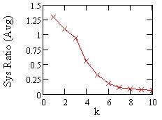
(a) PPM-based compressor, $k^{*}=3$

(b) PPM-based compressor, $k^{*}=7$

Figure A.1. Rates of change of $\rho$ with respect to $k$

References

- [1] M. Anthony and P. L. Bartlett. Neural Network Learning:Theoretical Foundations. Cambridge University Press, 1999.
- [2] A. E. Asarin. Some properties of Kolmogorov random finite sequences. SIAM Theory of Probability and its Applications, 32:507–508, 1987.
- [3] A. E. Asarin. On some properties of finite objects random in an algorithmic sense. Soviet Mathematics Doklady, 36(1):109–112, 1988.
- [4] P. L. Bartlett, S. Boucheron, and G. Lugosi. Model selection and error estimation. Machine Learning, 48:85–113, 2002.
- [5] L. Bienvenu. Kolmogorov-Loveland stochasticity and Kolmogorov complexity. In 24th Annual Symposium on Theoretical Aspects of Computer Science (STACS 2007), volume LNCS 4393, pages 260–271, 2007.
- [6] C. S. Calude. Information and Randomness. Springer, 2002.
- [7] J. Chaskalovic and J. Ratsaby. Interaction of a self vibrating beam with chaotic external forces. Comptes Rendus Mecanique, 338(1):33–39, 2010.
- [8] J.G. Cleary and I.H. Witten. Data compression using adaptive coding and partial string matching. IEEE Transactions on Communications, 32(4):396–402, 1984.
- [9] T. M. Cover and J. A. Thomas. Elements of information theory. Wiley-Interscience, New York, NY, USA, 2006.
- [10] L. Devroye, L. Gyorfi, and G. Lugosi. A Probabilistic Theory of Pattern Recognition. Springer Verlag, 1996.
- [11] B. Durand and N. Vereshchagin. Kolmogorov-Loveland stochasticity for finite strings. Information Processing Letters, 91(6):263–269, 2004.
- [12] M. Hutter. Universal Artificial Intelligence: sequential decisions based on algorithmic probability. Springer, 2004.
- [13] A. N. Kolmogorov. Three approaches to the quantitative definition of information. Problems of Information Transmission, 1:1–17, 1965.
- [14] A. N. Kolmogorov. On tables of random numbers. Theoretical Computer Science, 207(2):387–395, 1998.
- [15] D. W. Loveland. A new interpretation of the von Mises’ concept of random sequence. Zeitschrift fur mathematische Logik und Grundlagen der Mathematik, 12:279–294, 1966.
- [16] P. Martin-Löf. The definition of random sequences. Information and Control, 9:602–619, 1966.
- [17] E. Ott and T. Tel. Chaotic scattering: an introduction. Chaos, 3(4), 1993.
- [18] J. Ratsaby. An algorithmic complexity interpretation of Lin’s third law of information theory. Entropy, 10(1):6–14, 2008.
- [19] J. Ratsaby. How random are a learner’s mistakes ? Technical Report # arXiv:0903.3667, 2009.
- [20] J. Ratsaby. Learning, complexity and information density. Technical Report # arXiv:0908.4494v1, 2009.
- [21] J. Ratsaby. Randomness in learning. In Proc. of IEEE International Conference on Computational Cybernetics, (ICCC’09), pages 141–145, 2009.
- [22] J. Ratsaby. Some consequences of the complexity of intelligent prediction. Presented at International symposium on understanding intelligent and complex systems (UICS’09), Petru Maior University, 2009.
- [23] J. Ratsaby. Some consequences of the complexity of intelligent prediction. Broad Research in Artificial Intelligence and Neuroscience, 1(3):113–118, 2010.
- [24] J. Ratsaby. Learning, complexity and information density. Acta Universitatis Apulensis, accepted.
- [25] J. Ratsaby and I. Chaskalovic. Random patterns and complexity in static structures. In Proc. of International Conference on Artificial Intelligence and Pattern Recognition (AIPR’09), volume III of Mathematics and Computer Science, pages 255–261, 2009.
- [26] J. Ratsaby and I. Chaskalovic. On the algorithmic complexity of static structures. Journal of Systems Science and Complexity, 23(6), 2010. doi:10.1007/s11424-010-8465-2.
- [27] J. Ratsaby, R. Meir, and V. Maiorov. Towards robust model selection using estimation and approximation error bounds. In Proc. of Ninth Ann. Conf. on Comp. Learn. Theor., pages 57–67. ACM, 1996.
- [28] V.A. Uspenskil, A. L. Semenov, and A. Kh. Shen. Can and individual sequence of zeros and ones be random ? Russian Mathematical Surveys, 45(1):121–189, 1990.
- [29] V. V. Vyugin. Algorithmic complexity and stochastic properties of finite binary sequences. The Computer Journal, 42:294–317, 1999.
- [30] J. Ziv and A. Lempel. A universal algorithm for sequential data compression. IEEE Transactions on Information Theory, 23(3):337–343, 1977.