Could Leptons, Quarks or both be Highly Relativistic Bound States of Minimally Interacting Fermion and Scalar?

Abstract

The possibility that leptons, quarks or both might be highly relativistic bound states of a spin-0 and spin-1/2 constituent bound by minimal electrodynamics is discussed. Typically, strongly bound solutions of the Bethe-Salpeter equation exist only when the coupling constant is on the order of or greater than unity. For the bound-state system discussed here, there exist two classes of boundary conditions that could yield strongly bound solutions with coupling constants on the order of the electromagnetic fine structure constant $\alpha$. In both classes the bound state must have spin one half, thus providing a possible explanation for the absence of higher-spin leptons and quarks.

I Motivation for Composite Models of Leptons and Quarks

The motivation for studying composite models of leptons and quarks is almost entirely circumstantial. Three times in the past 150 years particles that were - or are currently - thought to be elementary could be organized into families: (1) In the 1860’s Meyer and Mendelev arranged the atoms into the periodic table that consists of 18 families. The existence of families was ultimately explained by the realization that atoms are composite. (2) Almost 100 years later two of the then-fundamental particles, the neutron and proton - as well as many other baryons and mesons - were placed into SU(3) multiplets with the ultimate result that the neutron and proton were no longer viewed as being fundamental but instead were comprised of quarks Gell-Mann (1964); Zweig (1964). (3) By the mid 1970’s many physicists realized that the charged leptons, the neutrinos, the positively charged quarks and the negatively charged quarks constitute four families. Today the three charged families are known to have three members each, and the neutrino family almost certainly has three members as well Amsler  et al. (2008). Because the existence of families of “fundamental” particles has twice been explained by the realization that the particles are actually composite, although speculative, as is any physics beyond the standard model, the most conservative approach to explain the existence of the lepton and quark families likely is to assume that the particles are composite. In the 1970’s the hypothetical constituents of quarks and leptons were given the name “preons” Pati and Salam (1974).

The circumstantial evidence for composite leptons and quarks is certainly not conclusively corroborated by direct experimental evidence. The factor $g_{\mu}$ relates the muon’s magnetic moment ${\boldsymbol{\mu}}$ and spin ${\boldsymbol{s}}$ according to the relation,

$${\boldsymbol{\mu}}=g_{\mu}\frac{e\hbar}{2m_{\mu}c}{\boldsymbol{s}}\,,\hskip 28.45274ptg_{\mu}=2(1+a_{\mu})\,.$$ (1)

The present experimental world average determination for $a_{\mu}$ Bennett  et al. (2004) is $a_{\mu}^{\mathrm{exp}}=116592080(63)\times 10^{-11}\,.$ The primary source of error in the theoretical calculation of $a_{\mu}$ arises from the contribution of the strong force, which cannot be calculated from first principles but, instead, must be determined from experimental data. A direct determination of the contribution from strong interactions uses experimental data from electron-positron collisions, and the theoretical value calculated from the standard model is de Rafael (2009) $a_{\mu}^{\mbox{SM direct}}=(116591785\pm 51)\times 10^{-11}$. The theoretical value in is smaller than the experimental value by 3.6 $\sigma$. The indirect method Davier  et al. (2009) uses experimental data from hadronic tau decays, conservation of the vector current and isospin corrections and yields the value $a_{\mu}^{\mbox{SM indirect}}=(116591932\pm 52)\times 10^{-11}$, which is 1.8 $\sigma$ below the experimental value. The discrepancy suggests that there is physics beyond the standard model. But in addition to muon substructure, the discrepancy could also be explained, for example, by the existence of supersymmetric particles or by composite $W$ and $Z$ bosons.

If leptons, quarks or both are composite, several characteristics that any composite model must possess can immediately be determined from the mass- and spin-spectra of the leptons and quarks. The masses of the charged leptons and quarks satisfy the inequalities ${\rm m}_{\rm electron}\ll{\rm m}_{\rm muon}\ll{\rm m}_{\tau}$, ${\rm m}_{\rm up}\ll{\rm m}_{\rm charm}\ll{\rm m}_{\rm top}$, and ${\rm m}_{\rm down}\ll{\rm m}_{\rm strange}\ll{\rm m}_{\rm bottom}$. Since no structure has been conclusively detected for leptons or quarks, any composite system must be very strongly bound. This precludes a composite model whereby, for example, the electron, muon, and tau are successively much more massive because one or more of their constituents are successively much more massive. The large differences in the masses of the particles in each family are consistent with strong binding only if the bound system is highly relativistic.

Even though the existence of families is explained by the atomic model of atoms, the quark model for mesons and baryons and, as discussed here, perhaps a preon model for leptons and quarks, each of the composite models is radically different. In the atomic model, aside from small mass defects, the mass of an atom is the sum of the masses of the constituents. For mesons and baryons, most of the mass results from the kinetic energy of the quarks so the mass of a meson or baryon is substantially greater than the sum of the masses of the constituent quarks. If leptons, quarks or both are highly relativistic bound states, the mass of each lepton or quark is less - and for the least massive particle in each family, much less - than the sum of the masses of the constituents.

For simplicity the bound system would likely be comprised of two or three constituents. If the composite system were comprised of a spin-0 boson and a spin-1/2 fermion, then, in the language of non-relativistic physics, if all states have zero orbital angular momentum, all would have total angular momentum or spin one half. For the relativistic equation discussed here, a similar mechanism allows strongly bound states only when the total angular momentum or spin is one half. If the composite system were comprised of three or more constituents, it is difficult to find a mechanism that would prevent higher-spin bound states.

Many physicists in the 1970’s studied the possibility that quarks and leptons might be bound states of preons Marshak (1993). Assuming the existence of only a few preons, the existence of all quarks and leptons could be explained with each being a preon bound state. In the book The Trouble with Physics Smolin (2006), Smolin writes, “Unfortunately, there were major questions that the preon theories were not able to answer. These have to do with the unknown force that must bind the preons together into the particles that we observe. The challenge was to keep the observed particles as small as they are while keeping them very light. Because preon theorists couldn’t solve this problem, preon models were dead by 1980.”

Leptons interact gravitationally, weakly, and electromagnetically. Among the three forces, the electromagnetic interaction is the only one that might be able to provide the requisite strong binding. At sufficiently high energies, the electromagnetic interaction must, of course, be replaced by the electroweak interaction, but this added complication is not incorporated in the Bethe-Salpeter equation discussed here. The similarities of the charged lepton and quark mass spectra suggest that the same mechanism might be responsible for binding in all four families. Such a scenario could occur if only one of the two quark constituents interacted strongly so that the pair would not. A heretofore unknown interaction might, of course, be responsible for the binding, but assuming the existence of such a force would represent a much more speculative approach.

A few nonrelativistic and partially relativistic calculations suggest that electromagnetism might be able to create a bound state with the properties of quarks and leptons. Using the Schrödinger equation in two space dimensions, a charged quanta interacting with a charged magnetic dipole was shown to create bound states such that all low-energy states have zero orbital angular momentum Mainland and Scott (1983). The Dirac equation was used to show that strongly bound states can occur when a spin-1/2 quanta interacts with a charged magnetic dipole Barut and Kraus (1976), and the Klein-Gordon equation in two space dimensions was used to show that a charged quanta interacting with a charged magnetic dipole can create bound states such that the energy gap increases between successively higher bound states Mainland and Scott (1984).

But, as previously mentioned, by about 1980 most physicists had given up on the idea: experimentally there was no conclusive evidence that quarks or leptons were composite, a situation that has not changed significantly in the intervening thirty years, and theoretically no one could find a way to create bound states that both possessed the correct mass spectra and also were extremely small. The Bethe-Salpeter equation Salpeter and Bethe (1951) provided a theoretical framework for studying relativistic bound states. Also, by the late 1960’s two, two-body, bound-state Bethe-Salpeter equations with unphysical interactions had been completely solved. However, in 1980 a general, numerical technique for solving the two-body, bound-state Bethe-Salpeter equation had not been developed, and the high-speed computers required to solve the bound-state equation when the preons interact via minimal electrodynamics did not exist. With the development of super computers and a general method for solving the two-body, bound-state Bethe-Salpeter equation Mainland (2005), the properties of relativistic bound states can now be determined, providing motivation to revisit preon models.

II Possible Preon Model of Leptons and Quarks

If the charged lepton family, the neutrino family, the negatively charged quark family, and the positively charged quark family are each a bound state of a different combination of a spin-0 and a spin-1/2 preon that interact via minimal electrodynamics, then all four families could be created from just two fermion preons and two boson preons. Each of the two boson preons can bind with each of the two fermion preons to create four different bound states or four families as indicated in Table 1. Also, as indicated in Table 1, the sum of the charges of the two constituent preons must equal the charge of the leptons or quarks in the family that the preons combine to create, yielding four equations for the charges of the four preons.

Table 1: Preon charges and constraints that the preon charges must obey

Family	Preon	Preon	Constraint
	Fermion	Boson
	Charge	Charge
Electron	$\hskip 8.5359ptq_{f1}$	$\hskip 11.38092ptQ_{S1}$	$q_{f1}+Q_{S1}=-1$
Neutrino	$\hskip 8.5359ptq_{f2}$	$\hskip 11.38092ptQ_{S1}$	$q_{f2}+Q_{S1}=0$
Negative Quarks	$\hskip 8.5359ptq_{f1}$	$\hskip 11.38092ptQ_{S2}$	$q_{f1}+Q_{S2}=-\frac{1}{3}$
Positive Quarks	$\hskip 8.5359ptq_{f2}$	$\hskip 11.38092ptQ_{S2}$	$q_{f2}+Q_{S2}=\frac{2}{3}$

Only three of the equations are independent. Possible preon charges $\leq 2$ that are multiples of $\pm\frac{1}{3}$ are as follows:

Table 2: Possible charges of preon fermions and bosons

Preon Fermion Charges		Preon Boson Charges
$q_{f1}$	$q_{f2}$	$Q_{S1}$	$Q_{S2}$
1	2	-2	$-\frac{4}{3}$
$\frac{2}{3}$	$\frac{5}{3}$	$-\frac{5}{3}$	$-1$
$\frac{1}{3}$	$\frac{4}{3}$	$-\frac{4}{3}$	$-\frac{2}{3}$
$-\frac{4}{3}$	$-\frac{1}{3}$	$\frac{1}{3}$	$1$
$-\frac{5}{3}$	$-\frac{2}{3}$	$\frac{2}{3}$	$\frac{4}{3}$
$-2$	$-1$	$1$	$\frac{5}{3}$

III Introduction to the Bethe-Salpeter Equation

For relativistic, two-body, bound-state systems, a few analytical, Bethe-Salpeter solutions exist, but only in the limit that the binding energy equals the sum of the masses of the two constituent particles, implying the the energy of the bound state is zero. These solutions are not physical because they are calculated in the center-of-mass rest frame. But if a bound state has zero rest energy, it must travel at the speed of light. Therefore, zero-energy solutions are the zero-energy limit of physical solutions. In this limit the equation is always invariant under rotations in Minkowski space and so is separable.

Analytical solutions have been obtained in the zero-energy limit, for example, for the Wick-Cutkosky Model Wick (1954); Cutkosky (1954) that consists of two scalars with arbitrary, nonzero masses bound by the exchange of a massless scalar. A variety of exact solutions have been obtained for two spinors with equal masses that are bound by the exchange of a massless scalar Goldstein (1953); Kummer (1964); Suttorp (1975) or a massless vector Nishimura and Higashijima (1975). An exact solution has also been found for two spinors with unequal, nonzero masses bound by the exchange of a massless scalar Keam (1971).

Even when the energy is zero, most solutions are numerical. For example, such solutions have been obtained for two scalars with unequal, nonzero masses bound by the exchange of a massive scalar Brennan (1975) and for a scalar and a spinor with arbitrary, nonzero masses bound by the exchange of a massless scalar Mainland (2003a, b) or a massless vector Mainland (2008). When the energy is nonzero, all solutions are numerical.

Only four, two-body, bound-state Bethe-Salpeter equations have been completely solved. That is, solved for arbitrary values of energy and arbitrary values of the masses of the two constituents. (1) The Wick-Cutkosky Model consists of two scalars with arbitrary, nonzero masses bound by the exchange of a massless scalar Wick (1954); Cutkosky (1954); zur Linden and Mitter (1969). (2) The Scalar-Scalar Model consists of two scalars with arbitrary, nonzero masses bound by the exchange of a massive scalar Schwartz (1965); Kaufmann (1969); zur Linden (1969a, b). (3) The Scalar Electrodynamics Model consists of a scalar and a fermion with arbitrary, nonzero masses bound by the exchange of a massless scalar Mainland (2005). (4) The Fermion-Scalar Model consists of a scalar and a fermion with arbitrary, nonzero masses bound by the exchange of a massive scalar Mainland (2006).

The interaction of the preons and the electromagnetic field is described by the renormalizable interaction Lagrangian,

$$L_{\rm int}= :-q_{f}A^{\mu}\bar{\psi}\gamma_{\mu}\psi+\imath Q_{s}\,A_{\mu}\,[\phi\,(\partial^{\mu}\phi^{\dagger})-(\partial^{\mu}\phi)\,\phi^{\dagger}]$$

$$+Q_{s}^{2}A^{\mu}A_{\mu}\phi\,\phi^{\dagger}:\,.$$ (2)

The proposed preon model of leptons, quarks or both is a bound state of a spin-1/2 fermion with charge $q_{f}$ and mass m_f represented by the field $\psi$ and a scalar with charge $Q_{s}$ and mass m_s represented by the field $\phi$. The fermion and scalar fields interact minimally with the electromagnetic field $A_{\mu}$.

The Bethe-Salpeter equation will be used to study the properties of the bound state. Since every Feynman diagram contributes to the exact equation, some approximation must be made. Usually only the effect of the lowest-order diagram shown below is included. Because of the structure of the Bethe-Salpeter equation, contributions from the diagram and iterations of the diagram, which form a ladder with the photon propagator forming the rungs, contribute. Thus the approximation is called the ladder approximation.

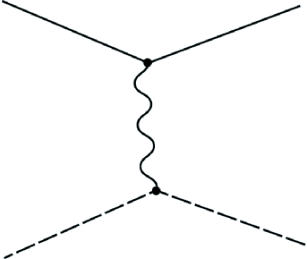
$\phi$                                               $\phi$

$Q_{s}$

$A^{\mu}$

$q_{f}$

$\psi$

$\psi$

Figure 1: Lowest-order Feynman diagram for a spin-1/2 field $\psi$ with charge $q_{f}$ and a scalar field $\phi$ with a charge $Q_{s}$ interacting via minimal electrodynamics with the photon field $A^{\mu}$.

In the ladder approximation the two-body, bound-state Bethe-Salpeter equation describing a spin-0 boson and a spin-1/2 fermion bound by minimal electrodynamics is

$$[(p^{0} +\xi E)\gamma_{0}+p^{i}\gamma_{i}-m_{f}]$$

$$\times\{[p^{0}+(\xi-1)E]^{2}-{\boldsymbol{p}}^{2}-m_{s}^{2}\}\chi(p)$$

$$=\frac{iq_{f}Q_{s}}{(2\pi)^{4}}\int_{-\infty}^{\infty}\frac{{\rm d}^{4}q}{(p-q)^{2}+i\varepsilon}\{\gamma^{0}[p_{0}+q_{0}+2(\xi-1)E]$$

$$+\gamma^{i}(p_{i}+q_{i})\}\chi(q)\,.$$ (3)

The equation has been written in the center-of-mass rest frame where the four-momentum $K^{\mu}$ of the bound state takes the form $K^{\mu}=(E,0,0,0)$. In the non-relativistic limit $\xi=m_{f}/(m_{f}+m_{s})$.

If the binding were non-relativistic, the properties of the bound states could be calculated using the Schrödinger equation,

$$H(x)\psi(x)=E\psi(x)\,.$$ (4)

There are a number of notable differences between the bound-state Schrödinger and Bethe-Salpeter equations: a) Because the energy $E$ appears multiple times in the Bethe-Salpeter equation (III), a Hamiltonian does not exist for the relativistic problem. b) Because $E$ appears multiple times in the Bethe-Salpeter equation, the equation is solved by specifying the energy and solving for the coupling constant $q_{f}Q_{s}/(4\pi)$ as an eigenvalue. The process for solving the Schrödinger equation (4) is the reverse: the coupling constant is specified, and the energy $E$ is solved for as an eigenvalue. The two procedures yield equivalent information. (c) There is no action at a distance for the Bethe-Salpeter equation since the interaction is covariant. (d) The Bethe-Salpeter is an integral equation; therefore, boundary conditions are incorporated in the equation. (e) The Bethe-Salpeter equation is separable when energy $E=0$ and is almost always nonseparable when $E\neq 0$.

The author has developed a systematic method Mainland (2005) for solving the two-body, bound-state Bethe-Salpeter equation for arbitrary values of energy. However, to show how specific boundary conditions allow for the possibility that strongly bound solutions exist when the coupling constant $q_{f}Q_{s}/(4\pi)$ is on the order of the fine structure constant $\alpha$, here attention is restricted to the strong binding limit $E=0$.

IV Strongly Bound Solutions

To solve the Bethe-Salpeter equation in the strong-binding (zero-energy) limit, the singularity in the kernel of the Bethe-Salpeter equation is removed, and the equation is transformed from Minkowski to Euclidean space by making a Wick rotation Wick (1954), which is always possible in the ladder approximation.

In the zero-energy limit the angular dependence of the equation separates Sugano and Munakata (1956) when solutions are written as products of the functions $\Psi^{(+)}_{1}$ and $\Psi^{(+)}_{2}$ that are four-component hyperspherical harmonics in four-dimensional, Euclidean space-time and the functions $F(|p|)$ and $G(|p|)$ that depend only on the magnitude of the Euclidean four-momentum $|p|$,

$$\chi(ip^{0},{\bf p}) =F(|p|)\Psi^{(+)}_{1}(\cos\,\theta_{1},\theta_{2},\phi)$$ (5)

$$+G(|p|)\Psi^{(+)}_{2}(\cos\,\theta_{1},\theta_{2},\phi)\,.$$

The four-component hyperspherical harmonics $\Psi^{(+)}_{1}$ and $\Psi^{(+)}_{2}$ in (5) are analogous to the two-component spherical harmonics $\phi^{(\pm)}_{j,m}$ Bjorken and Drell (1965) that are used to separate the Dirac equation with a spherically symmetric potential. Using hyperspherical harmonics in four-dimensional space as part of the basis functions both decreases the number of integrations that must be performed numerically and prevents the appearance of a logarithmic singularity in the kernel. The separated, zero-energy Bethe-Salpeter equation is

$$\left[|p|^{2}+(1+\Delta)^{2}\right]\left[(1-\Delta)F^{(+)}(|p|)+|p|G^{(+)}(|p|)\right]$$

$$=-\frac{q_{f}Q_{s}}{(2\pi)^{4}}|p|\int_{0}^{\infty}|q|^{3}\Lambda^{(2)}_{k_{1}+1/2}(|p|,|q|)G^{(+)}(|q|)\mathrm{d}|q|$$

$$-\frac{q_{f}Q_{s}}{(2\pi)^{4}}\int_{0}^{\infty}|q|^{4}\Lambda^{(2)}_{k_{1}-1/2}(|p|,|q|)G^{(+)}(|q|)\mathrm{d}|q|\,,$$ (6a)

$$\left[|p|^{2}+(1+\Delta)^{2}\right]\left[-|p|F^{(+)}(|p|)+(1-\Delta)G^{(+)}(|p|)\right]$$

$$=\frac{q_{f}Q_{s}}{(2\pi)^{4}}|p|\int_{0}^{\infty}|q|^{3}\Lambda^{(2)}_{k_{1}-1/2}(|p|,|q|)F^{(+)}(|q|)\mathrm{d}|q|$$

$$+\frac{q_{f}Q_{s}}{(2\pi)^{4}}\int_{0}^{\infty}|q|^{4}\Lambda^{(2)}_{k_{1}+1/2}(|p|,|q|)F^{(+)}(|q|)\mathrm{d}|q|\,.$$ (6b)

In the above equation the index $k_{1}=1/2,3/2,\dots$ and

$$\Lambda^{(2)}_{n}(|p|,|q|)=\left\{\begin{array}[]{lcc}\frac{2\pi^{2}}{|p||q|}\;\frac{(\frac{|q|}{|p|})^{n+1}}{n+1}&\mathrm{if}&|q|\leq|p|\,,\\ \\ \ \frac{2\pi^{2}}{|p||q|}\;\frac{(\frac{|p|}{|q|})^{n+1}}{n+1}&\mathrm{if}&|q|\geq|p|\,.\\ \end{array}\right.$$ (10)

Dimensionless variables have been introduced in (6) by defining $m_{f}\equiv m(1-\Delta),m_{s}\equiv m(1+\Delta),p^{\prime}\equiv p/m$ and $q^{\prime}\equiv q/m$. Then primes have been omitted for all momentum variables since all are dimensionless.

Eq. (6) is solved by expanding the functions $F(|p|)$ and $G(|p|)$ in terms of a finite set of basis functions that (very nearly) obey the boundary conditions that $F(|p|)$ and $G(|p|)$, respectively, obey.

$$\mbox{basis function}=\mbox{convergence function}\times\mbox{spline}$$ (11)

The convergence function depends on the magnitude of the four-momentum $|p|$ and obeys the boundary conditions that the solution obeys. A general method for analytically calculating boundary conditions for Bethe-Salpeter equations has been developed Mainland (2003b). Typically, as is the case for the Bethe-Salpeter equation being discussed here, the behavior of the solution at small momenta $|p|$ can be determined exactly; however, at large $|p|$ boundary conditions can sometimes only be determined within ranges, complicating the calculation. If the solution $F(|p|)$ obeys the boundary conditions

$$F(|p|)_{\stackrel{{\scriptstyle\displaystyle\longrightarrow}}{{|p|\rightarrow 0}}}|p|^{f_{0}}\,,\hskip 28.45274ptF(|p|)_{\stackrel{{\scriptstyle\displaystyle\longrightarrow}}{{|p|\rightarrow\infty}}}|p|^{-f_{\infty}}\,,\\$$ (12)

then the convergence function for $F(|p|)$ is given by

$$\mbox{convergence function}=\frac{|p|^{f_{0}}}{(|p|+{\rm constant})^{f_{0}+f_{\infty}}}\,.\\$$ (13)

Cubic splines $B_{i}(|p|)$ de Boor (1978) are defined on four contiguous intervals, and the value of $|p|$ at the boundary of each interval is called a “knot” that is denoted by $T_{j}$. Within each interval a cubic spline is a cubic polynomial with coefficients chosen so that the cubic spline and its first two derivatives are continuous, implying that a cubic spline and its first two derivatives vanish at the beginning of the first interval and at the end of the fourth. The single, remaining, unspecified coefficient is fixed by an overall normalization condition. The spline $B_{i}(|p|)$ begins at the knot $T_{i}$ and terminates at $T_{i+4}$. A major advantage of using splines, instead of functions defined on the entire interval $0\leq|p|\leq\infty$, is that, by concentrating knots in the region where the solution is changing most rapidly, more splines are available where they are most needed to represent a solution. Additionally, it is much faster to integrate numerically over splines because they are nonzero only on a finite interval.

#1      #2            #3          #4

$B_{i}(|p|)$

$T_{i}$  $T_{i+1}$       $T_{i+2}$             $T_{i+3}$ $T_{i+4}$

        $|p|$

Figure 2: Cubic spline $B_{i}(|p|)$ plotted as a function of the magnitude of the four-momentum $|p|$.

Because the convergence function obeys the boundary conditions exactly at large and small $|p|$, and because the splines also depend on $|p|$, the basis functions very nearly obey the boundary conditions, but they do not obey the boundary conditions exactly. However, linear combinations of these basis functions obey the boundary conditions exactly and almost always yield convergent series expansions for solutions.

The zero-energy equation is discretized and then solved by converting it into a generalized matrix eigenvalue equation using the Rayleigh-Ritz-Galerkin variational method Delves and Walsh (1974); Atkinson (1976).

Typically strongly bound solutions of the Bethe-Salpeter equation exist only when the coupling constant $q_{f}Q_{s}/(4\pi)$ is on the order of or greater than unity. If solutions exist for $q_{f}Q_{s}/(4\pi)\sim\alpha$, then at least one integral in (6) must be very large. Two sets of boundary conditions Mainland (2008) could yield one or more large integrals, and in both cases the integrals could be large when the coupling constant is small only if the spin of the bound state is one half. If leptons, quarks or both are composite, this mechanism would explain why leptons, quarks or both all have spin one half. Here attention is restricted to the following boundary conditions:

$$F(|p|)\xrightarrow[|p|\rightarrow\infty]{}F_{\infty}\;|p|^{-(k_{1}+\frac{7}{2})}\,,$$ (14a)

$$G(|p|)\xrightarrow[|p|\rightarrow\infty]{}G_{\infty}\;|p|^{-(k_{1}+\frac{5}{2}+\epsilon_{g})}\,.$$ (14b)

In (11), $k_{1}=j,j+1,\dots$, and $F_{\infty}$ and $G_{\infty}$ are constants. The parameter $\epsilon_{g}$ satisfies the conditions $0<\epsilon_{g}<2$ if $k_{1}=1/2$, and $0\leq\epsilon_{g}<2$ if $k_{1}\geq 3/2$.

For solutions satisfying the boundary conditions (11), in the limit of large $|p|$, the Bethe-Salpeter equation (IV) decouples from (IV) and takes the form

$$G_{\infty}|p|^{-k_{1}+1/2-\epsilon_{g}}\xrightarrow[|p|\rightarrow\infty]{}-\frac{q_{f}Q_{s}}{4\pi}\frac{1}{2\pi}\times$$

$$\left[\frac{2(k_{1}+1)}{(k_{1}+\frac{1}{2})(k_{1}+\frac{3}{2})}|p|^{-(k_{1}+3/2)}\int_{0}^{|p|}{\rm d}|q||q|^{k_{1}+7/2}G(|q|)\right.$$

$$+\frac{|p|^{k_{1}+3/2}}{k_{1}+\frac{3}{2}}G_{\infty}\int_{|p|}^{\infty}{\rm d}|q||q|^{-(2k_{1}+2+\epsilon_{g})}$$

$$\left.+\frac{|p|^{k_{1}-1/2}}{k_{1}+\frac{1}{2}}G_{\infty}\int_{|p|}^{\infty}{\rm d}|q||q|^{-(2k_{1}+\epsilon_{g})}\right]\,.$$ (15)

Only the final integral in (IV) can be large and then iff $k_{1}=1/2$ and $\epsilon_{g}\ll 1$. Since $k_{1}=j,j+1,\dots$, and $k_{1}=1/2$ for all strongly bound states with small coupling constants, all such states have total angular momentum or spin one half.

Using expressions for the integrals in (IV) that are valid in the limit of large $|p|$ Mainland (2003b), the following expression is obtained for the coupling constant when $k_{1}=1/2$:

$$\frac{q_{f}Q_{s}}{4\pi}=-\frac{\pi}{2}\frac{\epsilon_{g}(2-\epsilon_{g})(2+\epsilon_{g})}{(1+\epsilon_{g})}\,.$$ (16)

For small values of $\epsilon_{g}$, the coupling constant $q_{f}Q_{s}/(4\pi)$ is small.

It is particularly difficult to obtain solutions when a fermion and scalar interact via minimal electrodynamics instead of through the exchange of a massless or massive scalar. As can be seen from the dependence of the coupling constant on $\epsilon_{g}$, the solutions go to zero at large momenta sufficiently slowly that the behavior of solutions at large momenta has a very significant effect on the coupling constants.

V Summary

Three major points are made in the talk: a) It might be possible to describe leptons, quarks or both as highly relativistic bound states of a spin-0 and spin-1/2 constituent bound by minimal electrodynamics. b) Strongly bound states with coupling constants on the order of the electromagnetic fine structure constant $\alpha$ are allowed by the boundary conditions and likely exist. c) All such strongly bound states would have spin one half, as do the leptons and quarks.