HD 172189: another step in furnishing one of the best laboratories known for asteroseismic studies

HD 172189 is a spectroscopic eclipsing binary system with a rapidly-rotating pulsating $\delta$ Scuti component. It is also a member of the open cluster IC 4756. These combined characteristics make it an excellent laboratory for asteroseismic studies. To date, HD 172189 has been analysed in detail photometrically but not spectroscopically. For this reason we have compiled a set of spectroscopic data to determine the absolute and atmospheric parameters of the components. We determined the radial velocities (RV) of both components using four different techniques. We disentangled the binary spectra using KOREL, and performed the first abundance analysis on both disentangled spectra. By combining the spectroscopic results and the photometric data, we obtained the component masses, 1.8 and 1.7 M_⊙, and radii, 4.0 and 2.4 R_⊙, for inclination $i=73.2^{\circ}$, eccentricity $e=0.28$, and orbital period $\Pi=5.70198$ days. Effective temperatures of 7600 K and 8100 K were also determined. The measured $v\sin i$ are 78 and 74 km s^-1, respectively, giving rotational periods of 2.50 and 1.55 days for the components. The abundance analysis shows [Fe/H] = –0.28 for the primary (pulsating) star, consistent with observations of IC 4756. We also present an assessment of the different analysis techniques used to obtain the RVs and the global parameters.

1 Introduction

HD 172189 (=BD +5 3864, $V=8.85$ mag, $\alpha=18^{\rm h}$38^m37.6^s, $\delta=+05^{\rm d}27^{\rm m}55.3^{\rm s}$, J2000) has the combined characteristics of being an eclipsing and spectroscopic binary, pulsating star, and member of a cluster (Martin 2003, Martín-Ruiz et al. 2005 — MR05 hereafter, Costa et al. 2007, Ibanoǧlu et al. 2009 — I09 hereafter). Each of these provide unique constraints that allow us to test stellar evolution theories in an independent form: a) an eclipsing spectroscopic binary system is fundamental for determining the absolute global parameters of both stars and the system with precision; b) a pulsating star allows us to use the oscillation frequencies to probe the interior of the star, thereby also determining the evolutionary state; c) cluster membership has the distinct advantage that the properties such as age, metallicity, and distance can be well-determined. Given the constraints imposed by the cluster membership and the binary system on the mass, age, and metallicity of the pulsating star, the observed seismic frequencies can be used to test and improve the current asteroseismic models. For example, as both components are rapidly rotating with periods of 2.50 and 1.55 days, (see Sect.5), we can investigate the effects of rotation, such as the mixing of elements and transport of angular momentum. Several theories exist regarding rapid rotation, but as yet, observations have not been able to confirm any of these hypotheses. Some examples of these unproved theories include understanding the interplay between rapid rotation and convective cores, enabling the transport of angular momentum both poleward and in the radial direction (Featherstone et al. 2007), or the existence of an overshoot boundary layer between the convective core and the radiative region, where mixing of nuclear elements can influence main sequence lifetimes (Brun et al. 2004). Such theories can be confirmed from detailed seismic modeling, once the global parameters of the pulsating star have been determined.

Since HD 172189 was discovered to be a binary system by Martin (2003), several groups have shown a keen interest in this object. Dedicated photometric campaigns (Amado et al. 2006, MR05, Costa et al. 2007, I09) have begun to reveal the true nature of this system, and several oscillation frequencies have been documented from the time series of the $\delta$ Scuti star. This system is moreover a selected target of the asteroseismic core program of the CoRoT satellite mission (Baglin et al. 2006a,b, Michel et al. 2008), and has been continuously observed from space in white light for about 150 days from April to September 2008, with the aim of interpreting the pulsations.

With the prospects of using the observed oscillation frequencies to study the internal structure of the star, we have compiled spectroscopic data taken in 2005 and 2007 from various sources with the aim of determining some spectroscopic properties of the system, to facilitate the future analysis of this star. We determine the radial velocities (RVs) of the individual components using various techniques (Sect. 3) to subsequently solve for the orbital parameters of the sytem, while also providing an assessment of the methods employed (Sect. 4). We combine the RV data with photometric data and present a full orbital and component solution for this object (Sect. 5). We subsequently disentangle the spectra (Sect. 6), estimate the effective temperatures $T_{\rm eff}$ using the disentangled spectra, and using synthetic spectra (Sect. 7) and perform the first abundance analysis of this object (Sect. 8). Discussion and conclusions then follow. Before beginning our analysis, we briefly review the literature of both HD 172189 and IC 4756.

One of the first references to HD 172189 and IC 4756 can be found in Graff (1923), where HD 172189 is named star 83 and has $V=8.69$. Later, Kopff (1943) published an analysis (star 93, $V=8.86$ mag), using a referenced tentative spectral typing of A6 from Wachmann (1939). Photoelectric observations of IC 4756 were then carried out in 1964 in Lowell Observatory (Alcaino 1965), with the purpose of determining the distance and the absorption of the cluster as well as to establish a criterion for membership. This author determined from the measured $V$ = 8.73 mag and the colour-colour diagram, that HD 172189 (Alcaino star 10) most likely was not a member of the cluster, however, stated that proper motions would be needed to confirm this. They determined a distance modulus of 8.2 mag corresponding to 437 pc, and an age of 820 Myr for IC 4756. Herzog et al. (1975) subsequently determined the proper motions of 464 stars in the field of this cluster and estimated a probability of 89% of HD 172189 (Herzog 205) being a member of the cluster, while Missana & Missana (1995) obtained a 91% probability based on proper motions and the position of the star.

Schmidt and Forbes (1984) measured a $v\sin i$ of 69 kms^-1, where $i$ is the inclination of the rotation axis (assumed to be the same for both stars and equal to the inclination of the orbital plane). The spectral type has been somewhat discordant in the literature, probably due to its binary nature later discovered by Martin (2003). Adding the fact that spectral typing of A stars can be difficult and that both components of this (at least) double system (see Sect. 9) are rapidly rotating, it is not a surprise that different authors have arrived at several inconsistent results: A6 V (Wachmann 1939, Herzog et al. 1975), A7 III (Schmidt & Forbes 1984), A6 III or A4 III (Dzěrvitis 1987), A2 V (Costa et al. 2007), and A6 (I09). Schmidt (1978) measured Strömgren photometry of the system: $\beta=2.820$, $(b-y)$ = 0.258 mag, $m1=0.123$ mag, $c1=1.055$ mag, and estimated $E(b-y)$ = 0.15. Using the de-reddenned quantities and the tables from Cox (2000), HD 172189 appears to be of spectral type late B or early A. The range of these spectral types clearly imposes little constraint on $T_{\rm eff}$, luminosity $L_{\star}$ and gravity $\log g$.

With the available photometric data of the eclipsing binary system (MR05, Amado et al. 2006, Costa et al. 2007), extra constraints can be imposed on some of the fundamental parameters. Very recently, I09 published combined photometric and spectroscopic data with estimates of global parameters. They suggested that the system has component masses of 2.06$\pm$0.15 and 1.87$\pm$0.14 M_⊙. The cluster has an age of roughly 1 Gyr (Alcaino 1965, Mermilliod & Mayor 1990). The two components are rapidly rotating in a non-synchronous fashion, and the orbit is quite eccentric, indicating that the stars are not interacting and are most likely detached MS stars. Furthermore, the suggested MS turn-off mass for IC 4756 is 1.8–1.9 M_⊙ (Mermillod & Mayor 1990).

Table 1: Summary of spectroscopic observations

Observatory	Instrument	Dates	#Spectra (Used)
La Silla	2.2m+FEROS	June-July, 2005	17
OHP	1.52m+Aurelie	June, 2005	14 (12)
Catania	0.91m+FRESCO	May-Aug, 2005	21 (19)
Calar Alto	2.2m+FOCES	May-June, 2007	11
La Palma	NOT+FIES	July, 2007	14 (11)

2 Spectroscopic Observations

The spectroscopic observations used in this work are summarised in Table 1, and the following subsections describe the observation, reduction, and calibration of the spectra taken at the various observatories. All of the spectra were subsequently barycentric corrected.

2.1 Aurelie data

A total of 14 spectra of HD 172189 were obtained in a time span of 10 nights from 15 to 25 June 2005 with the Aurélie spectrograph, mounted on the 1.52m telescope, at Observatoire de Haute Provence (OHP), France. The instrument has a grating of 1800 lines/mm, providing a spectral resolution $R\simeq$ 25,000. The spectral range used was 4528–4675Å/4468–4542Å, with exposure times of 1200/1500, or 3600 seconds. As there is no pipe-line reduction available, we used standard IRAF (Tody 1986) reduction procedures. The continuum normalisation was performed manually by fitting a cubic spline. Typical signal-to-noise ratio (SNR) values of the spectra are 55–63.

2.2 FIES data

The FIES data were obtained during an observation run of a separate object in July 2007 using the 2.5m NOT telescope at the Observatorio del Roque de los Muchachos. The FIbre-fed Échelle Spectrograph (FIES) is a cross-dispersed high-resolution échelle spectrograph. We used the medium-resolution setup with $R\simeq 45,000$. The spectral range is 3640–7455 Å, with a maximum efficiency of 9% at 6000 Å. Separate wavelength calibrator exposures of Thorium-Argon (ThAr) were obtained. During each of the 5 nights of observations, either 2 or 3 spectra of HD 172189 were taken with exposure times of 600 seconds. We used the FIEStool reduction software (Stempels, 2004) to calibrate the wavelength and reduce the spectra. This tool is optimised for FIES data, although the reduction is standard and calls IRAF to perform some of the tasks. SNR values around 5720 Å are $\sim$70.

2.3 FRESCO data

From May – August 2005 a total of 21 spectra of HD 172189 were observed with the FRESCO échelle spectrograph, attached to the 91cm telescope of the M. G.  Fracastoro Mountain Station at Catania Astrophysical Observatory (CAO), Sicily, Italy. The FRESCO spectra, with a resolution $R\simeq 21,000$, span the spectral range from 4320 to 6800 Å  recorded on 19 orders. Standard IRAF reduction procedures were used and the continuum normalisation was performed manually by fitting a cubic spline. Typical exposure times were 3600 seconds and SNR values near 5720 Å are $\sim$45.

2.4 FEROS data

The Fiber-fed, Extended Range, Échelle Spectrograph (FEROS), mounted at the 2.2m ESO/MPI telescope at La Silla (ESO), Chile, has a resolution of $R\simeq 48,000$ and covers almost the complete range between 3500 and 9200 Å on 39 échelle orders. A total of 17 spectra were taken in June-July 2005 with exposure times of between 750 and 900 seconds. We reduced the spectra using an improved version of the standard FEROS pipeline (see Rainer 2003). We used an automated continuum normalisation procedure developed by M. Bossi (INAF OAB-Merate) to normalise the spectra. Typical SNR values in the region of 5720 Å are $\sim$130.

2.5 FOCES data

Observations at the observatory of Calar Alto in Almeria, Spain, during 10 nights in May-June 2007 were carried out both in visitor and in service mode. The full optical range with a resolution of $\sim$35,000 was recorderd with the échelle spectrograph FOCES on the 2.2m telescope. In total, 11 exposures of HD 172189 were collected each with exposure time of 1200 seconds. The échelle data were reduced using the standard IRAF procedures. Typical SNR values in the region of 5720 Å are $\sim$57.

3 Determination of radial velocities

As both components of the system are rapidly rotating, the spectral lines are broadened, making it difficult to identify individual lines Doppler-shifted due to the orbital motion. In fact, most profiles are merged and line profile variations due to pulsations are clearly present making complicated and delicate the determination of the RVs. For these reasons, we used the following independent methods to determine the RVs, described in the next subsections:

• LSD+GAU: Fitting a double-Gaussian function to the Least-squares deconvolution (LSD) profiles (Donati et al. 1997, 1999). The central positions of the Gaussian functions are the RVs of each component.

• LSD+MM: Calculating the first moments (Aerts et al. 1992) from the LSD profiles.

• IRAF: Using the IRAF task FXCOR with a synthetic non-broadened template and then using the DEBLEND function to compute the RVs.

• KOREL: Disentangling the spectra using the programme KOREL (Hadrava 1995), and determining the RVs by fitting the observed spectra with the superposition of the Doppler-shifted disentangled spectra.

Figure 1: Least-squares deconvolution (LSD) profile (open circles) calculated at phase 0.93 (based on T_min = 2452914.644 HJD from MR05) by summing and weighting all of the lines in the spectrum. The solid curve is the double-Gaussian function fitted to the LSD profile using just the data points within the region delimited by the dotted vertical lines. We have highlighted the extracted RVs from the LSD+GAU and LSD+MM methods with vertical continuous and dashed lines, respectively.

3.1 Least-squares deconvolution

To make optimised use of the common information available in all spectral lines, we deconvolved several hundreds of individual lines by comparison with synthetic masks, into a single ’correlation’ profile with a significantly increased SNR, using the Least-squares deconvolution (LSD) method (Donati et al. 1997, 1999) (cf. Fig. 1). The synthetic line masks contain lines from the VALD database (Piskunov et al. 1995, Ryabchikova et al. 1999, Kupka et al. 1999). We used the values of $T_{\rm eff}=8250$ K and $\log g=4.0$ dex (see Sect. 7) for the spectral template. Varying the effective temperature with $\Delta T_{\rm eff}=250$ or $500$ K and the gravity with $\Delta\log g=0.05$ or 0.1 dex did not affect the central positions of the LSD profiles significantly. The fitted RV values obtained from using different templates was used to estimate the error on the RVs. The LSD profiles were calculated by taking into account all elements, apart from He and H, in the regions 4380–4814 Å and 4960–5550 Å. This involved deconvolving about 3000, 2600, 2200, 1525, or 250 lines for the FEROS, FIES, FRESCO, FOCES, and Aurelie spectra, respectively, and resulted in profiles with SNR of 1100–3300, 500–1700, 400–2000, 400–1200, and 200–700. The LSD line profiles did not all have a continuum level at 1.0, so they were subsequently normalised, followed by a rescaling to homogenise the profiles obtained with different instruments (see description in Uytterhoeven et al. 2008). The velocity steps of the LSD profiles were 2 km s^-1 (FIES, FEROS and FOCES), 2.3 km s^-1 (Aurelie), and 7.8 km s^-1 (FRESCO). We note that systematic instrumental RV offsets of the order of $1.5$ km s^-1 are most likely present (see Uytterhoeven et al. 2008). However, due to the small amount of datapoints per dataset, we currently are not able to quantify and subsequently correct for these instrumental differences.

3.2 Double-Gaussian fit to the LSD profile

To determine the RVs of each component we fit a double-Gaussian function to each LSD profile. We initially fixed the widths of the Gaussians while fitting the central positions (the RVs) and the amplitudes, and subsequently allowed all of the Gaussian parameters to be fit. Cut-off values in the velocity axis were used for each fit because the broad wings of the Gaussian profiles do not accurately match the LSD profiles. Fig. 1 shows an example of an LSD profile when both components are near maximum separation at orbital phase 0.93 (based on reference eclipse minimum of HJD 2452914.644 days, and orbital period $\Pi$ = 5.70198 days from MR05). The deformations in the profiles are most likely due to pulsations, and this inhibits the accuracy of the RV. The dotted vertical lines delimit the region that was fitted. The solid curve shows the Gaussian fit, and the dashed curve shows the rest of this function for further velocity values. The model is fit several times using various cut-off values, and using several LSD profiles which are calculated from different spectral templates. The RVs are defined as the mean values of these fits, with the standard deviations defining the errors. The RVs corresponding to this spectrum are denoted by the vertical continuous lines. This method worked well when the components in the LSD profiles were sufficiently separated, hence RVs at conjunction are not available using this method.

3.3 First normalised moments

Another tool to obtain RVs for the primary and secondary components from the LSD profiles is to calculate the first normalised moments ($\langle v\rangle$, e.g. Aerts et al. 1992). At quadrature the velocity profiles of the primary and secondary stars are well separated. In these orbital phases we determined the integration boundaries, within which to calculate $\langle v\rangle$, from the individual Gaussian profiles for the primary and secondary components described in Subsect. 3.2. Close to conjunction, the velocity contributions of the primary and secondary stars are blended, which complicates the definition of the profile boundaries. Therefore, we assumed a fixed width of the component profiles, derived from the spectra in elongation phase. The moments were calculated by determining one of the integration borders, and calculating the other border assuming a fixed profile width. This method is sensitive to the profiles, including any deformations due to pulsations. In Fig. 1 the RVs corresponding to this spectrum are denoted by the vertical dashed lines showing an offset of a few km s^-1 from the values of LSD+GAU.

3.4 IRAF FXCOR

FXCOR cross-correlates the observed spectra with a template spectrum in the Fourier domain. In our case, the merged (one-dimensional) spectra of HD 172189 were cross-correlated with a Kurucz synthetic spectrum computed with the approximate physical parameters of the components of the binary, i.e., $T_{\rm eff}=8000$ K and 7500 K, $\log{g}=4.00$ and solar abundance.

The range of the spectrum used for the cross-correlation was between 5000 and 6500 Å, avoiding the two regions most affected by telluric absorption lines. The object spectra were filtered in the Fourier domain with a bandpass filter according to the resolution of the data. Most information in the Fourier spectrum is above a certain wavenumber which was computed to take into account the resolution of our data. The Fourier transform of the spectrum was then multiplied by a ramp function which starts rising at wavenumber 10, reaches 1 at 20, starts falling at 2500 and reaches 0 again at 4500. The cross-correlation functions (CCF) were then calculated. Two examples of the CCFs at different orbital phases are shown in Fig. 2. Gaussian functions were subsequently fitted to the CCFs, using the full CCF profile (later referred to as IRAF_FULL), and next using only the upper 50% of the CCF (later referred to as IRAF), resulting in much better central Gaussian fits.

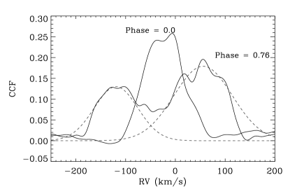
Figure 2: Cross-correlation profiles (CCF) of the observed spectra with a template spectrum at two different orbital phases (solid curves). The dashed curve is a double-Gaussian fit at phase 0.76, obtained by fitting the upper 50% of the profiles.

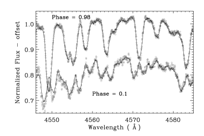
Figure 3: Fit of the observed spectra by KOREL disentangling. The circles are the observations while the solid curves are the superimposed RV Doppler-shifted disentangled spectra (y-shifted for clarity).

3.5 Disentangling of spectra

KOREL is a FORTRAN based code that fits time series of observed spectra of a multiple stellar system in the Fourier wavelength domain, to decompose them into mean spectra of each component, and simultaneously finds the best estimate of the orbital parameters (Hadrava 1995). It also calculates RVs of all components by fitting each exposure as a superposition of the disentangled spectra. We use the recent version KOREL08 to find RVs with a sub-pixel precision (cf. Hadrava 2009).

As the spectral lines are broad and hence more likely blended with nearby lines, we carefully chose several wavelength regions where the orbital motion could be clearly observed. We have chosen regions containing different numbers of spectral lines: 4537–4595Å, 4931–4995Å, 4975–5038Å, 5300–5368Å, 5506–5577Å, and 6340–6357Å. We only used the data from FEROS, FIES, and FOCES because these provided the highest SNR as well as allowing sufficient spectral resolution for the combined data set.

Each spectral region was disentangled independently converging the following parameters: periastron epoch, eccentricity $e$, longitude of periastron $\Omega$, semi-amplitude of the radial velocity curve of the primary component $K_{A}$, and mass ratio $q\equiv K_{A}/K_{B}$ (=$M_{B}/M_{A}$). The orbital period $\Pi$ was held fixed to the constant 5.71098 days (MR05), because the spectral data can not improve this previous determination. Also, note that the systemic velocity $\gamma$ is not obtained from disentangling, because KOREL does not use any spectrum template. To determine the optimal orbital parameters, we inspected both the residual value of the KOREL fit as well as the extracted RV curves. However, broad spectral profiles enlarge the range of acceptable orbital values considered as “good fits”. For each of the spectral regions we obtain a set of RV measurements.

Fig. 3 shows the observed spectra (circles) for the spectral region 4546–4585 Å at orbital phases 0.98 (eclipse) and 0.1 (separated). The solid curve is the sum of the individual disentangled primary and secondary spectra, but x-shifted by their RVs at the appropriate orbital phase and, for maintaining clarity, we also vertically shift the phase = 0.1 spectrum.

Table 2: Spectroscopic orbital solutions based on fitting the radial velocities obtained using different data fitting methods, explained in Sect. 3.

	LSD+GAU	LSD+MM	IRAFfull	IRAF	KOREL	I09
$e$	0.27 (0.02)	0.28 (0.04)	0.27 (0.08)	0.27 (0.05)	0.29 (0.01)	0.25 (0.04)
$\Omega$ (∘)	83.6 (2.0)	78.6 (4.9)	80.5 (9.9)	81.1 (6.0)	76.8 (5.0)	46.7 (7.6)
$T_{0}$ (days)	–0.07 (0.05)	–0.06 (0.17)	–0.07 (0.41)	–0.12 (0.22)	-0.1 (0.2)	–0.44 (0.27)
$\gamma$ (km s-1)	–28.1 (0.4)	–30.0 (1.5)	–29.2 (2.8)	–29.2 (1.7)	–	–27.8 (2.3)
$K_{A}$ (km s-1)	88.2 (0.9)	84.3 (2.7)	84.3 (5.1)	91.9 (3.2)	87.3 (3.5)	85.5 (3.9)
$K_{B}$ (km s-1)	94.6 (1.1)	90.7 (2.8)	91.2 (5.6)	100.5 (3.8)	93.0 (4.0)	95.9 (4.5)
M${}_{A}\sin^{3}i$ (M⊙)	1.67 (0.12)	1.45 (0.11)	1.48 (0.23)	1.96 (0.19)	1.58 (0.15)	1.69 (0.18)
M${}_{B}\sin^{3}i$ (M⊙)	1.55 (0.11)	1.35 (0.11)	1.37 (0.21)	1.79 (0.16)	1.48 (0.13)	1.51 (0.16)
$\chi^{2}_{R}$	2.7		0.04	0.07	0.86	0.7

4 Orbital parameters based on RVs

From each of the methods explained in Sect. 3 we obtain a set of RV measurements. In order to obtain the orbital parameters of the binary system we fit each set separately using the standard radial velocity equations. The results are summarised in Table 2, where the orbital period is fixed at 5.70198 days (MR05), $T_{0}$ is the offset in days from the defined primary minimum, and $\chi^{2}_{R}$ is the reduced $\chi^{2}$ value. For the LSD+MM method we have SNR values instead of observational error measurements, so the $\chi^{2}_{R}$ value is not comparable with the other methods. The uncertainties quoted are the standard formal uncertainties calculated from the fitted parameters and using the observational errors given for each RV data point. The results for KOREL are obtained by weight combining all of the RV measurements from the individual spectral profiles, and subsequently fitting using the standard equations, while the uncertainties reflect the variation in the fitted orbital parameters from the different spectral regions. These are the RV data that were later used for the simultaneous photometric and spectroscopic analysis (Sect. 5). We also analysed the published RVs from I09, who had used standard IRAF procedures to determine these. The results are given under heading I09.

We define the primary component as the more massive star. The primary is the star that shows the deeper LSD or CCF profiles as well as the line-profile variations due to pulsations (see Sect. 9).

Fig. 4 shows the phased radial velocity data from each of the methods: LSD+MM (crosses), IRAF (diamonds), LSD+GAU (squares), and KOREL (triangles — we have included a weighted average $\gamma$ shift of -28.02 km s^-1 for clarity). The dotted curve shows the radial velocity solution given by the parameters using KOREL and shifting it vertically by $\gamma$.

All of the methods presented return values of $e$, $\Omega$, $T_{0}$ and $\gamma$ consistent with each other (Table 2). There is, however, a variation among the fitted values of $K_{A}$ and $K_{B}$. This is due to the sensitivity of the various methods used to extract the radial velocities. Two possible reasons that affect the determination of the RVs are (1) the effect of the pulsations on the spectral profiles, and (2) line-broadening due to rotation making it difficult to accurately determine RVs (especially at conjunction).

If we inspect Fig. 1 we see that the double-Gaussian function cannot correctly reproduce the shape of the LSD profile. In fact, due to the wiggles or variations in the line, the actual center of the Gaussian could be shifted slightly to the right or the left. We have highlighted the center positions derived using the LSD+GAU and LSD+MM methods with the continuous and dashed vertical lines. In this figure it can also be seen that the latter method is sensitive to the minima of the deepest variations in both the primary and secondary profiles. In this case, it results in smaller absolute values of the RVs than the former method. By inspecting these profiles by eye, it is very difficult to distinguish which is the true orbital motion RV.

For phases between $\sim$0.35 and 0.7 we begin to see blending of the component profiles using both CCFs and LSD methods. Hence the resulting RVs between these phases will not be as accurate. For example, the deviations of the RVs using the LSD+MM method from the fitted RV curve in Fig. 4 are explained most likely by the sensitivity of this method to the deformations in the line profiles induced by pulsations.

In Fig. 2 we show the CCF calculated using IRAF procedures at two different orbital phases. For phase = 0.76 we have also plotted the Gaussian fits. Again, it is difficult to extract an accurate RV value because the lines are so broad and due to the variations (wiggles) in the CCFs. These values were obtained using the upper 50% of the CCF (although we draw the full analytical profile).

By inspecting the profiles of all of the available spectra (and CCFs or LSDs) it is not possible to distinguish between shifts of a few km s^-1, and it is these shifts that cause the differences in the fitted values of $K_{A}$ and $K_{B}$ of $\sim$6 km s^-1 shown in Table 2.

The last method used to extract the RVs was KOREL. We choose this as the best solution because it is robust against broadened/blended lines, it simultaneously fits the orbital solution (comparing all of the spectra at the same time), and it is independent of spectral templates. These are the RVs that are subsequently used for the simultaneous photometric and spectroscopic light curve fitting.

Figure 4: Phased radial velocity solution (dotted curve) obtained using the parameters from Table 2 under the column heading KOREL. The RVs obtained by the individual methods are also shown. The dashed lines delimit orbital phase at 0 and 1.

5 Combined analysis of photometric and spectroscopic data

In order to obtain a consistent photometric and RV solution for this system, we combine the RV data with an extensive photometric data set (MR05). We include photometry from some more recent (2005 and 2007) observational campaigns with the twin Danish 6-channel $uvby\beta$ photometer at the 1.5m and the 0.9m telescopes at San Pedro Martír, and Sierra Nevada Observatories (data reduced in the same manner as MR05). We also include photometric data from the P7 photometer mounted on the Flemish Mercator telescope at the Roque de los Muchachos Observatory (see Rufener 1964, 1985 for reduction procedure). In total there are more than 4000 photometric measurements obtained in each of the four Strömgren filters, spanning more than 3700 days, and 70 out-of-eclipse data points in the Geneva UBB₁B₂VV₁ filter system. We used PHOEBE (PHysics Of Eclipsing BinariEs) (version 0.31a; Prša & Zwitter 2005) and FOTEL (Hadrava 1990) to model these data, however the latter was used mainly to confirm the results. PHOEBE is a user-friendly software based on the Wilson-Devinney (WD) code (2007 v. of Wilson & Devinney 1971).

5.1 Photometric Indices

Using out-of-eclipse measurements, we calculated the Strömgren indices. We obtain $(b-y)=0.262$ mag, $m1=0.134$ mag, and $c1=1.058$ mag. The de-reddenned indices were obtained using the method described in Philip et al. (1976), these are $E(b-y)$ = 0.158 mag, $(b-y)_{0}$ = 0.104 mag, $m_{0}$ = 0.184 mag, and $c_{0}$ = 1.026 mag. If we compare these values to Crawford (1979) we obtain spectral type A6V or A7V. These values correspond to a single star with a mass range of between 1.7 and 1.9 M_⊙  and a $T_{\rm eff}$ of between 7400–8100 K. The value of $(b-y)_{0}$ during the primary eclipse is 0.105 mag, practically the same value as the out-of-eclipse value. This implies that the temperatures of both stars are very similar, consistent with the estimated effective temperature ratio ($T_{B}/T_{A}$) of 1.05 from MR05.

5.2 PHOEBE

We started our fitting by varying $T_{\rm effB}$ between = 8000 and 8250 K. The value of $T_{\rm effA}=7500$ (or 7750) K is fixed, according to the effective temperature ratio of 1.05 (MR05) (and in agreement with the results from Sect. 7). We also adopted as starting spectroscopic values those given in Table 2 and the results from MR05 ($e$ = 0.24, $i$ = 73^∘, and $q$ = 0.90). We searched for the best solution by using iteratively as free parameters: the luminosity of the primary component $L_{A}$, separation $a$, $q$, $e$, $\Omega$, $i$, and $\gamma$. The radii, masses, and secondary luminosity are subsequently derived from these values.

We modelled the stars as a detached system assuming a radiative albedo for both stars equal to 1 and gravity darkening values of g_A = g_B = 1. We also attempted to model the data using the semi-detached configuration, however, most of the parameters did not converge. The model parameters from the best fit are given in Table 3. The errors are derived using PHOEBE. The velocities $v\sin i$ are determined from spectroscopy (see Sect. 8) allowing the derivation of the rotational periods $P_{\rm rot}$.

Table 3: Component and orbital results from simultaneous photometric and velocity light curve fitting with PHOEBE.

	Primary	Secondary
M (M⊙)	1.78 (0.24)	1.70 (0.22)
L (L⊙)	52.42 (2.85)	22.23 (1.33)
$T_{\rm eff}$(K)	7,750	8,250
R (R⊙)	4.03 (0.11)	2.37 (0.07)
$\log g$	3.48 (0.08)	3.92 (0.08)
$v\sin i$ (km s-1)	78 (3)	74 (4)
$P_{\rm rot}$ (days)	2.50 (0.10)	1.55 (0.09)
$e$	0.283 (0.001)
$\Omega(^{\circ})$	90.6 (0.06)
$a$ (R⊙)	20.32 (0.06)
$q=K_{A}/K_{B}$	0.96 (0.001)
$i$ (o)	73.2 (0.6)

6 Disentangling of spectra

The disentangled spectra were obtained by imposing the orbital solution from KOREL shown in Table 2. The used version of KOREL is limited in resolution to 4000 points. However, in most cases it was quicker and more stable to work on 2000 points at a time, over wavelength regions of about 100 Å. For this we had to rebin the spectra at the appropriate resolution and carefully choose the endpoints of the regions where there was continuum, while also ensuring that overlapping spectral regions are present to facilitate the merging of all of the wavelength regions.

We attempted to disentangle the spectra in the wavelength range from 4600 to 5800 Å because this region is most sensitive to abundances. However, we only obtained reliable results for $\sim$100Å-length spectral regions between 4976–5627 Å. Unfortunately, this implies that a spectroscopic determination of $T_{\rm eff}$ from the Balmer lines is not possible from the disentangled spectra: a better orbital phase coverage and higher SNR spectra are needed in order to disentangle these regions correctly.

Spectra from binary systems normalised to 1 contain no information about the relative light contributions of each of the individual spectra. We used the literature values from I09 ($L_{A}$ = 0.61 and $L_{B}$ = 0.39 where $L_{A}+L_{B}=1$), and the fitted luminosities given by our composite photometric and spectroscopic analysis ($L_{A}$ = 0.69 and $L_{B}$ = 0.31, Sect. 5) to obtain the fractional contributions to the total light. We shifted the output spectra to continuum 0, scaled the individual spectra by their corresponding fractional luminosity, and shifted the spectra again to 1 to obtain the disentangled individual spectra.

7 Spectroscopic determination of $T_{\rm eff}$

Once the spectra were disentangled, we proceeded to obtain the LSD profiles of the individual disentangled spectra (Sect. 3.1), in order to estimate $T_{\rm eff}$ and $\log g$. We calculated the LSD profiles using a range of templates spanning $T_{\rm eff}$ (7250–8500 K) and $\log g$ (3.5–4.5), and identified the best values as those that produced the best LSD profiles (smoothest and most symmetric). Using the luminosity ratios obtained, $T_{\rm eff}$ of the primary was best fit with a template spectrum of 7500 K with $\log g=4.0$. The secondary was best fit with a hotter temperature of 8000 – 8250 K and $\log g$ = 3.5, although $\log g=4.0$ was also a good fit. In general, the results are much less sensitive to the value of $\log g$ than to changes in $T_{\rm eff}$.

As the disentangled renormalised spectra depend on the assumed luminosity ratio of both components, we performed a few tests to investigate how these results depend on this imposed value. We scaled each of the disentangled spectra arbitrarily, and proceeded to identify the best $T_{\rm eff}$ for each of the “synthetic” spectra in the same manner as above (as double-blind tests). The results were again quite insensitive to the value of $\log g$, while the derived values of $T_{\rm eff}$ were consistent with results of 7500–7750 K for the primary, and 8000–8250 K for the secondary. This test showed that the identified $T_{\rm eff}$ were not obtained from the imposed luminosity ratio of the stars, but rather the shape of the spectra. MR05 obtained an effective temperature ratio ($T_{B}/T_{A}$) of $\sim$ 1.05 (secondary/primary), in agreement with our result, while I09 obtained a hotter temperature for the primary component than for the secondary ($T_{B}/T_{A}\sim 0.96$).

We also directly compared composite rotationally-broadened RV- and $\gamma$-shifted Kurucz synthetic spectra to the best SNR observations near maximum elongation phase. We used templates spanning temperatures of 7000 - 8500 K and $\log g$ of 3.5 - 4.5 dex. Figure 5 shows the observations (grey) compared to various templates (black) for the temperature-sensitive H-$\beta$ line. As shown in this figure, the best fitted temperatures are 7500-7750 and 8000-8250 K for primary and secondary star, respectively. (The $\log g$ values used are 3.5).

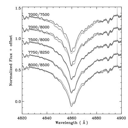
Figure 5: Composite rotationally broadened RV- and $\gamma$-shifted spectral templates (black) with observations (grey) for various combinations of $T_{\rm eff}$ (K) for the primary and secondary components.

8 Abundance Analysis

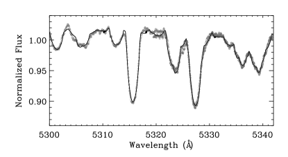
Figure 6: The disentangled observed primary spectrum (open circles), and the theoretical fitted spectrum (solid) obtained using the abundances from Table 4.

Table 4: The abundances of chemical elements for the primary and secondary stars.

Atomic	No. lines used	Primary	Secondary	Sun
No.	Prim./Sec.
6	4/2	8.45 (0.15)	8.78 (0.28)	8.39
8	1/1	8.89 (0.13)	8.82 (0.13)	8.66
11	1/–	6.21 (0.08)		6.17
12	2/2	7.35 (0.16)	8.37 (0.30)	7.53
13	1/–	6.17 (0.38)		6.37
14	2/2	7.81 (0.21)	7.91 (0.12)	7.51
16	1/–	6.67 (0.21)		7.14
20	4/4	6.28 (0.18)	6.92 (0.23)	6.31
21	2/2	3.12 (0.10)	3.89 (0.26)	3.17
22	9/9	4.90 (0.18)	5.38 (0.21)	4.90
24	4/5	5.81 (0.14)	6.31 (0.13)	5.64
26	19/20	7.17 (0.21)	7.84 (0.19)	7.45
27	1/–	5.57 (0.02)		4.92
28	6/9	6.13 (0.18)	6.89 (0.22)	6.23
39	2/2	2.72 (0.20)	2.78 (0.17)	2.21
40	–/1		3.20 (0.08)	2.58

We determined the abundances of both components using the disentangled renormalised spectra. We compared the results with both values of luminosity fraction, and the final abundances varied slightly, but within the quoted errors. Our analysis follows the methodology presented in Niemczura & Połubek (2006) and relies on an efficient spectral synthesis based on a least-squares optimization algorithm (Bevington 1969, Takeda 1995). This method allows the simultaneous determination of various parameters associated with stellar spectra and consists of minimizing the deviation between the theoretical flux distribution and the observed one.

The atmospheric models used for the synthethic spectra determination were computed with the line-blanketed LTE ATLAS9 code (Kurucz 1993), which handles line opacity with the opacity distribution function. The synthetic spectra were computed with the SYNTHE code (Kurucz 1993). Both codes were ported to GNU/Linux by Sbordone (2005). The identification of stellar lines and the abundance analysis were performed on a line list we constructed based on VALD data (Kupka et al. 2000 and references therein).

The shape of the synthetic spectrum depends on the stellar parameters such as $T_{\rm eff}$, $\log g$, $v\sin i$, microturbulence $\xi$, RV and relative abundances of the elements. The effective temperature and surface gravity were not determined during the iteration process but were considered as fixed input ones (T_eff = 7500/8000 and $\log g$= 4.0/4.0 for primary/secondary components), while $\xi$ = 2 km s^-1 was adopted. All of the other above-mentioned parameters can be determined simultaneously because they produce detectable and different spectral signatures. The theoretical spectrum was fitted to the normalised observed one in small regions, until the results converged. The obtained chemical element abundances, relevant errors with the adopted solar abundances (Grevesse et al. 2007) are given in Table 4. The errors are calculated as $\sigma_{\rm Tot}=[\sigma_{\rm ab}^{2}+\sigma_{T_{\rm eff}}^{2}+\sigma_{\log g}^{2}]^{1/2}$ where $\sigma_{\rm ab}$ is the standard deviation of the individual element abundance, $\sigma_{T_{\rm eff}}$ and $\sigma_{\log g}$ denote the variation of abundance for $\Delta T_{\rm eff}\pm 250$ K and $\Delta\log g\pm 0.2$. For those elements where only one line was used to estimate the abundance, the error is $(\sigma_{T_{\rm eff}}^{2}+\sigma_{\log g}^{2})^{1/2}$.

Apart from the errors in $T_{\rm eff}$ and $\log g$, several systematic errors are likely affecting the derived abundances. For example, fixing $\xi$, the restriction of the disentangling technique to the spectral range of 4976–5672 Å  and the imposed luminosity ratio all contribute to these sytematic errors. In addition to this, the adopted atmospheric models and the atomic data (in particular the oscillator strengths) also contribute. We are also not taking NLTE effects into account, which are crucial for a number of spectral lines of several elements (see e.g. Asplund 2005; Fabbian et al. 2006, 2009). However, we have estimated that for the neutral C lines used here, the NLTE corrections are negligible (private comm. Fabbian). Moreover, even for other chemical elements we can safely assume that the differential NLTE effects between the primary and secondary stars are small and hence can not explain the differences for some of the elements between the two stars.

Figure 6 shows a region of the primary disentangled spectrum (circles) and the theoretical fitting to it (solid curve) which is obtained using the abundances from Table 4. The chemical composition of the primary star is slightly sub-solar, judging from the Fe content, while the secondary star shows enhanced abundances (see Fig. 7). The derived rotational velocities are $v\sin i$ = 78 $\pm$ 3 km s^-1and 74 $\pm$ 4 km s^-1for primary and secondary component respectively, based on a comparison between the spectra with broadened theoretical profiles. Coupling these values with the results for R_⊙ and $i$ from Table 3, we derive the following rotational periods: $P_{\rm rot,A}=2.50\pm 0.10$ days for the primary star and $P_{\rm rot,B}=1.55\pm 0.09$ days for the secondary.

We have also performed a comparison abundance analysis based on a detailed line abundance approach using the MOOG code. The full procedure is described in Arellano Ferro et al. (2001) and Giridhar & Arellano Ferro (2005). The number of elements analysed is smaller than those shown in Table 4, but the overall Fe abundance and the indication that the secondary component is iron rich is consistent with our previous result. This analysis yielded the best results when $T_{\rm eff}$ of 7750 and 8000 K, and $\log g$ of 3.0 and 3.5 were adopted for primary and secondary, respectively.

9 Discussion

9.1 Orbital and System parameters

From the spectroscopic and the combined photometric and spectroscopic analysis we obtain system parameters that are in agreement: $e=0.29$, $\Omega\sim 80^{\circ}$ and $T_{0}\simeq-0.1$ (this result is compatible with $T_{0}\simeq 0.0$ taking the error into account, and this value indicates that the resulting offset in days from eclipse/conjunction coincides with the input value from MR05). When we compare our results with the only other published system parameters by I09, we find that I09 obtain from their combined photometric and spectroscopic analysis a lower value of the eccentricity (e=0.19). When we fit their data using our RV solution method, we obtain $e=0.25$, $\Omega\simeq 47^{\circ}$ and $T_{0}=-0.4$. However, when we use $\Omega=80^{\circ}$ and $T_{0}=-0.1$ as fixed values we obtain a $\chi^{2}$ value that increases by less than 1 (i.e. less than 1$\sigma$), indicating that this solution is also plausible with their data. The average $\gamma=-28.0$ km s^-1 is consistent with the cluster radial velocity of –25.0 km s^-1(Valitova et al. 1990): providing extra evidence of the system’s membership to the cluster.

The derived value of $i=73^{\circ}$ indicates that if we aim to determine precise masses, we must accurately determine the values of $K_{A}$ and $K_{B}$. Given that we obtain a range of about 6 km s^-1 in both $K_{A}$ and $K_{B}$ this implies that the minimum mass error is already on the order of a few tenths (if we just use the analytical calculation and the inferred inclination). The resulting values for $M\sin^{3}i$ are listed in Table 2, where it can be seen that the variation is of the order of 0.3 M_⊙ (all however within 3$\sigma$ of each other). In Sect. 4 we already discussed the sensitivity of each of the methods in obtaining the RVs, and we would like to point out the difficulty of attempting to model the type of stellar system considered here. What hampers the precise determination of the RVs of each component is the significant broadening of the spectral line profiles due to the rotation of both stellar components, and the superimposed pulsations.

The largest differences in the results come from using the same method (IRAF) but choosing a different cut-off region in the CCF profiles to model. While the two-Gaussian function did not show reasonable results for IRAF_FULL, an adequate 3-Gaussian fitting to the CCF seemed to fit the profile better indeed. This third low amplitude component could be a sign of a third body in the orbit.

When combining the photometric and spectroscopic data (Sect.5) it was difficult to arrive at a solution that (iteratively) converged using the parameters listed in Table 3 as free parameters. This is most likely a result of the rapid rotation causing surface temperature variations at different latitudes (sometimes a difference of up to 1,500 K for very rapid rotation). The photometric light curve is distorted due to these variations, and these effects are not taken into account in the modeling (the assumption with PHOEBE is that the star rotates as a rigid body, without differential rotation). Additionally, one of the components has visible photometric variability on time scales of $\sim$1 hour (MR05, Amado et al. 2006, Costa et al. 2007), and although the light curves were binned to reduce the effects of pulsation, there are nonetheless effects that can not be eliminated, such as those during eclipse.

We obtain component masses of 1.78 $\pm$ 0.24 and $1.70$ $\pm$ 0.22 M_⊙ for primary and secondary stars respectively, values that are lower by $\sim 0.2$ M_⊙ than those from I09 (2.06 and 1.87 M_⊙). Our results are consistent with the values obtained by Mermillod & Mayor (1990) who, through a study of red giants, determined the main sequence (MS) turn-off mass of IC 4756 to be between 1.8 and 1.9 M_⊙. This would also be consistent with the hypothesis of the more massive component beginning to turn off the MS, while also implying that the secondary star is slightly hotter than the primary.

We obtain primary and secondary radius of 4.03 $\pm$ 0.11 and 2.37 $\pm$ 0.07 R_⊙, respectively, luminosities of 52.42 $\pm$ 2.85 and 22.23 $\pm$ 1.33 L_⊙, and $\log g$ values of 3.48$\pm$0.08 and 3.92$\pm$0.08 (see Table 3). These values are lower than those quoted by I09, due primarily to the lower fitted masses we obtain.

We finally fixed the values of $T_{\rm eff}$ at 7500–7750 and 8000–8250 K respectively. This choice is justified by the following reasons: (a) at an earlier stage during this work, modeling the photometric light curve produced similar answers (7,560 and 8,030 K) while fixing various other parameters, (b) modeling the light curve while fixing the $T_{\rm eff}$ at other values results in worse fits or non-convergence, (c) the photometric Strömgren indices are consistent with these ranges of values (Sect. 5), and (d) the spectroscopic determination of $T_{\rm eff}$ from the LSD profiles and synthetic spectra also arrives at these values (Sect.7).

The primary (hotter and more massive) star is the pulsating component that clearly shows line-profile variations. Our data do not allow us to determine if the secondary component is also pulsating as the SNR is too low to detect low-amplitude variability, if any. The results in Sect. 5 and Table 3 do not discard the possibility of two pulsating components — both stars lie within the $\delta$ Scuti instability strip close to the blue edge (see Fig. 13 in Pamyatnykh 2000).

We have explored various forms of determining the RVs from the 70 spectra collected between 2005 and 2007 as well as using photometric observations spanning over 3000 days. Taking into account the uncertainties, our results are consistent with the I09 ones, however, apart from the RV dataset derived with the IRAF method, we obtained lower masses and this would imply a downward revision of these values to 1.8 and 1.7 M_⊙.

9.2 Abundances

The resulting abundances given in Table 4 indicate for the primary component a sub-solar metal value of [Fe/H] $=-0.28$ consistent with the values of –0.15 and –0.22 determined for the cluster IC 4756 derived from samples of F-G single star cluster members by Jacobson et al. (2007) and Thogersen et al. (1993), respectively. The results of I09 also showed that this system component’s global parameters fitted better to a sub-solar metallicity evolutionary track ($Z\sim 0.008$, where $Z$ is the initial metal mass fraction). For HD 172189 we obtain the following abundances (primary/secondary): [Na/Fe] = +0.03/–, [Al/Fe] = +0.00/–, [Si/Fe] = +0.08/+0.00, [Ca/Fe] = +0.03/+0.04, and [Ni/Fe] = +0.02/+0.04. These values are consistent with those of IC 4756 according to Jacobson et al. (2007). However, their values are higher than ours by up to $\sim$0.3 dex (they quote +0.6, +0.3, +0.34, +0.07, +0.08, respectively). This could be in part due to the adopted $\log-gf$ values (Jacobson et al. 2007).

Figure 7: Abundances of the primary (filled circles) and secondary (open circles) stars compared to the adopted solar values. The bars represent errors of $\pm 1\sigma$.

The abundances relative to hydrogen for the primary star are: $[{\rm Fe/H}]=-0.28$, [Si/H] $=+0.3$, [Ca/H] $=-0.03$, [Ni/H] $=-0.10$, [Na/H] $=+0.04$. These values are comparable to Jacobson et al. (2007), who obtained –0.15, +0.19, –0.08, –0.07, +0.2 for IC 4756. The results for the secondary star are [Fe/H] = +0.4, [Si/H] = +0.4, [Ca/H] = +0.6, [Ni/H] = +0.6, on average $\sim$0.5 dex higher than the primary star, resulting in enhanced abundances compared to the Sun. Fig. 7 shows the abundances relative to the solar ones. The enhanced abundances of the secondary star could also be an effect of modeling a spectrum with an inadequate normalisation from the disentangling. Higher SNR disentangled spectra resulting from the full orbital phase coverage would be able to confirm these different abundances.

10 Conclusions

We analysed a set of spectroscopic data obtained between 2005 and 2007 with the aim of determining the absolute component masses, radii, luminosities, and effective temperatures of the system, as well as undertaking the first abundance analysis of the HD 172189 disentangled spectra. From a combined photometric and radial velocity analysis, we derive for the primary and secondary stars, respectively, masses of 1.78$\pm$0.24 and 1.70$\pm$0.22 M_⊙ radii of 4.03$\pm$0.11 and 2.37$\pm$0.07 R_⊙, luminosities of 52.42$\pm$2.85 and 22.23$\pm$1.33 L_⊙, and $\log g$ of 3.48$\pm$0.08 and 3.92$\pm$0.08 dex. The analysis of the spectra indicates a $T_{\rm eff}$ of 7600$\pm$150 K and 8100$\pm$150 K. From the RV data, we derive the system orbital parameters: $e=0.29\pm 0.02$, $\Omega=77^{\circ}\pm 5$ (from KOREL), and $\gamma=-28.02\pm 0.37$ km s^-1 (from other RV methods), and from the photometric data $i=73.2^{\circ}\pm 0.6$ and $a=20.32\pm 0.06$ R_⊙. The spectroscopic data also confirm the orbital period of the system: 5.70198 days, as derived by MR05. We also obtain a spectral type of A6V-A7V based on Strömgren photometry.

We applied four methods to calculate the RVs and obtained different results for each. We subsequently showed the limitations of each technique for analysing a system with two rapidly-rotating components, one of these having the additional complications of showing significant profile-variations due to pulsations. Obtaining higher SNR spectra with continuous phase coverage would help to determine the systematic differences between each of the methods.

We have disentangled the spectra of both components and determined the rotational velocities: $v\sin i$ = 78$\pm 3$ km s^-1 and 74$\pm$4 km s^-1. Coupling these values with the results for R_⊙ and $i$ we obtain rotational periods $P_{\rm rot,A}=2.50\pm 0.10$ days and $P_{\rm rot,B}=1.55\pm 0.09$ days. We subsequently derived a metallicity of [Fe/H] = –0.28 dex and abundances of [Si/H] = +0.3, [Ca/H] = –0.03, [Ni/H] = –0.10 and [Na/H] = +0.04 for the primary star. These are consistent with the results published for the cluster IC 4756 by Jacobson et al. (2007). The sub-solar metallicity is also consistent with the findings from I09.

The rapid rotation of both components, the non-synchronous rotation (based on the orbital period), the eccentricity, and the likely membership of IC 4756 suggests that the system is still detached. Based on the inferred age of the system of 0.8–0.9 Gyr (Alcaino 1965, Mermillod & Mayor 1990) we estimate that the 1.8 M_⊙ primary star is moving towards the end of its MS lifetime, when it begins to cool down and increase in luminosity. Mermillod & Mayor (1990) also determine that the main sequence turn-off mass for this cluster is 1.8–1.9 M_⊙, which agrees with this hypothesis.

In order to study the oscillations of the primary star, recently CoRot (Baglin et al 2006a,b, Michel et al. 2008) observed HD 172189 as a primary asteroseismic target. Our analysis of this data has given a thorough insight into the nature of this object, and hence forms a solid foundation for the subsequent asteroseismic analysis. We look forward to the unravelling of the mysteries associated with this object, and to learning about the effects of rotation on the interior structure of the star from the pulsation frequencies.

- (1) Aerts, C., De Pauw, M., & Waelkens, C. 1992, A&A, 266, 294
- Amado et al. (2006) Amado, P. J., Martín-Ruíz, S., Suárez, J. C., Arellano Ferro, A., Moya, A., Ribas, I., & Poretti, E. 2006, Ap&SS, 304, 173
- Alcaino (1965) Alcaino, G. 1965, Lowell Observatory Bulletin, 6, 167
- (4) Arellano Ferro, A., Sunetra Giridhar, P. Mathias. 2001, A&A, 368, 250-268
- Asplund (2005) Asplund, M. 2005, ARA&A, 43, 481
- (6) Baglin, A., et al. 2006a, 36th COSPAR Scientific Assembly, 36, 3749
- Baglin et al. (2006) Baglin, A., Auvergne, M., Barge, P., Deleuil, M., Catala, C., Michel, E., Weiss, W., & The COROT Team 2006b, ESA Special Publication, 1306, 33
- Bevington (1969) Bevington, P. R. 1969, New York: McGraw-Hill, 1969,
- (9) Briggs, K. R., Pye, J. P., Jeffries, R. D., & Totten, E. J. 2000, MNRAS, 319, 826
- Brun et al. (2004) Brun, A. S., Browning, M., & Toomre, J. 2004, Stellar Rotation, 215, 388
- (11) Costa, J. E. S., et al. 2007, A&A, 468, 637
- (12) Cox, A. 2000, Allen’s Astrophysical Quantities, 4th Ed., AIP
- (13) Crawford D.L., 1979, AJ 84, 1858
- (14) Donati, J.-F., Semel, M., Carter, B.D., Rees, D. E., & Collier Cameron, A. 1997, MNRAS, 291, 658
- (15) Donati, J.-F., Catala, C., Wade, G.A., et al. 1999, A&AS, 134, 149
- Dzěrvitis (1987) Dzěrvitis, U. 1987, Nauchnye Informatsii, 63, 36
- Fabbian et al. (2006) Fabbian, D., Asplund, M., Carlsson, M., & Kiselman, D. 2006, A&A, 458, 899
- Fabbian et al. (2009) Fabbian, D., Asplund, M., Barklem, P. S., Carlsson, M., & Kiselman, D. 2009, arXiv:0902.4472
- Featherstone et al. (2007) Featherstone, N., Browning, M. K., Brun, A. S., & Toomre, J. 2007, Bulletin of the American Astronomical Society, 38, 117
- (20) Giridhar, S. & Arellano Ferro, A. 2005, A&A, 443, 297-308
- (21) Graff, K. 1923, Astronomische Nachrichten, 217, 311
- (22) Grevesse, N., Asplund, M., & Sauval, A. J. 2007, Space Science Reviews, 130, 105
- (23) Hadrava, P. 1990, Contr. Astron. Obs. Skal. Pl., 20, 23
- (24) Hadrava, P. 1995, A&AS 114, 393
- (25) Hadrava, P. 2009, A&A 494, 399
- Herzog et al. (1975) Herzog, A. D., Sanders, W. L., & Seggewiss, W. 1975, A&AS, 19, 211
- (27) Ibanoǧlu, C., et al. 2009 (I09), , 392, 757
- (28) Jacobson, H. R., Friel, E. D., & Pilachowski, C. A. 2007, AJ, 134, 1216
- Kopff (1943) Kopff, E. 1943, Astronomische Nachrichten, 274, 69
- (30) Kupka, F., Piskunov, N., Ryabchikova, T. A., Stempels, H. C., & Weiss, W. W. 1999, A&AS, 138, 119
- (31) Kupka, F.G., Ryabchikova, T.A., Piskunov, N.E., et al., 2000, BaltA, 9, 590
- Kurucz (1993) Kurucz, R. L. 1993, Kurucz CD-ROM, Cambridge, MA: Smithsonian Astrophysical Observatory, —c1993, December 4, 1993
- Luck (1994) Luck, R. E. 1994, ApJS, 91, 309
- Martin (2003) Martin, S. 2003, Interplay of Periodic, Cyclic and Stochastic Variability in Selected Areas of the H-R Diagram, 292, 59
- (35) Martín-Ruiz S., et al., 2005 (MR05), A&A 440, 711
- Mermilliod & Mayor (1990) Mermilliod, J.-C., & Mayor, M. 1990, A&A, 237, 61
- Michel et al. (2008) Michel, E., et al. 2008, Communications in Asteroseismology, 156, 73
- Missana & Missana (1995) Missana, M., & Missana, N. 1995, AJ, 109, 1903
- (39) Niemczura, E., Połubek, G., 2006, ESASP, 624, 120
- Pamyatnykh (2000) Pamyatnykh, A. A. 2000, Delta Scuti and Related Stars, 210, 215
- (41) Philip A.G.D., Miller T.M., Relyea L.J., 1976, Dudley Observatory Report No.12, 1
- (42) Piskunov, N.E., Kupka, F., Ryabchikova, T.A, Weiss, W.W. & Jeffery, C.S. 1995, A&ASS, 112, 525
- (43) Prša A. & Zwitter T., 2005, ApJ 628, 426
- (44) Rainer, M. 2003, Analisi spettrofotometriche di stelle da usare come targets per la missione spaziale CoRoT, Laurea Thesis, Universitá degli Studi di Milano
- (45) Rufener, F. 1964, Publ. Obs. Genéve, A, 66, 413
- (46) Rufener, F. 1985, In: Hayes D. S. et al. (eds) Calibration of Fundamental Stellar Quantities, IAU Symp. 111, Reidel Publ. C., Dordrecht, p.253
- (47) Ryabchikova, T.A., Piskunov, N.E., Stempels, H.C., Kupka, F. & Weiss, W.W. 1999, Physica Scripta, 83, 162
- Schmidt (1978) Schmidt, E. G. 1978, PASP, 90, 157
- (49) Sbordone, L., 2005, MSAIS, 8, 61
- Schmidt & Forbes (1984) Schmidt, E. G., & Forbes, D. 1984, MNRAS, 208, 83
- (51) Takeda, Y., 1995, PASJ, 47, 287
- Thogersen et al. (1993) Thogersen, E. N., Friel, E. D., & Fallon, B. V. 1993, PASP, 105, 1253
- (53) Tody D., 1986, in Crawford D., ed., Instrumentation in Astronomy VI Vol. 627, The iraf data reduction and analysis system. p. 733
- (54) Uytterhoeven, K., Mathias, P., Poretti, E., et al. 2008, A&A, 489, 1213
- Valitova et al. (1990) Valitova, A. M., Rastorguev, A. S., Sementsov, V. N., & Tokovinin, A. A. 1990, Soviet Astronomy Letters, 16, 301
- Wachmann (1939) Wachmann, A. A. 1939, Spektral-Durchmusterung von Milchstrassenfeldern. Teil 1 , 1 (1939), 0
- (57) Wilson R.E. & Devinney E.J., 1971, ApJ 166, 605