Electrostatics of Graphene: Charge Distribution and Capacitance
Abstract
The distribution of net electric charge in graphene is investigated, using both a constitutive atomic charge-dipole interaction model and an approximate analytical solution to Laplace’s equation. We demonstrate a strong size dependence of the charge distributions in finite-size, infinitely-long and multi-layered rectangular graphene sheets, respectively. We found that the charge density can be naturally enhanced up to 13 times at graphene’s geometry edges. This edge charge enhancement effect becomes more significant when the length or the width of graphene increases. The charge enhancement ratio is found to follow a linear relationship with the number of layers. These results can be used to understand the newly experimentally observed electron emission, charge impurity and chemical doping phenomena in 2-dimension nanostructure.
pacs:
41.20.Cv, 81.05.UwI Introduction
Graphene is an hexagonally coordinated semi-metallic or zero-gap-semiconducting carbon layer that crystallizes in structure. Its unusual band structure Castro Neto et al. (2009); Beenakker (2008) leads to unique electronic properties such as high charge carrier mobility Hwang et al. (2007); Morozov et al. (2008); Fogler et al. (2008) and tunable electron band gap by external electromagnetic fields Son et al. (2006); Yang et al. (2007); Han et al. (2007); Castro et al. (2007); Novikov (2007); Yan et al. (2007) or by chemical doping.Duplock et al. (2004); Biel et al. (2009) These make graphene an ideal candidate for a number of applications in nanoelectronics.Westervelt (2008) Recently, it has been shown by electrostatic force microscopy experiments that electric charges can be stored in carbon nanotubes for a period of time.Paillet et al. (2005); Zdrojek et al. (2005); Jespersen and Nygard (2005) It would not be surprising if graphene exhibits similar properties, because of the large similarity in its atomic structures to that of nanotubes.Charlier et al. (2007) The investigation on electronic properties of graphene doped with net charges is of importance for understanding the charge impurities Morozov et al. (2006); Yan and Ting (2008); Rossi and Das Sarma (2008) or chemical doping Duplock et al. (2004); Biel et al. (2009) in graphene, and may as well lead to further applications in charge storages,Cui et al. (2002) sensors Robinson et al. (2008) and field-emission devices Bonard et al. (2002); Purcell et al. (2002b) based on graphene.
The question about the exact solution to the charge distribution in an arbitrary-shaped conducting surface has been raised since the theoretical basis of electromagnetism was established by J. C. Maxwell in 1873.Maxwell (1873) For graphene, the electrostatic problem of finding the charge distribution on the surface of a conducting, rectangular plate requires the solution to Laplace’s equation in the three-dimensional geometry. Unfortunately, even such a seemingly simple problem has no exact solution: The number of exact solutions in three-dimensions is still limited to specialized geometries that exhibit a great deal of symmetryJackson (1975); Morse and Feshbach (1953); Bottcher (1952). In this paper, the charge distribution was first calculated using a numerical atomic charge-dipole model. Comparisons are then made between the result of a simple, one-term variational approximation and a numerical solution, which is found to give a more accurate description of the edge atoms.
The remainder of this paper is organized as follows. In Sec. (II) we describe first our numerical method and then we demonstrate a variational approach to solve Laplace’s equation and calculate the charge distribution on a conducting rectangular plate. The results of both numerical and analytical models are compared and discussed in Sec. (III). We draw a conclusion in Sec. (IV). Mathematical details of the one-term variational approximation are summarized in the Appendix.
II Theory
II.1 Numerical method
In this work, the charge density was first calculated using a computational atomic charge-dipole model,Mayer (2007) in which each atom is modeled as a polarizable sphere with a net charge and an induced dipole . The equilibrium distribution of the charges and the induced dipoles in graphene is determined by minimizing the total electrostatic potential energy of the system
| (1) |
where is the electron affinity, and where and are the external potential and electric field, respectively. The electrostatic interacting tensors are and , which are regularized by a Gaussian distribution Wang (2009). Requiring the derivatives of with respect to and to be zero, Eq. (1) yields
| (2) |
where is the Lagrange multiplier which is related to the chemical potential of the molecule.
This numerical model is an extension of the atomic dipole interaction theories Applequist et al. (1972); Olson and Sundberg (1978); Jensen, L. (2002). It has recently been parameterized for carbon systems Mayer (2005a, b) and validated through electrostatic force microscopy charge injection experiments.Wang et al. (2008) The graphene structure is relaxed by means of an atomic energy-optimization method using the adaptive interatomic reactive empirical bond order (AIREBO) potential function,Stuart et al. (2000) which has specially been parameterized for hydrocarbon systems.Ni et al. (2002); Shenoy et al. (2008); Wang and Philippe ; Wang and Devel (2007); Wang et al. (2007)
II.2 Analytic approximation
A simple analytical approximation for the solution to Laplace’s equation is now constructed. In three physical dimensions, consider an infinitesimally thin conducting surface of rectangular shape -by- that is held to the potential , with the reference or zero potential at infinity. The rectangle lies in the plane and is the region , . We seek a solution to Laplace’s equation
| (3) |
subject to the boundary conditions
| (4) |
Based on experience with the exact solution for the two-dimensional strip problem,Morse and Feshbach (1953); Jackson (1975) we propose a one-term approximation for the (scaled) charge density
| (5) |
where the single unknown is the constant . This functional form is simply a factorization of the rectangular distribution into two edge-condition forms that apply to the classical two-dimensional strip problem. Its suitability is not a priori known, but ultimate comparison with independent moment method HarringtonMM (2009) calculations shows that it is quite respectable. The one-term Galerkin procedure in the Appendix produces an approximation for the constant
| (6) |
in terms of an integral function of Eq. (25) which is evaluated numerically. The resultant surface charge density is then
| (7) |
Integration of Eq. (7) gives the total charge
| (8) |
induced on the rectangular plate when held to the potential .
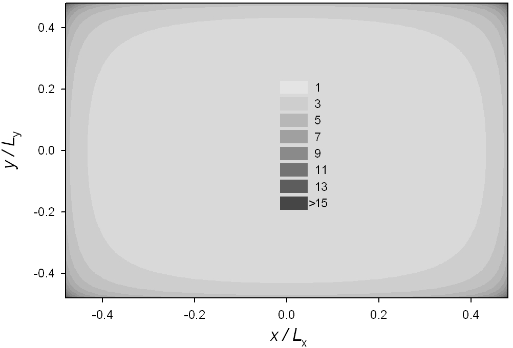
Here Fig. 1 shows the charge enhancement effect in a rectangular plate exhibited by Eq. (7). In addition to the surface charge distribution, it is instructive to also consider the capacitance , a global electrostatic characterization of the plate. In the present notation, the capacitance per unit width is
| (9) |
In the limiting case of a square, and the numerics give and the subsequent normalized capacitance is (in SI units) (pF/m), about 1.6% lower than the value (pF/m) that has been published by Goto et al.Gotoi (1992)
III Results and Discussions
III.1 Finite-size graphene
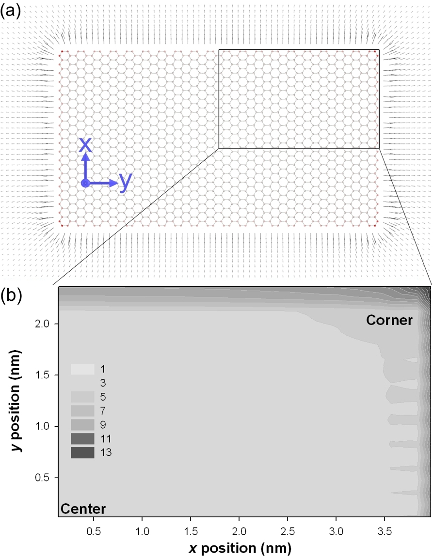
We start with mono-layered graphene which contains a quantity of net electric charge. Fig. 2 (a) shows the charge distribution in a finite-size graphene sheet, calculated using the numerical method (Sec. (II.1)). As expected, typical charge and electric field enhancement effects Wang et al. (2008) were observed near the corners and the edges. To compare these results with those predicted by Eq. (7), we show the atomic charge density in a quarter of the graphene sheet in Fig. 2 (b). Comparison between the contours of charge density in Fig. 1 and Fig. 2 (b) shows a general agreement between the analytical model and the numerical calculation. The lack of smooth trend of the contours in Fig. 2 (b) is due to the different configurations of atoms at armchair and zigzag edges and the discontinuity of our discrete model. It is found that the Eq. (7) becomes no more accurate for the atoms near the edges, because the assumption of infinitely sharp edges in the analytical solution is not valid in atomic scale. After our simulation results, the charge density (at the corner) can be enhanced up to times over that in the center of graphene. We note that the charge density can also slightly vary if the graphene is substitutionally doped by net charges (e.g. some electrons per 100 atoms), since the graphene band structure can be significantly modified in highly charged graphene.Keblinski et al. (2002) Moreover, these results also imply that the influence of induced dipoles on the charge distribution is minor.
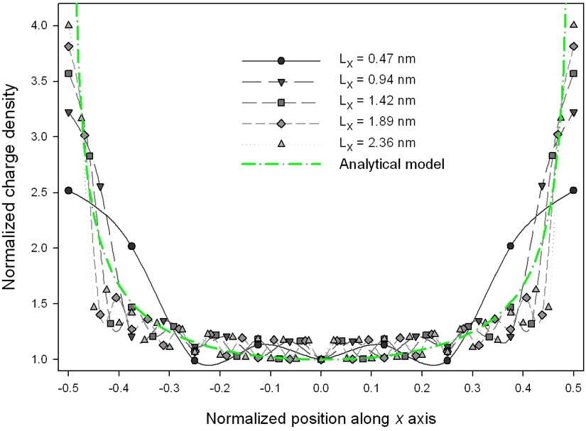
We next consider the size effect on the charge distribution. Our results show a strong dependence of the charge enhancement on the graphene length (Fig. 3). We can see that the fluctuation of the charge profile due to the edge state becomes less significant with the increasing length, and that the charge enhancement at the edges is stronger for the longer sheets. This behavior is similar to that in carbon nanotubes.Keblinski et al. (2002)
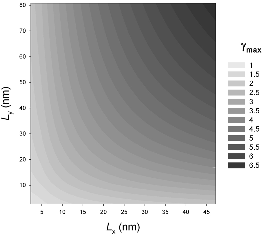
We now define the maximal charge enhancement ratio as the maximal atomic charge density normalized to the average over the whole graphene. It is one of the key parameters for the potential applications of graphene in field emission devices Bonard et al. (1998). To show a complete correlation between and the dimensions of graphene, we plot numerical calculation data of in Fig. 4 as a function of and . We can see that increases with either or , and that gets higher for . It is found that the increase of charge enhance ratio is more rapid in small size graphene sheets.
III.2 Infinitely-long graphene
To generalize our results for the graphene size usually used in experiments, it is particularly interesting to investigate the charge distribution in infinitely long graphene sheets or strips. The question of charge distribution becomes a 2D standard problem in elliptical coordinates.Morse and Feshbach (1953) The exact solution to Laplace’s equation for the strip conductor of width held to the potential gives the surface charge density
| (10) |
where is the (large) radial distance where the potential vanishes. This is the “ground” or reference surface that cannot be at infinity because of the logarithmic singularity in the 2D potential problem. Integration of the surface charge density yields the capacitance per unit length
| (11) |
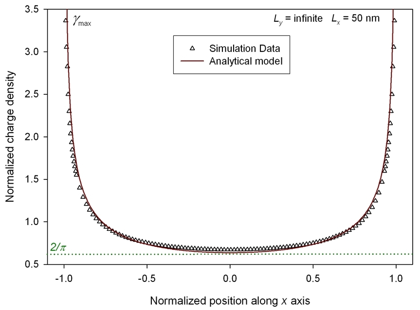
Here we show the normalized charge profile in a graphene sheet with applied periodic condition in width () direction in Fig. 5, which highlights a good agreement obtained between the numerical calculations and the analytical solution. Also, compared to Fig. 3, it can be seen that the fluctuation on the charge density curves due to the open-edge effects Liu et al. (2009) completely disappeared in the infinite-long graphene.Yang et al. (2008); Abanin et al. (2006)
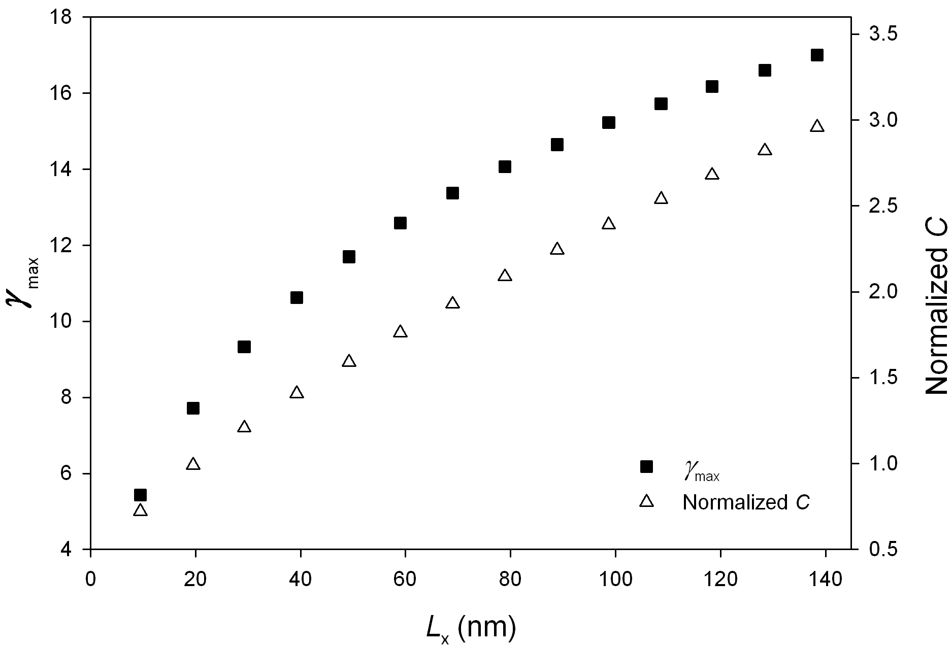
To demonstrate the size effect, we now consider the maximal charge enhancement ratio as a function of . It is shown in Fig. 6 that increases with , the shape of the curve is as predicted by the logarithm relationship proposed by Keblinski et al. Keblinski et al. (2002). Since the surface electric potential is a constant, this length dependence directly leads to the rise of the capacitance of the edge atoms. Also, we plot the normalized in Fig. 6. It can be seen that also increases with , as predicted by Eq. (11). However, it is found that the capacitance per unit length decreases with . This behavior indicates an electric potential loss when the graphene sheet gets shorter, i.e., the longer graphene exhibits a higher surface potential to keep the net charges inside.
III.3 Multi-layered graphene
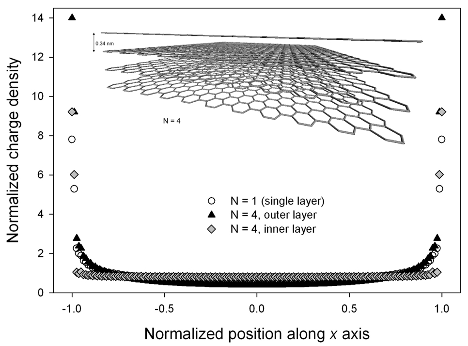
Multi-layered graphene sheets have also been studied in this work. They have been reported to have interesting electronic properties.Hass et al. (2008); Orlita et al. (2008) We investigated multi-layered graphene in which each layer contains the same quantity of net charges. Due to the electrostatic interaction between the layers, the charge profile in multi-layered graphene cannot be assumed to be a simple addition of that of a single layer. In Fig. 7, we plot the profile of net charges in a 4-layered graphene to compare with that in a single-layered one with the same size. It can be seen that the charge enhancement is more significant in multi-layered graphene. The mechanism of this behavior relies on the electrostatic repulsive effects between the carbon layers, which can effectively reduce the capacitance of the atoms at the center of graphene and can however enhance that of the edge atoms.Zdrojek et al. (2008)
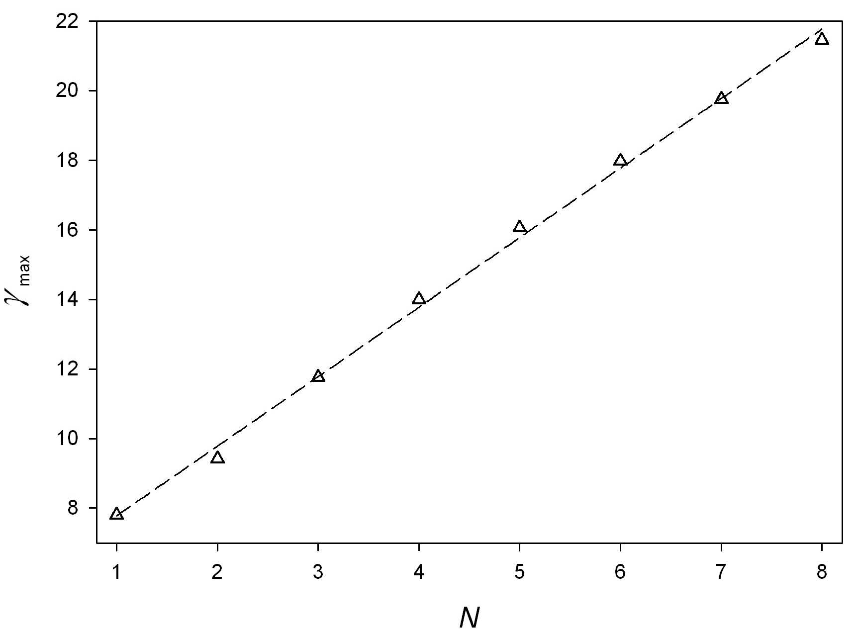
We now estimate the charge enhancement ratio in multi-layered graphene as a function of the number of layer (Fig. 8). Our results showed that the charge enhancement effect becomes more significant when the number of layer increases, due to the electrostatic repulsive effect between the layers. We found that roughly follows a linear relationship with . Note that the interlayer distance can be slightly changed in case of a very high charge density,Li and Chou (2007) while we use a constant distance nm in this work.Kolmogorov and Crespi (2000)
IV Conclusions
In conclusion, we have studied the charge distribution in graphene, using both a numerical method and an analytical solution to the classical problem of net charges in a rectangular conducting plate in three physical dimensions. It is found that the analytical model gives a good description to the charge distribution, except for the very edge atoms because of the atomic edge state. We demonstrated how the charge distribution changes with the increasing graphene length, width and number of layer. The length dependence of the charge enhancement effect was found to be related to the rise of graphene capacitance with increasing size. The charge enhancement ratio is found to follow a linear relationship with the number of layers in multi-layered graphene. These results developed a better understanding of the state of net charge in graphene, which can be useful for the potential applications of graphene in charge storages, sensors or field-emission devices.
Acknowledgements.
We gratefully thank R. Langlet and H.B. Wilson for help with the numerics. A. Mayer, M. Zdrojek, T. Melin, M. Devel and W. Ren are acknowledged for fruitful discussions.Appendix: Variational approximation for the charged rectangular plate
The desired slotion to Laplace’s equation Eq. (3) subject to the symmetric boundary conditions Eq. (4) is even in and in (and in ), so Fourier cosine integrals
| (12) |
are appropriate with . The non-analytic modulus accommodates the discontinuity in normal () derivative
| (13) |
across the surface charge. For and real, choose . Using Eq. (5), Fourier inversion of Eq. (13) is
| (14) |
The required integral is a Bessel function
| (15) |
Hence the spectral function can be expressed as
| (16) |
whereupon the forced boundary condition in Eq. (4) becomes
| (17) |
Application of the Galerkin inner-product operator
| (18) |
to each side produces
| (19) |
where and . With , we require the double integral
| (20) |
Note that . Using formulae from Watson’s treatiseWatson (1944), the square of the Bessel function is expressed as a double integral
| (21) |
of trigonometric functions, so that Eq. (20) temporarily balloons out into the six-fold integral
| (22) |
Formula 3.754(2) from Gradshteyn and RyzhikGradshteyn and Ryzhik (1994) reveals that the –integral is a modified Bessel function
| (23) |
and then their formula 6.671(14) eliminates the Bessel function in the –integral
| (24) |
Finally, the original double integral Eq. (20) of oscillatory functions over infinite ranges is converted to a four-fold integral
| (25) |
of slowly-varying functions over finite ranges. A specially designed Gaussian quadrature routine gives numerical values with little fuss. Any one of the four integrals is a complete elliptic integral, but a vectorized four-dimensional quadrature is competitive in execution time and accuracy with a thee-dimensional quadrature that requires evaluation of the elliptic function. The desired constant in Eq. (19) now takes the form in Eq. (6).
References
- Castro Neto et al. (2009) A.H. Castro Neto, F. Guinea, N.M.R. Peres, K.S. Novoselov, and A.K. Geim, Rev. Mod. Phys. 81, 109 (2009).
- Beenakker (2008) C.W.J. Beenakker, Rev. Mod. Phys. 80, 1337 (2008).
- Hwang et al. (2007) E.H. Hwang, S. Adam, and S. DasSarma, Phys. Rev. Lett. 98, 186806 (2007).
- Morozov et al. (2008) S.V. Morozov, K.S. Novoselov, M.I. Katsnelson, F. Schedin, D.C. Elias, J.A. Jaszczak, and A.K. Geim, Phys. Rev. Lett. 100, 016602 (2008).
- Fogler et al. (2008) M.M. Fogler, F. Guinea, and M.I. Katsnelson, Phys. Rev. Lett. 101, 226804 (2008).
- Son et al. (2006) Y.W. Son, M.L. Cohen, and S.G. Louie, Phys. Rev. Lett. 97, 216803 (2006).
- Yang et al. (2007) L. Yang, C.H. Park, Y.W. Son, M.L. Cohen, and S.G. Louie, Phys. Rev. Lett. 99, 186801 (2007).
- Han et al. (2007) M.Y. Han, B. Ozyilmaz, Y. Zhang, and P. Kim, Phys. Rev. Lett. 98, 206805 (2007).
- Castro et al. (2007) E.V. Castro, K.S. Novoselov, S.V. Morozov, N.M.R. Peres, J.M.B.Lopes dosSantos, Johan Nilsson, F. Guinea, A.K. Geim, and A.H. Castro Neto, Phys. Rev. Lett. 99, 216802 (2007).
- Novikov (2007) D.S. Novikov, Phys. Rev. Lett. 99, 056802 (2007).
- Yan et al. (2007) J. Yan, Y. Zhang, P. Kim, and A. Pinczuk, Phys. Rev. Lett. 98, 166802 (2007).
- Duplock et al. (2004) E.J. Duplock, M. Scheffler, and P.J.D. Lindan, Phys. Rev. Lett. 92, 225502 (2004).
- Biel et al. (2009) B. Biel, X. Blase, F. Triozon, and S. Roche, Phys. Rev. Lett. 102, 096803 (2009).
- Westervelt (2008) R.M. Westervelt, Science 320, 324 (2008).
- Paillet et al. (2005) M. Paillet, P. Poncharal, and A. Zahab, Phys. Rev. Lett. 94, 186801 (2005).
- Zdrojek et al. (2005) M. Zdrojek, T. Melin, C. Boyaval, D. Stivenard, B. Jouault, M. Wozniak, A. Huczko, W. Gebicki, and L. Adamowicz, Appl. Phys. Lett. 86, 213114 (2005).
- Jespersen and Nygard (2005) T.S. Jespersen and J. Nygard, Nano Lett. 5, 1838 (2005).
- Charlier et al. (2007) J.C. Charlier, X. Blase, and S. Roche, Rev. Mod. Phys. 79, 677 (2007).
- Morozov et al. (2006) S.V. Morozov, K.S. Novoselov, M.I. Katsnelson, F. Schedin, L.A. Ponomarenko, D. Jiang, and A.K. Geim, Phys. Rev. Lett. 97, 016801 (2006).
- Yan and Ting (2008) X.Z. Yan and C.S. Ting, Phys. Rev. Lett. 101, 126801 (2008).
- Rossi and Das Sarma (2008) E. Rossi and S. Das Sarma, Phys. Rev. Lett. 101, 166803 (2008).
- Cui et al. (2002) J.B. Cui, R. Sordan, M. Burghard, and K. Kern, Appl. Phys. Lett. 81, 3260 (2002).
- Robinson et al. (2008) J.T. Robinson, F.K. Perkins, E.S. Snow, Z. Wei, and P.E. Sheehan, Nano Lett. 8, 3137 (2008).
- Bonard et al. (2002) J.M. Bonard, K.A. Dean, B.F. Coll, and C. Klinke, Phys. Rev. Lett. 89, 197602 (2002).
- Purcell et al. (2002b) S.T. Purcell, P. Vincent, C. Journet, and V. ThienBinh, Phys. Rev. Lett. 88, 105502 (2002b).
- Maxwell (1873) J. C. Maxwell, A Treatise on Electricity and Magnetism (Clarendon Press (1891), 1873).
- Jackson (1975) J. D. Jackson, Classical Electrodynamics (Wiley, New York, 1975), p. 57-94.
- Morse and Feshbach (1953) P. M. Morse and H. Feshbach, Methods of Theoretical Physics: II (McGraw-Hill (New York), 1953), p. 1196-1197.
- Bottcher (1952) C.J.F. Bottcher, Theory of electric polarization (Elsevier (Amsterdam), 1952), p. 48-60.
- Mayer (2007) A. Mayer, Phys. Rev. B 75, 045407 (2007).
- Wang (2009) Z. Wang, Phys. Rev. B 79, 155407 (2009).
- Applequist et al. (1972) J. Applequist, J.R. Carl, and K.K. Fung, J. Am. Chem. Soc. 94, 2952 (1972).
- Olson and Sundberg (1978) M.L. Olson and K.R. Sundberg, J. Chem. Phys. 69, 5400 (1978).
- Jensen, L. (2002) L. Jensen, P.O. Astrand, A. Osted, J. Kongsted and K.V. Mikkelsen, J. Chem. Phys. 116, 4001 (2002).
- Mayer (2005a) A. Mayer, Phys. Rev. B 71, 235333 (2005a).
- Mayer (2005b) A. Mayer, Appl. Phys. Lett. 86, 153110 (2005b).
- Wang et al. (2008) Z. Wang, M. Zdrojek, T. Mélin, and M. Devel, Phys. Rev. B 78, 085425 (2008).
- Stuart et al. (2000) S.J. Stuart, A.B. Tutein, and J.A. Harrison, J. Chem. Phys. 112, 6472 (2000).
- Ni et al. (2002) B. Ni, S.B. Sinnott, P.T. Mikulski, and J.A. Harrison, Phys. Rev. Lett. 88, 205505 (2002).
- Shenoy et al. (2008) V.B. Shenoy, C.D. Reddy, A. Ramasubramaniam, and Y.W. Zhang, Phys. Rev. Lett. 101, 245501 (2008).
- (41) Z. Wang and L. Philippe, Phys. Rev. Lett. 102, 215501 (2009).
- Wang and Devel (2007) Z. Wang and M. Devel, Phys. Rev. B 76, 195434 (2007).
- Wang et al. (2007) Z. Wang, M. Devel, R. Langlet, and B. Dulmet, Phys. Rev. B 75, 205414 (2007).
- Gotoi (1992) E. Gotoi, J. Comp. Phys. 100, 105 (1992).
- Keblinski et al. (2002) P. Keblinski, S.K. Nayak, P. Zapol, and P.M. Ajayan, Phys. Rev. Lett. 89, 255503 (2002).
- Bonard et al. (1998) J.M. Bonard, T. Stockli, F. Maier, W.A. de Heer, A. Chatelain, J.P. Salvetat, and L. Forro, Phys. Rev. Lett. 81, 1441 (1998).
- Liu et al. (2009) Z. Liu, K. Suenaga, P.J.F. Harris, and S. Iijima, Phys. Rev. Lett. 102, 015501 (2009).
- Yang et al. (2008) L. Yang, M.L. Cohen, and S.G. Louie, Phys. Rev. Lett. 101, 186401 (2008).
- Abanin et al. (2006) D.A. Abanin, P.A. Lee, and L.S. Levitov, Phys. Rev. Lett. 96, 176803 (2006).
- Hass et al. (2008) J. Hass, F. Varchon, J.E. Millan-Otoya, M. Sprinkle, N. Sharma, W.A. de Heer, C. Berger, P.N. First, L. Magaud, and E.H. Conrad, Phys. Rev. Lett. 100, 125504 (2008).
- Orlita et al. (2008) M. Orlita, C. Faugeras, P. Plochocka, P. Neugebauer, G. Martinez, D.K. Maude, A.L. Barra, M. Sprinkle, C. Berger, W.A. de Heer, and M. Potemski, Phys. Rev. Lett. 101, 267601 (2008).
- Zdrojek et al. (2008) M. Zdrojek, T. Heim, D. Brunel, A. Mayer, and T. Mélin, Phys. Rev. B 77, 033404 (2008).
- Li and Chou (2007) C. Li and T.W. Chou, Carbon 45, 922 (2007).
- Kolmogorov and Crespi (2000) A.N. Kolmogorov and V.H. Crespi, Phys. Rev. Lett. 85, 4727 (2000).
- Watson (1944) G.N. Watson, A Treatise on the Theory of Bessel Functions (Cambridge University Press, 2nd Edition, 1944), p. 48, p. 151.
- Gradshteyn and Ryzhik (1994) I.S. Gradshteyn and I.M. Ryzhik, Table of Integrals, Series, and Products (Academic Press (Boston), 5th Edition, 1994).
- HarringtonMM (2009) R.F. Harrington, Field Computation by Moment Methods (Macmillan (New York), 1968), p. 24-28.
Figures