Infinite family of elliptic curves of rank at least 4

Bartosz NaskrΔ™cki Graduate School, Department of Mathematics and Computer Science, Adam Mickiewicz University, PoznaΕ„, Poland nasqret@gmail.com
Abstract.

We investigate $\mathbb{Q}$-ranks of the elliptic curve $E_{t}$: $y^{2}+txy=x^{3}+tx^{2}-x+1$ where $t$ is a rational parameter. We prove that for infinitely many values of $t$ the rank of $E_{t}(\mathbb{Q})$ is at least 4.

2000 Mathematics Subject Classification:
11D25 11G05

1. Introduction

It is of fundamental interest to find families of elliptic curves parametrized by a rational parameter with ranks higher than a prescribed constant cf. [3]. In this paper we investigate the family of curves:

(1.1) $$E_{t}:y^{2}+txy=x^{3}+tx^{2}-x+1$$

with parameter $t\in\mathbb{Q}$. We prove the following

Theorem 1.1.

For infinitely many $u\in\mathbb{Q}$ the elliptic curve over $\mathbb{Q}$ given by the affine equation $E_{(u^{2}-u-3)}:y^{2}+(u^{2}-u-3)xy=x^{3}+(u^{2}-u-3)x^{2}-x+1$ has the Mordell-Weil group of rank at least 4. More precisely, the group $E_{(u^{2}-u-3)}(\mathbb{Q})$ contains the subgroup spanned by the following linearly independent points:

$$(0,1),(1,1),(u,u+1),\left(\frac{1}{9},\frac{1}{54}(9+3u-3u^{2}+v)\right)$$

where the point $(u,v)$ lies on the elliptic curve given by the equation:

$$2569+18u-9u^{2}-18u^{3}+9u^{4}=v^{2}.$$

The latter curve has the Weierstrass model:

(1.2) $$y_{0}^{2}=x_{0}^{3}-92835x_{0}+1389150$$

which defines elliptic curve over $\mathbb{Q}$ with the Mordell-Weil group of rank 2, spanned by the points:

$$(-309,756),(-45,2340),(15,0)$$

We have checked that the curves $E_{(u^{2}-u-3)}$ have different j-invariant for all but finitely many $u\in\mathbb{Q}$ as in the statement of the theorem.

In [1] Brown and Myers constructed an infinite family of elliptic curves over $\mathbb{Q}$ with quadratic growth of parameter and the rank of the Mordell-Weil group at least 3. They proved the linear independence of classes in $E(\mathbb{Q})/2E(\mathbb{Q})$ for curves $E$ with trivial torsion. We investigate the question posed at the end of the paper [1] to find families of elliptic curves with the rank of the Mordell-Weil group higher than 3.

With the family defined in Theorem 1.1 we obtained rank 4 at cost of using Mordell’s Conjecture,i.e. theorem of Faltings. In [2] Rubin and Silverberg also obtained an infinite family of twists of elliptic curves over $\mathbb{Q}$ of rank 4. The method of [2] relies on Silverman’s specialization theorem cf. [5]. The investigated curves are in Legendre’s form. The families are parametrized by projective line or by elliptic curve of rank 1. The twists are parametrized by another elliptic curve of rank 1.

In Theorem 1.1 the parametrization of the family is given by the elliptic curve of rank 2 and we use a single parameter instead of two. Our methods are more elementary and in some places more explicit, since we don’t use specialization theorems and the coefficients of the family are at most quadratic.

Remark 1.2.

We can extend the result stated in Theorem 1.1 following [4]. Let Λ​(E/β„š,s)Ξ›πΈβ„šπ‘ \Lambda(E/\mathbb{Q},s) be the complete L-series of the elliptic curve over $\mathbb{Q}$. Denote by $W(E)\in\{\pm 1\}$ the root number in the functional equation:

(1.3) Λ​(E,2βˆ’s)=W​(E)​Λ​(E,s)Λ𝐸2π‘ π‘ŠπΈΞ›πΈπ‘ \Lambda(E,2-s)=W(E)\Lambda(E,s)

The Parity Conjecture predicts that:

(1.4) $$(-1)^{\textrm{rank}E(\mathbb{Q})}=W(E)$$

In our particular case we can compute the root number $W(E_{u})$ for the specific curves $E_{u}$ and determine the parity of the rank of group $E_{u}(\mathbb{Q})$. Since the computations can be done explicitly using primes of bad reduction of $E_{u}$ (for example using SAGE) we state the numerical results in Section 4. Assuming Parity Conjecture we construct several elliptic curves over $\mathbb{Q}$ that have rank at least 5 (Table 5).

2. Description of the algorithm

There are two obvious points lying on the curve (1.1), namely:

$$(0,1),(1,1)\in E_{u}(\mathbb{Q}(u))$$

We produce with several points with coordinates in the ring $\mathbb{Z}[u]$:

$\displaystyle-(0,1)$ $\displaystyle=$ $\displaystyle(0,-1)$
$\displaystyle-(1,1)$ $\displaystyle=$ $\displaystyle(1,-u-1)$
$\displaystyle(0,1)+2(1,1)$ $\displaystyle=$ $\displaystyle(-u+1,-1)$
$\displaystyle(0,1)+(1,1)$ $\displaystyle=$ $\displaystyle(-u-1,u^{2}+u-1)$
$\displaystyle(0,1)-(1,1)$ $\displaystyle=$ $\displaystyle(u+3,2u+5)$
$\displaystyle-(0,1)+(1,1)$ $\displaystyle=$ $\displaystyle(u+3,-u^{2}-5u-5)$
$\displaystyle-(0,1)+2(1,1)$ $\displaystyle=$ $\displaystyle(u+5,2u+11)$
$\displaystyle 2(1,1)$ $\displaystyle=$ $\displaystyle(-1,u+1)$

In order to find more points on the curve (1.1) we specialize parameter $u$ to a polynomial function of another parameter $v\in\mathbb{Q}$:

$$u(v)=a_{n}v^{n}+\ldots+a_{1}v+a_{0}$$

where $a_{i}\in\mathbb{Q}$. To get a rational point on the curve (1.1) with x-coordinate $av+b$ and $a,b\in\mathbb{Q}$ it is necessary and sufficient:

(2.1) $$\Delta(v)=4(-1+b+av)^{2}(1+b+av)+(2+u(v))^{2}(b+av)^{2}$$

is a perfect square.

Lemma 2.1.

Let $P=(x,y)$ be a rational point on the curve $E_{u}(v)$ over $\mathbb{Q}(v)$ where $u(v)=a_{n}v^{n}+\ldots+a_{1}v+a_{0}\in\mathbb{Q}[v]$ of positive degree. Let $x=av+b\in\mathbb{Q}[v]$. Since aβ‰ 0π‘Ž0a\neq 0 it follows that:

  1. (i)

    $deg(u)=1\Longrightarrow$ $P=k(0,1)+l(1,1)$ for some $k,l\in\mathbb{Z}$

  2. (ii)

    $deg(u)=2\Longrightarrow$ $P=(x,x+1)$ and $u=x^{2}-x-3$ or $P=(x,x-1)$ and $u=-x^{2}+x+1$

  3. (iii)

    For any $u(v)$ with $deg(u)>2$ there is no rational point with x-coordinate equal to $av+b\in\mathbb{Q}[v]$ with aβ‰ 0π‘Ž0a\neq 0.

Proof.

Assume $u=u(v)=a_{1}v+a_{0}$ and a1,aβ‰ 0subscriptπ‘Ž1π‘Ž0a_{1},a\neq 0. Put $\Delta(v)=(q_{2}v^{2}+q_{1}v+q_{0})^{2}$ and comparing coefficients of (2.1) and $P(v)$ in descending order we find:

$$q_{2}=\epsilon aa_{1}$$
$$q_{1}=\frac{2a^{2}+2aa_{1}+aa_{0}a_{1}+ba_{1}^{2}}{\epsilon a_{1}}$$
$$q_{0}=\frac{-2a^{3}-4a^{2}a_{1}-2a^{2}a_{0}a_{1}-2aa_{1}^{2}+4aba_{1}^{2}+2ba_{1}^{3}+ba_{0}a_{1}^{3}}{\epsilon a_{1}^{3}}$$

for $\epsilon=\pm 1$. Equating the last two coefficients gives two equations in variables $a_{1},a_{0},a,b$:

$\displaystyle R_{1}(a,b,a_{0},a_{1})=-a^{6}-4a^{5}a_{1}-2a^{5}a_{0}a_{1}-6a^{4}a_{1}^{2}+4a^{4}ba_{1}^{2}-4a^{4}a_{0}a_{1}^{2}$
$\displaystyle-a^{4}a_{0}^{2}a_{1}^{2}-4a^{3}a_{1}^{3}+10a^{3}ba_{1}^{3}-2a^{3}a_{0}a_{1}^{3}+5a^{3}ba_{0}a_{1}^{3}-a^{2}a_{1}^{4}$
$\displaystyle+8a^{2}ba_{1}^{4}-4a^{2}b^{2}a_{1}^{4}+4a^{2}ba_{0}a_{1}^{4}+a^{2}ba_{0}^{2}a_{1}^{4}$
$\displaystyle+2aba_{1}^{5}-4ab^{2}a_{1}^{5}+aba_{0}a_{1}^{5}-2ab^{2}a_{0}a_{1}^{5}+a_{1}^{6}-ba_{1}^{6}-b^{2}a_{1}^{6}+b^{3}a_{1}^{6}=0$
$\displaystyle R_{2}(a,b,a_{0},a_{1})=2a^{4}+6a^{3}a_{1}+3a^{3}a_{0}a_{1}+6a^{2}a_{1}^{2}-3a^{2}ba_{1}^{2}+4a^{2}a_{0}a_{1}^{2}$
$\displaystyle+a^{2}a_{0}^{2}a_{1}^{2}+2aa_{1}^{3}-4aba_{1}^{3}+aa_{0}a_{1}^{3}-2aba_{0}a_{1}^{3}-a_{1}^{4}-ba_{1}^{4}+b^{2}a_{1}^{4}=0$

The ideal $I=I(R_{1},R_{2})$ of the equations can be rearranged to the form of the GrΓΆbner basis $I=I(a^{9}-2a^{7}a_{1}^{2}+a^{5}a_{1}^{4},R^{\prime}_{1},\ldots,R^{\prime}_{18})$ with $R^{\prime}_{i}=R^{\prime}_{i}(a,b,a_{0},a_{1})$. It implies $a=\pm a_{1}$. For $a=a_{1}$ the equations reduce to:

$$a_{0}=-3+b$$

or

$$a_{0}=-5+b.$$

For $t=av+b-3$ or $t=av+b-5$ we get points $(t+3,5+2t),(t+3,-5-5t-t^{2})$ and $(t+5,11+2t),(t+5,-11-7t-t^{2})$ respectively. If $u=t$ all these points are linear combinations of $(0,1)$ and $(1,1)$ as on the list above. For $a=-a_{1}$ the equations reduce to:

$$a_{0}=-1-b$$

or

$$a_{0}=1-b.$$

For $t=-av-b-1$ or $t=-av-b+1$ we get points $(-t-1,1),(-t-1,-1+t+t^{2})$ and $(-t+1,-1),(-t+1,1-t+t^{2})$ respectively. Again for $u=t$ all points are the linear combinations of $(0,1)$ and $(1,1)$.

Assume $u=u(v)=a_{2}v^{2}+a_{1}v+a_{0}$ and a1,aβ‰ 0subscriptπ‘Ž1π‘Ž0a_{1},a\neq 0. Put $P(v)=(q_{3}v^{3}+q_{2}v^{2}+q_{1}v+q_{0})^{2}$. Comparing coefficients of (2.1) and $P(v)$ implies:

$$q_{3}=\epsilon aa_{2}$$
$$q_{2}=\frac{aa_{1}+ba_{2}}{\epsilon}$$
$$q_{1}=\frac{2a+aa_{0}+ba_{1}}{\epsilon}$$
$$q_{0}=\frac{2a^{2}+2ba_{2}+ba_{0}a_{2}}{\epsilon a_{2}}$$

with $\epsilon=\pm 1$. This gives:

$$a_{1}=\frac{(-1+2b)a_{2}}{a}$$
$$a^{3}\left(2+a_{0}\right)+a\left(1+b-b^{2}\right)a_{2}=0$$
$$a^{2}=\lambda a_{2}$$

with $\lambda=\pm 1$. It implies $u(v)=-2-\lambda-t\lambda+t^{2}\lambda$, where $t=av+b$. In this way we get two distinct families:

Table 1. Families
Point Parameter u
Family A $(t,t+1)$ $t^{2}-t-3$
Family B $(t,t-1)$ $-t^{2}+t+1$

Consider $u(v)$ as a polynomial in $v$ of degree $n>2$ then $deg(\Delta)=2n+2$ so we look for the polynomial $P(v)$ of degree $n+1$. We put:

$$a^{*}_{i}=a_{i}$$
$$q^{*}_{j}=q_{j}$$

for $0<i\leq n$ and $0\leq j\leq n+1$,$a^{*}_{0}=a_{0}+2$. For other $i,j$ put:

$$a^{*}_{i}=0$$
$$q^{*}_{j}=0$$

We prove by induction the following formula:

$$q^{*}_{j}=\epsilon(aa^{*}_{j-1}+bb^{*}_{j})$$

using the identities:

$$c_{j}(\Delta)=a^{2}\sum_{j=\alpha+\beta}a^{*}_{\alpha}a^{*}_{\beta}+2ab\sum_{j+1=\alpha+\beta}a^{*}_{\alpha}a^{*}_{\beta}+b^{2}\sum_{j+2=\alpha+\beta}a^{*}_{\alpha}a^{*}_{\beta}$$
$$c_{j}(P^{2})=\sum_{j=\alpha+\beta}q^{*}_{\alpha}q^{*}_{\beta}$$

for $j=n+1,...,2n+2$, where $c_{j}(a_{0}+a_{1}x+\ldots+a_{n}x^{n})=a_{j}$.It follows from $\Delta=P^{2}$:

$$c_{j}(\Delta)=c_{j}(P^{2}).$$

We substitute the coefficients $q_{0}=\epsilon(2b+ba_{0})$ and $q_{1}=\epsilon(a(a_{0}+2)+ba_{1})$ into the identities above with $j=0,1,2$ and we get $b^{2}=1$ and finally $a=0$, a contradiction. This completes the proof of the lemma. ∎

By Lemma 2.1, we can specialize to one of the quadratic parameters, since the families given by Table 1 have similar properties. By abuse of notation, we use the same letter $u^{2}-u-3$ for the parameter u. From now on the curve $E_{u}$ will be defined by the equation:

$$y^{2}+(u^{2}-u-3)xy=x^{3}+(u^{2}-u-3)x^{2}-x+1.$$

For simplicity of notation, we write $f(x,y,u)=0$ instead of the equation above. The point $(u,u+1)$ lies on these curves and gives several new integral points over $\mathbb{Q}[u]$:

$\displaystyle-(u,u+1)$ $\displaystyle=$ $\displaystyle(u,-u^{3}+u^{2}+2u-1)$
$\displaystyle(0,1)+(u,u+1)$ $\displaystyle=$ $\displaystyle(-u+1,u^{3}-2u^{2}-u+1)$
$\displaystyle(1,1)-(u,u+1)$ $\displaystyle=$ $\displaystyle(u^{3}-2u,u^{4}+u^{3}-3u^{2}-2u+1)$
$\displaystyle 2(1,1)+(u,u+1)$ $\displaystyle=$ $\displaystyle(-u^{3}+4u^{2}-6u+4,u^{5}-6u^{4}+14u^{3}-17u^{2}+10u-1)$

In order to find the fourth linearly independent rational point on the curve $E_{u}$ we consider the following general algorithm:

  1. (1)

    Choose two rational functions $a(x),b(x)\in\mathbb{Q}(x)$.

  2. (2)

    Set the simultaneous equations of the form:

    $\displaystyle f(a(u),y_{a}(u),u)$ $\displaystyle=$ $\displaystyle 0$
    $\displaystyle f(b(u),y_{b}(u),u)$ $\displaystyle=$ $\displaystyle 0$
  3. (3)

    Find such $a(x),b(x)$ that $y_{a}(x),y_{b}(x)\in\mathbb{Q}(x)$.

  4. (4)

    Sufficient and necessary condition for $y_{a},y_{b}$ to be rational is that the discriminant of the quadratic equation $f(a(x),y_{a},x)=0$ in $y_{a}$ is a perfect square. The same condition holds for the equation in $y_{b}$.

  5. (5)

    Find all rational points (the triples $(u,s,t)\in\mathbb{Q}^{3}$ on the affine curve):

    (2.2) $\displaystyle\Delta_{f(a(x),y_{a},x)=0}(u)$ $\displaystyle=$ $\displaystyle s^{2}$
    $\displaystyle\Delta_{f(b(x),y_{b},x)=0}(u)$ $\displaystyle=$ $\displaystyle t^{2}$

    where $\Delta_{f(a(x),y_{a},x)=0}(x),\Delta_{f(b(x),y_{b},x)=0}(x)\in\mathbb{Q}[x]$

We pick now $a(x)=x$ and $b(x)=c$. The first equation (2.2) reduces to:

$$(2-u-u^{2}+u^{3})^{2}=s^{2}$$

while the second gives:

$$4-4c-3c^{2}+4c^{3}+2c^{2}u-c^{2}u^{2}-2c^{2}u^{3}+c^{2}u^{4}=t^{2}.$$

We choose such a $c\in\mathbb{Q}$ that it defines the elliptic curve in quartic form with infinitely many points $(u,t)$. Direct search with $u\in\mathbb{N}$ reveals that for $u=7$ we have on the curve $E_{7}$ four linearly independent points:

$$(0,1),(1,1),(7,8),(\frac{1}{9},\frac{8}{27})$$

though we put $c=\frac{1}{9}$(as in the statement of Theorem 1.1).

3. Proofs

In order to prove Theorem 1.1 we will need the following elementary lemma:

Lemma 3.1.

Let M be a left $\mathbb{Z}-module$. Given any $b\in M$ suppose that $a_{1},\ldots,a_{k}\in M$ are linearly independent over $\mathbb{Z}$ and the nonzero cosets $[a_{1}],\ldots,[a_{k}]\in M/2M$ are linearly independent over $\mathbb{F}_{2}$. If $[b]\notin\langle[a_{1}],\ldots,[a_{k}]\rangle$ and $M[2]={0}$, two-torsion of M is trivial, then $b,a_{1},\ldots,a_{k}$ are independent over $\mathbb{Z}$ in M.

Proof.

Suppose, contrary to our claim, that there exists $\alpha_{1},\ldots,\alpha_{k},\beta\in\mathbb{Z}$,not all zero, such that:

$$\beta b+\alpha_{1}a_{1}+\ldots+\alpha_{k}a_{k}=0.$$

We can assume that $\beta$ is the least positive integer for which the last equation holds. If $\beta$ is odd:

$$[\beta b]=[b]$$

and

$$[b]=[\alpha_{1}a_{1}+\ldots+\alpha_{k}a_{k}]$$

which is a contradiction. If $\beta$ is even:

$$[0]=[\alpha_{1}a_{1}+\ldots+\alpha_{k}a_{k}]$$

The linear independence of cosets $[a_{i}]$ over $\mathbb{F}_{2}$ implies that all $\alpha_{i}$ are even. So it is possible to write:

$$\beta^{\prime}b=\alpha_{1}^{\prime}a_{1}+\ldots+\alpha_{k}^{\prime}a_{k}$$

where $2\beta^{\prime}=\beta$ and $2\alpha_{i}^{\prime}=\alpha_{i}$. Again the contradiction with the minimality of $\beta$. ∎

Let $M=E_{u}(\mathbb{Q})$. First we compute the rational 2-torsion for the curve $E_{u}$. For a point $P=(x,y)$ on the curve $y^{2}+(u^{2}-u-3)xy=x^{3}+(u^{2}-u-3)x^{2}-x+1$ the negative is equal:

$$-P=(x,(-u^{2}+u+3)x-y)$$

We find the following condition for the point to be a 2-torsion point:

$$1-x+\frac{1}{4}(4(-3-u+u^{2})+(-3-u+u^{2})^{2})x^{2}+x^{3}=0$$

Computing with Maple we find that the equation defines a hyperelliptic curve of genus 2. With substitutions:

(3.1) $\displaystyle x_{0}$ $\displaystyle=\frac{-1-ux+xu^{2}}{x-1}$
(3.2) $\displaystyle y_{0}$ $\displaystyle=-4x+8ux$

the curve transforms birationally into the form:

(3.3) $$y_{0}^{2}=-55+192x_{0}-114x_{0}^{2}+68x_{0}^{3}-15x_{0}^{4}+4x_{0}^{5}.$$
Lemma 3.2.

For all but finitely many $u\in\mathbb{Q}$ the rational 2-torsion of elliptic curve $E_{u}$ over $\mathbb{Q}$ is trivial.

Proof.

This is an immediate corollary of the above calculation and Mordell’s conjecture proven by Faltings, since the curve (3.3) has nonsingular model and the genus is 2. ∎

Proof of Theorem 1.1.

In order to prove Theorem 1.1 we check if the apropriate points and their linear combinations belong to $2E_{u}(\mathbb{Q})$. Given a $\mathbb{Q}$-rational point $P=(x,y)$ on the curve $E_{u}$ over $\mathbb{Q}$ we have the following formula for the x-coordinate of the point $2P$:

$$x(2P)=\frac{4-2u+u^{2}+2u^{3}-u^{4}-8x+2x^{2}+x^{4}}{4-4x+(-3+2u-u^{2}-2u^{3}+u^{4})x^{2}+4x^{3}}.$$

To ease notation define:

$$P_{\varepsilon_{1},\varepsilon_{2},\varepsilon_{3}}=\varepsilon_{1}(0,1)+\varepsilon_{2}(1,1)+\varepsilon_{3}(u,u+1)$$

If for $u\in\mathbb{Q}$ there exists a rational point $(\frac{1}{9},y)$ on the curve $E_{u}$ and $y$ is one of two values:

$$y=\frac{1}{54}(9+3u-3u^{2}\pm\sqrt{2569+18u-9u^{2}-18u^{3}+9u^{4}})$$

then we put:

$$Q_{\varepsilon_{1},\varepsilon_{2},\varepsilon_{3},\varepsilon_{4}}=\varepsilon_{1}(0,1)+\varepsilon_{2}(1,1)+\varepsilon_{3}(u,u+1)+\varepsilon_{4}(1/9,y)$$

where $\varepsilon_{i}\in\{-1,0,1\}$. The proof separates naturally into two distinct parts. In the first part we establish the criteria for which the equations:

$$P_{\varepsilon_{1},\varepsilon_{2},\varepsilon_{3}}=x(2P)$$

and

$$Q_{\varepsilon_{1},\varepsilon_{2},\varepsilon_{3},\varepsilon_{4}}=x(2P)$$

have solutions in pairs of rational numbers $(u,x)$ (recall that $P=(x,y)$ lies on $E_{u}$). In the second part of the proof we gather information to find the infinite subset of $\mathbb{Q}$ of parameters $u$ for which the rank is at least 4. To use Lemma 3.1 we must consider the tuples:

(3.4) $$(\varepsilon_{1},\varepsilon_{2},\varepsilon_{3})\in\{(1,0,0),(0,1,0),(0,0,1),(1,1,0),(0,1,-1),(1,0,1),(1,1,1)\}$$

Assume that $(\frac{1}{9},y)$ is $\mathbb{Q}$-rational. We consider:

(3.5) $$(\varepsilon_{1},\varepsilon_{2},\varepsilon_{3},\varepsilon_{4})\in\{(0,0,0,1),(1,0,0,1),(0,1,0,1),\\ (0,0,1,1),(1,1,0,1),(0,1,-1,1),(1,0,1,1),(1,1,1,1)\}$$

The tuples with negative entries were chosen to lower the genera of corresponding curves. Since we work mod $2E(\mathbb{Q})$ the tuples can be chosen quite arbitrarily. We compute genera of curves using genus command from algcurves package in Maple 12. We consider the following separate cases:

Case I: $(\varepsilon_{1},\varepsilon_{2},\varepsilon_{3})=(1,0,0)$
The tuple implies the following equation:

(3.6) $$\frac{4-2u+u^{2}+2u^{3}-u^{4}-8x+2x^{2}+x^{4}}{4-4x+(-3+2u-u^{2}-2u^{3}+u^{4})x^{2}+4x^{3}}=0$$

Since (0,1)β‰ π’ͺ01π’ͺ(0,1)\neq\mathcal{O}, the point at infinity, then the denominator is nonvanishing and:

$$4-2u+u^{2}+2u^{3}-u^{4}-8x+2x^{2}+x^{4}=0$$

It defines an elliptic curve of rank 1. By the following formulas:

$\displaystyle x_{0}$ $\displaystyle=\frac{1}{3\left(u^{2}-u-1\right)}(12u^{4}-12u^{3}x-36u^{3}+12u^{2}x^{2}+30u^{2}x$
$\displaystyle+35u^{2}-12ux^{3}-24ux^{2}-42ux+61u+18x^{3}+6x^{2}+36x-113)$
$\displaystyle y_{0}$ $\displaystyle=-\frac{1}{u^{2}-u-1}(2(8u^{5}-8u^{4}x-32u^{4}+8u^{3}x^{2}+28u^{3}x$
$\displaystyle+44u^{3}-8u^{2}x^{3}-24u^{2}x^{2}-39u^{2}x+9u^{2}+20ux^{3}$
$\displaystyle+20ux^{2}+43ux-101u-19x^{3}-11x^{2}-54x+122))$

the equation transforms to the short Weierstrass form:

$$y_{0}^{2}=x_{0}^{3}+\frac{359}{3}x_{0}+\frac{3130}{27}.$$

The Mordell-Weil group of this elliptic curve is generated by the point $(\frac{53}{3},88)$. Hence in the original form the generator is equal to $(u,x)=(\frac{1}{2},\frac{1}{2})$. Similar calculations and computation with Maple of the genus are summarized in the table (2).

Table 2. Other curves
$(\varepsilon_{1},\varepsilon_{2},\varepsilon_{3})$ genus
$(1,0,0)$ 1
$(0,1,0)$ 3
$(0,0,1)$ 2
$(1,1,0)$ 3
$(0,1,-1)$ 4
$(1,0,1)$ 2
$(1,1,1)$ 4

Assume now that we are given a point $(\frac{1}{9},y)$ rational, lying on the curve $E_{u}$ for a suitable $u\in\mathbb{Q}$.

Case II: $(\varepsilon_{1},\varepsilon_{2},\varepsilon_{3},\varepsilon_{4})=(0,0,0,1)$

(3.7) $$\frac{-u^{4}+2u^{3}+u^{2}-2u+x^{4}+2x^{2}-8x+4}{\left(u^{4}-2u^{3}-u^{2}+2u-3\right)x^{2}+4x^{3}-4x+4}=\frac{1}{9}$$

The equation above defines affine curve of genus 5.

Case III: $(\varepsilon_{1},\varepsilon_{2},\varepsilon_{3},\varepsilon_{4})=(1,0,0,1)$

(3.8) $$\frac{-u^{4}+2u^{3}+u^{2}-2u+x^{4}+2x^{2}-8x+4}{\left(u^{4}-2u^{3}-u^{2}+2u-3\right)x^{2}+4x^{3}-4x+4}=-9u^{2}+9u-162y+180$$

From the equation of the curve $E_{u}$ we can find the following formula:

$$y=\frac{1}{54}\left(-3u^{2}+3u+v+9\right)$$
$$v=\pm\sqrt{2569+18u-9u^{2}-18u^{3}+9u^{4}}$$

Using these relations we can assume that if a point (x,u) lies on the curve defined as in (3.8) then it also lies on the curve:

(3.9) $$9(9u^{4}-18u^{3}-9u^{2}+18u+2569)(u^{4}x^{2}-2u^{3}x^{2}-u^{2}x^{2}\\ +2ux^{2}+4x^{3}-3x^{2}-4x+4)^{2}-(153u^{4}x^{2}\\ +u^{4}-306u^{3}x^{2}-2u^{3}-153u^{2}x^{2}-u^{2}\\ +306ux^{2}+2u-x^{4}+612x^{3}-461x^{2}-604x+608)^{2}=0$$

This curve has genus 9. The rest is computed in a similar way (cf. Table 3).

Table 3. Other curves
$(\varepsilon_{1},\varepsilon_{2},\varepsilon_{3},\varepsilon_{4})$ genus
$(0,0,0,1)$ 5
$(1,0,0,1)$ 9
$(0,1,0,1)$ 13
$(0,0,1,1)$ 19
$(1,1,0,1)$ 13
$(0,1,-1,1)$ 15
$(1,0,1,1)$ 11
$(1,1,1,1)$ 28

In the last step of the proof we show for which $u\in\mathbb{Q}$ the point $(\frac{1}{9},y)$ is $\mathbb{Q}$-rational. It is straightforward to compute the root $y$:

$$-\frac{649}{729}+\frac{1}{81}\left(3+u-u^{2}\right)+\frac{1}{9}\left(-3-u+u^{2}\right)y+y^{2}=0$$
$$y=\frac{1}{54}\left(9+3u-3u^{2}\pm\sqrt{2569+18u-9u^{2}-18u^{3}+9u^{4}}\right)$$

Hence $y\in\mathbb{Q}$ if and only if $2569+18u-9u^{2}-18u^{3}+9u^{4}$ is a full square. This condition defines the elliptic curve in a quartic form. It is birational to elliptic curve in the Weierstrass form:

$$y_{0}^{2}=x_{0}^{3}-92835x_{0}+1389150.$$

The Mordell-Weil group of the curve has rank 2. The torsion subgroup is isomorphic to $\mathbb{Z}/2$. Generators of the free part are $(x_{0},y_{0})=(-309,-756),(390,-4950)$ and the generator of the torsion subgroup is $(15,0)$. In the quartic form they correspond to:

$$\left(\frac{1}{9},\frac{1369}{27}\right),\left(\frac{27}{10},\frac{-5173}{100}\right),\left(-6,-133\right)$$

respectively.

Consider the curve $y^{2}+uxy=x^{3}+ux^{2}-x+1$. The only critical value which gives an infinite subset of parameters $u\in\mathbb{Q}$ was obtained from doubling the point $(0,1)$. We consider this case if the point $(\frac{1}{9},y)$ on the curve $y^{2}+uxy=x^{3}+ux^{2}-x+1$ is $\mathbb{Q}$-rational. Solving the quadratic equation gives:

$$y=\frac{1}{54}\left(-3u\pm\sqrt{2596+36u+9u^{2}}\right).$$

The point $(0,1)$ is a double and $(\frac{1}{9},y)$ is a rational point when we have the rational point on the curve:

(3.10) $\displaystyle s^{2}$ $\displaystyle=2596+36u+9u^{2}$
(3.11) $\displaystyle 0$ $\displaystyle=1-4u-u^{2}-8x+2x^{2}+x^{4}.$

Parametrization of the first equation gives:

(3.12) $\displaystyle u$ $\displaystyle=\frac{2596-t^{2}}{6t-36}$
(3.13) $\displaystyle s$ $\displaystyle=\frac{t^{2}-12t+2596}{2t-12}$

with a new parameter $t\in\mathbb{Q}\backslash\{6\}$. Substituting into the second equation gives the curve:

(3.14) $$(-6364096-62736t+5084t^{2}+24t^{3}-t^{4}-10368x\\ +3456tx-288t^{2}x+2592x^{2}-864tx^{2}+72t^{2}x^{2}\\ +1296x^{4}-432tx^{4}+36t^{2}x^{4})$$

This curve has genus 3, so it has finitely many rational points. Specializing to a parameter $u^{2}-u-3$ we obtain that there are only finitely many $u\in\mathbb{Q}$ for which $(0,1)$ is a double while $(\frac{1}{9},y)$ is $\mathbb{Q}$-rational. From the infinite family of parameters $u$ chosen from the first coordinate of the elliptic curve over $\mathbb{Q}$:

$$2569+18u-9u^{2}-18u^{3}+9u^{4}=v^{2}$$

we have excluded only finitely many $u$ due to the doubling restrictions given in Table 2 and Table 3. It remains to show that the j-invariant of the curve $F_{u}:y^{2}+uxy=x^{3}+ux^{2}-x+1$ repeats itself for finitely many $u\in\mathbb{Q}$. We compute:

(3.15) $$j(F_{u})=-\frac{(48+u^{2}(4+u)^{2})^{3}}{(2+u)^{2}(92+(-1+u)u(4+u)(5+u))}$$

Hence the equation:

$$j(F_{u})=j(F_{v})$$

defines an affine curve with coordinates $(u,v)$ which has genus 11 according to computations in Maple. This implies that specializing the parameter $u$ to $u^{2}-u-3$ gives a curve with finitely many points. ∎

4. Numerical results

4.1. General statistics

We show the statistics of ranks for the family of curves:

$$y^{2}+uxy=x^{3}+ux^{2}-x+1$$

with parameter $u\in\mathbb{N}$. All computations were performed with SAGE 3.4 with mwrank procedure. For some points there is no proof for the upper bound of the rank (in that case the value is excluded).

Figure 1. Rank statistics
Refer to caption

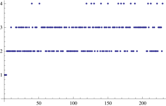
We can compute the percentage of curves of each type (Table 4).

Table 4. Curves of certain ranks
rank percentage
1 1%
2 41%
3 45%
4 7%
unproven 6%

More interesting is the plot of curves of rank 3 (Figure 2)

Figure 2. Curves of rank 3
Refer to caption

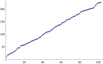
which shows that progression for curves of rank 3 is almost linear. It suggests that we can use the general algorithm from the introduction to state another version of the main theorem 1.1 and find many more infinite families of elliptic curves over $\mathbb{Q}$.

4.2. Explicit version of the main theorem

The statement of the theorem requires removing a finite subset of ’bad rational points’ due to Falting’s Theorem(Mordell’s Conjecture). The upper bound of heights of this points is hard to obtain. We shall give an explicit and effective version of the main result of this paper. However for rational points on the curve (1.2) with low height we can compute the explicit table of corresponding elliptic curves $E_{u}$ over $\mathbb{Q}$ of rank at least 4. The curve:

(4.1) $$C_{1}:y_{0}^{2}=x_{0}^{3}-92835x_{0}+1389150$$

is mapped to the curve:

(4.2) $$C_{2}:2569+18u-9u^{2}-18u^{3}+9u^{4}=v^{2}$$

via the map:

$$\phi:C_{1}\longrightarrow C_{2}$$

where $\phi(x_{0},y_{0})=(u,v)$ is given by the formulas:

$$u=\frac{565605+x_{0}(-948+7x_{0})+266y_{0}}{(-1551+x_{0})(45+x_{0})}$$
$\displaystyle v=\frac{1}{(-1551+x_{0})^{2}(45+x_{0})^{2}}\left(133(92385+(-30+x_{0})x_{0})(-115425+x_{0}(1536+x_{0}))\right.+$
$\displaystyle\left.234(-3922935+x_{0}(9010+41x_{0}))y_{0}\right)$

and defined at the points $(-45,2340)$,$(-45,-2340)$, $(1551,59904)$, $(1551,-5990)$, $\infty_{C_{1}}$:

$\displaystyle\phi(-45,2340)$ $\displaystyle=\infty_{C_{2}}$
$\displaystyle\phi(-45,-2340)$ $\displaystyle=(-\frac{10898}{5187},-\frac{477412081}{8968323})$
$\displaystyle\phi(1551,59904)$ $\displaystyle=\infty_{C_{2}}$
$\displaystyle\phi(1551,-59904)$ $\displaystyle=(\frac{16085}{5187},\frac{477412081}{8968323})$
$\displaystyle\phi(\infty_{C_{1}})$ $\displaystyle=(7,133)$

for $\infty_{C_{1}}$ - the point at infinity $C_{1}$ and analogously for $C_{2}$. The map is regular at every point of $C_{1}$ so it is a morphism of curves. For the converse we have the mapping:

$$\psi:C_{1}\longrightarrow C_{2}$$

where $\psi(u,v)=(x_{0},y_{0})$ with:

$$x_{0}=\frac{5117-948u+753u^{2}+266v}{(-7+u)^{2}}$$
$$y_{0}=\frac{266(5201+9u(-4+u(-22+13u)))+2(1799+4797u)v}{(-7+u)^{3}}$$

which is not regular at the point $\infty_{C_{2}}$ and is defined at the points $(7,133)$ and $(7,-133)$:

$\displaystyle\psi(7,133)$ $\displaystyle=\infty_{C_{1}}$
$\displaystyle\psi(7,-133)$ $\displaystyle=(-\frac{3628425}{17689},\frac{8081948160}{2352637})$

If we define sets:

$$A=C_{1}\backslash\{(-45,2340),(1551,59904)\}$$
$$B=C_{2}\backslash\{\infty_{C_{2}}\}$$

Then we have:

$$\phi\circ\psi=id_{A}$$
$$\psi\circ\phi=id_{B}$$

We now give the explicit table of curves of rank at least 4 as stated in the main theorem. If we assume the Parity Conjecture we can show that some of them have actually the rank at least 5. Let $E_{u}:y^{2}+(u^{2}-u-3)xy=x^{3}+(u^{2}-u-3)x^{2}-x+1$ and $P_{1}=(-309,756)$, $P_{2}=(-45,2340)$, $T=(15,0)$ - the points spanning the group $C_{1}(\mathbb{Q})$. From the computations above we can associate uniquely a pair $(u,v)$ on $C_{2}$ corresponding to the point $\alpha T+\beta_{1}P_{1}+\beta_{2}P_{2}$. We abbreviate this as $(u,v)\leftrightarrow(\alpha,\beta_{1},\beta_{2})$. We define the following functions:

  • β€’

    R​(u)𝑅𝑒R(u) is the regulator of points $(0,1),(1,1),(u,u+1),\left(\frac{1}{9},\frac{1}{54}(9+3u-3u^{2}+v)\right)$

  • β€’

    N​(u)𝑁𝑒N(u) is the conductor of the curve $E_{u}$

  • β€’

    j​(u)𝑗𝑒j(u) is the j-invariant of $E_{u}$

  • β€’

    W​(u)π‘Šπ‘’W(u) is equal to the global root number $W(E_{u}/\mathbb{Q})$.

All the computations were performed for the minimal model of each curve.

Table 5. Curves of rank 4 and 5

$(\alpha,\beta_{1},\beta_{2})$ R(u) N(u) j(u) W(u) Rank ( 0 , -2 , -2 ) 253637.08 $7.42\times 10^{117}$ -4382.17 -1 $\geq 5$ ( 0 , -2 , -1 ) 53400.57 $4.79\times 10^{79}$ $-1.39\times 10^{6}$ 1 $\geq 4$ ( 0 , -2 , 0 ) 16681.20 $5.69\times 10^{59}$ $-4.14\times 10^{11}$ -1 $\geq 5$ ( 0 , -2 , 1 ) 23528.39 $1.89\times 10^{64}$ $-1.11\times 10^{16}$ 1 $\geq 4$ ( 0 , -1 , -2 ) 117347.77 $1.22\times 10^{95}$ $-4.66\times 10^{19}$ 1 $\geq 4$ ( 0 , -1 , -1 ) 6398.35 $2.46\times 10^{46}$ $-7.42\times 10^{8}$ 1 $\geq 4$ ( 0 , -1 , 0 ) 28.40 $4.13\times 10^{12}$ -1255.79 1 $\geq 4$ ( 0 , -1 , 1 ) 0.0 $6.54\times 10^{11}$ -1264.95 1 - ( 0 , 0 , -2 ) 138113.04 $6.46\times 10^{98}$ -912.11 -1 $\geq 5$ ( 0 , 0 , -1 ) 4697.68 $1.21\times 10^{43}$ -20742.18 1 $\geq 4$ ( 0 , 0 , 0 ) 8.61 57482738.0 $-4.72\times 10^{9}$ 1 $\geq 4$ ( 0 , 1 , -2 ) 608830.99 $3.64\times 10^{145}$ $-4.45\times 10^{19}$ 1 $\geq 4$ ( 0 , 1 , -1 ) 56796.71 $1.80\times 10^{81}$ $-3.75\times 10^{10}$ -1 $\geq 5$ ( 0 , 1 , 0 ) 1301.45 $8.98\times 10^{31}$ -200862.89 -1 $\geq 5$ ( 0 , 1 , 1 ) 0.0 $6.54\times 10^{11}$ -1264.95 1 -

For the last tuple the regulator is equal to 0 because the tuple corresponds to $u=\frac{1}{9}$ for which the fourth point from the statement of Theorem 1.1 coincides with the third point. For the tuple $(0,-1,1)$ (when $u=8/9$) the fourth point is linearly dependent on the other three points. Moreover the curves corresponding to these tuples are isomorphic over $\mathbb{Q}$.

Remark 4.1.

We can find in the family $E_{u}$ curves of unconditional rank at least five. The curve $E_{16}:y^{2}+239xy=x^{3}+239x^{2}-x+1$ is a curve of unconditional rank five. The set of generators of the non-torsion part is given by:

$$(0,1),(1,1),(16,17),(-14/25,16661/125),(52/81,469/729)$$

We can show that for $c=-14/25$ the associated auxiliary elliptic curve from Theorem 1.1:

$$4-4c-3c^{2}+4c^{3}+2c^{2}u-c^{2}u^{2}-2c^{2}u^{3}+c^{2}u^{4}=t^{2}$$

has rank 4 over $\mathbb{Q}$. This might lead to alternative formulation of Theorem 1.1.

Acknowledgments

The author would like to thank Wojciech Gajda for suggesting the problem. He thanks Sebastian Petersen for helpful comments concerning root numbers and the Parity Conjecture. The author is grateful to Adam Lipowski for the computational resources supporting SAGE 3.4.

References

  • [1] E.Brown; B.T.Myers, Elliptic curves from Mordell to Diophantus and back., Am. Math. Mon. 109, No.7, 639-649 (2002).
  • [2] K.Rubin and A.Silverberg, Twists of elliptic curves of rank at least four. In Ranks of elliptic curves and random matrix theory, (J. B. Conrey, D. W. Farmer, F. Mezzadri and N. C. Snaith, ed.), London Mathematical Society Lecture Note Series, 341, $177-188$, Cambridge University Press, Cambridge, 2007.
  • [3] J. B. Conrey, D. W. Farmer, F. Mezzadri and N. C. Snaith, ed., Ranks of elliptic curves and random matrix theory, London Mathematical Society Lecture Note Series, 341, $177-188$, Cambridge University Press, Cambridge, 2007.
  • [4] D.E.Rohrlich,Elliptic Curves and the Weil-Deligne Group. In Elliptic curves and related topics,CRM Proceedings & Lecture Notes,$125-157$,Volume 4, American Mathematical Society,1994.
  • [5] J.H.Silverman,The arithmetic of elliptic curves, Graduate Texts in Mathematics 106, Springer-Verlag, New York, 1986.
  • [6] J.H.Silverman,Heights and the specialization map for families of abelian varieties, J. Reine Angew. Math. 342 (1983), 197-211.
  • [7] W.Stein et al., SAGE Mathematics Software (Version 3.4), The SAGE Group 2009, http://www.sagemath.org.