Conformal Universality in Normal Matrix Ensembles

Abstract

A remarkable property of Hermitian ensembles is their universal behavior, that is, once properly rescaled the eigenvalue statistics does not depend on particularities of the ensemble. Recently, normal matrix ensembles have attracted increasing attention, however, questions on universality for these ensembles still remain under debate. We analyze the universality properties of random normal ensembles. We show that the concept of universality used for Hermitian ensembles cannot be directly extrapolated to normal ensembles. Moreover, we show that the eigenvalue statistics of random normal matrices with radially symmetric potential can be made universal under a conformal transformation.

One of the most celebrated results in random matrix theory is the universal behavior of the eigenvalues statistics of Hermitian ensembles. The universality states that the eigenvalues statistics considered on the proper scale (with unit the mean eigenvalue spacing) is always the same, independently on the particularities of the ensemble. The universality in random matrix theories plays a major role in many branches of sciences Haake ; Nuclear ; Mehta ; QCD .

The universality problem is addressed by using the so-called invariant ensemble model. The probability

$$P(M)dM\propto\exp\left\{-n\text{Tr}[V(M)]\right\}dM,$$ (1)

of finding a $n\times n$ matrix $M$ within the ensemble, with $dM$ the Riemann volume in the space of normal matrices, is invariant by unitary transformations. The corresponding eigenvalue density, in the limit $n\rightarrow\infty$, depends on the particular form of $V(M)$.

The universality in the eigenvalue statistics can be heuristically understood in terms of the Dyson interpretation of the eigenvalues as a Coulomb gas Mehta . For a hermitian matrix Eq. (1) can be written in terms of the joint probability of the eigenvalues

$$P_{n}(\lambda_{1},\cdots,\lambda_{n})\propto\exp\Big{\{}\sum_{1\leq i\neq j\leq n}\ln|\lambda_{i}-\lambda_{j}|^{-1}-n\sum_{i=1}^{n}V(\lambda_{i})\Big{\}}.$$ (2)

The joint distribution of eigenvalues has the same form as a 2 dimensional Coulomb gas restricted to one dimension. The eigenvalue interaction is given by a Coulomb term $\ln|\lambda_{i}-\lambda_{j}|^{-1}$ under a potential $V(\lambda)$ that confines the eigenvalues in a bounded set of the real line.

Since the eigenvalues are restricted to one dimension, if an eigenvalue is located between two eigenvalues the Coulomb potential does not allow it to switch its position with the surrounding eigenvalues. As the number of eigenvalues increase (the size of the matrix) the eigenvalues become closer and the effect of the Coulomb potential overtakes the potential $V(\lambda)$ (due to the logarithm behavior near zero).

If we then rescale the mean distance between eigenvalues to the unity, heuristically this is equivalence to switch off the external potential. Thus no matter the external potential, after the rescaling only the Coulomb potential affects the eigenvalues. Recently, all this reasoning has been rigorously proven (see e.g. Deift and references therein).

Over the last decade, normal matrix ensembles have attracted a great deal of attention, mainly due to their broad applications such as in quantum Hall effect Hall , quantum flows Flows , quantum field theory Feinberg , conformal hierarchies and conformal maps Zabrodin ; Wiegman . Despite of the increasing interest on normal ensembles, questions on their universality properties still remain open.

The joint probability of the eigenvalues of a normal ensemble obeys an equation of the type of Eq. (2). The basic difference is the dimension of the eigenvalues $z_{i}$. For normal matrices the eigenvalues lie on the complex plane. The different eigenvalue dimensions between Hermitian and normal ensembles may lead to different universal behaviors. In the later case, as we add eigenvalues they can turn around and occupy a variety of positions in the complex plane to finally be set to minimize the electrostatic energy. It is possible that after this process the rescaling of the average distance still brings out the particularities of the potential. If so, what would be the procedure to assure the universal behavior in normal ensemble, if any?

In this letter, we show that ensembles of normal matrices under radially symmetric potential are not universal in the Hermitian sense, that is, if one rescales the mean distance to unity the eigenvalue statistics still depends on the potential. We then show that the universal properties can be retrieved by conformal transformations of the rescaled eigenvalue distribution.

Recently, questions on universality of normal ensembles have been addressed in Ref. Chau . The machinery of statistical mechanics was used to argue that normal ensembles presents a universality of the second type Zee . This means that the one-point Green’s function and the connected two-point Green’s functions may be related to each other in a universal way after some proper normalization and rescaling of the system. Yet, such proper rescaling remains unknown, and even more serious question remains: whether universality of the second type is the only kind of universality ruling normal ensembles comment .

Hermitian ensembles: Let us first revise the precise meaning of universality for Hermitian ensembles. The quantity playing a major role in the analysis of random ensembles is the integral kernel

$$K_{n}\left(x,y\right)=e^{-\frac{n}{2}\left(V(x)+V(y)\right)}\sum_{j=1}^{n}\phi_{j}\left(x\right)\phi_{j}\left(y\right)$$ (3)

where $V(x)$ is the potential [see Eq. (2)] and $\left\{\phi_{j}\right\}_{j=1}^{n}$ denotes the set of polynomials up to order $n-1$, orthogonal with respect to the weight $\exp\{-nV(x)\}$. The important statistical quantities associated with the matrix ensemble such as the eigenvalue density $\rho(\lambda_{1})=\int P_{n}(\lambda_{1},\cdots,\lambda_{n})d\lambda_{2}\cdots\lambda_{n}$ can be obtained by the $K_{n}$ Deift . For large $n$ the relation reads

$$K_{n}\left(\lambda,\lambda\right)=n\rho(\lambda)\left(1+o\left(1\right)\right),$$

where $o(1)$ converges to $0$ as $n\rightarrow\infty$.

To proceed the universality analysis, we must rescale the integral kernel. The scale is chosen such that the fraction of eigenvalues in an interval of length $s$ close to a point $\lambda$ equals $s$, in other words, the average spacing between eigenvalues is unity. It can be shown that the correct scale is $K_{n}(\lambda,\lambda)$. Indeed, since the fraction of eigenvalues in the interval $A\subset\mathbb{R}$ is given by

$$f_{n}({A})=\frac{1}{n}\sum_{i=1}^{n}\chi_{{A}}(\lambda_{i}),$$ (4)

it is possible to show that, for large $n$, it holds $\langle nf_{n}[\lambda,\lambda+s/K_{n}(\lambda,\lambda)]\rangle=s[1+o(1)]$ DKMVZ . Once we have the proper scale $K_{n}(\lambda,\lambda)$, we proceed the analysis by rescaling the integral kernel

$$\widetilde{K}_{n}(x,y)=\frac{1}{K_{n}(\lambda,\lambda)}K_{n}\left(\lambda+\frac{x}{K_{n}(\lambda,\lambda)},\lambda+\frac{y}{K_{n}(\lambda,\lambda)}\right).$$ (5)

The astonishing result DKMVZ is then

$${\lim_{n\rightarrow\infty}}~{}\widetilde{K}_{n}\left(x,y\right)=\frac{\sin\pi(x-y)}{\pi(x-y)}$$ (6)

exists pointwise for Freud–type or real analytic potentials $V$. Since it does not depend on $V$ the Hermitian ensembles in this sense are universal. The natural questions is whether normal ensembles also display universal eigenvalue statistics.

Radially symmetric normal ensembles: We shall adapt these questions on universality to the family of normal ensembles. We shall focus on the case of normal ensembles with a radial potential

$$V_{\alpha}\left(z\right)=|z|^{\alpha}.$$ (7)

we shall consider the potential for $\alpha\geq 2$. The statistical quantities of this ensemble can be characterized by using the theory of logarithmic potentials and orthogonal polynomials developed in Ref. Totik . The eigenvalue density associated with the potential $V_{\alpha}(z)$ is given by $\rho(z)=\alpha^{2}|z|^{\alpha-2}/4\pi$, the support $supp(\rho)$ of the eigenvalue density can be computed by the condition $|z|V^{\prime}_{\alpha}(|z|)\leq 2$, which yields

$$supp(\rho)=\{z\in\mathbb{C}:|z|\leq(2/\alpha)^{1/\alpha}\}.$$

The integral kernel associated with $V_{\alpha}$ is then given by $K_{n}^{\alpha}(z,w)=\exp\{-\frac{n}{2}[V_{\alpha}(z)+\overline{V_{\alpha}(w)}]\}\sum_{j=1}^{n}\phi_{j}(z)\overline{\phi_{j}(w)}$, where $\phi_{j}(w)$ are orthogonal polynomials with respect to the weights $\exp\{nV_{\alpha}(z)\}$. Since, $V_{\alpha}(z)$ is radially symmetric the orthogonal polynomials $\phi_{j}(w)$ are monomials, using the explicit relations for $\phi_{j}(z)$ we obtain

$$\frac{1}{n}K_{n}^{\alpha}(z,w)=\frac{\alpha e^{-\frac{n}{2}|z|^{\alpha}}e^{-\frac{n}{2}|w|^{\alpha}}}{2\pi z\overline{w}}\sum_{j=1}^{n}\frac{n^{\frac{2j}{\alpha}-1}(z\overline{w})^{j}}{\Gamma\left(\frac{2j}{\alpha}\right)}$$ (8)

For $n$ large enough $K_{n}^{\alpha}(z,w)$ can be made small everywhere, except in a vicinity where $K_{n}^{\alpha}(z,w)$ attains its maximum, which occurs when $z=w$. In Fig. (1), for $z=0.3+i0.4$ we depict $n^{-1}\Big{|}K_{n}^{\alpha}(z,w)\Big{|}$ as a function of $w=x+iy$. One can clearly see that as $n$ increases the peak is sharped at $w=z$. $n^{-1}\Big{|}K_{n}^{\alpha}(z,w)\Big{|}$ presents the same behavior for different values of $z\in supp(\rho)$.

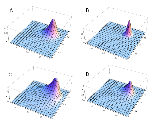
Figure 1: Profile of the integral kernel $n^{-1}\Big{|}K_{n}^{\alpha}(z,w)\Big{|}$ for fixed $z=0.3+i0.4$ as a function of $w=x+iy$. We show distinct values of $\alpha$ and $n$. One can see that the kernel presents a peak that is sharped with the increase of $n$. This behavior persists for all $\alpha\geq 2$. The distinct values of $\alpha$ are $\alpha=4$ in (A,B) and $n=50,200$ and $\alpha=8$ for $n=50,200$ in (C,D).

Asymptotic expansion for the integral kernel: We wish to obtain an asymptotic expression for the integral kernel $K_{n}^{\alpha}$. We are concerned with the behavior of the integral kernel for all $w$ in a vicinity of $z$, only the values of $w$ close $z$ gives a relevant contribution. We shall investigate the behavior of $K_{n}^{\alpha}$ in the region

$$\Delta_{\alpha}:=\Big{\{}z,w\in supp(\rho):\left|\arg z-\arg w\right|<\frac{2\pi}{\alpha}\Big{\}},$$

where $argz$ stands for the argument of the complex number $z$. We shall explain this particular choice latter on. For now it is important that $\Delta_{\alpha}$ contains the peak of $K_{n}^{\alpha}(z,w)$.

In the vicinity $\Delta_{\alpha}$ we can approximate Eq. (8) by an integral and then solve it by means of the steepest descent method. Proceeding in this way, we obtain an asymptotic expansion for the integral kernel. The technical details of this analysis shall be given elsewhere. The asymptotic expansion reads

$$n^{-1}K_{n}^{\alpha}(z,w)=\left\{\begin{array}[]{lll}n^{-1}\widehat{K}_{n}^{\alpha}(z,w)\Big{(}1+o(1)\Big{)}&&\text{if }(z,w)\in\Delta_{\alpha}\\ 0&&\text{otherwise}\end{array}\right.$$ (9)

with the leading part of the asymptotic expansion being

$$\frac{1}{n}\widehat{K}_{n}^{\alpha}(z,w)=\frac{\alpha^{2}}{4\pi}(z\overline{w})^{\frac{\alpha}{2}-1}\exp\Big{\{}n[(z\overline{w})^{\frac{\alpha}{2}}-\frac{|z|^{\alpha}}{2}-\frac{|w|^{\alpha}}{2}]\Big{\}}.$$

Now it becomes clear the behavior seen in Fig. (1). Since $2\mbox{Re}(z\bar{w})^{\alpha/2}\leq|z|^{\alpha}+|w|^{\alpha}$, being equal only if $z=w$, with the increase of $n$, $K_{n}^{\alpha}$ converges to zero exponentially fast whenever $z\not=w$.

The $o(1)$ behavior of the asymptotic expansion can be seen by introducing the quantity

$$R_{n}^{\alpha}=\displaystyle\max_{z,w\in supp(\rho)}\left|n^{-1}K_{n}^{\alpha}(z,w)-n^{-1}\widehat{K}_{n}^{\alpha}(z,w)\right|,$$

which gives the largest value of the difference between the two kernels in $\Delta_{\alpha}.$ In Fig. (2) we depict $R_{n}^{\alpha}$ as a function of $n$ for different values of $\alpha$. One can clearly see the behavior $o(1)$ of $R_{n}^{\alpha}$.

Outside the region $\Delta_{\alpha}$ the quantity $n^{-1}\widehat{K}_{n}^{\alpha}$ may differ from $n^{-1}K_{n}^{\alpha}$. $|\widehat{K}_{n}^{\alpha}(z,w)|$ has a term $\exp\{n(z\bar{w})^{\alpha/2}\}$, whose absolute value is a periodic function of period of the argument $(z\bar{w})$. To see this we write again $z=re^{i\theta}$ and $w=se^{i\xi}$, which yields

$$\left|\exp\{n(z\bar{w})^{\alpha/2}\}\right|=\exp\{n(rs)^{\alpha/2}\cos[\alpha(\theta-\xi)/2]\}.$$

As a consequence other peaks may occur in an angular distance $4\pi/\alpha$ far apart from the main peak localized in $\Delta_{\alpha}$.

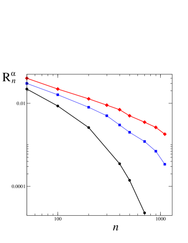
Figure 2: We depict the maximum difference $R_{n}^{\alpha}$ versus $n$. We plot $R_{n}^{\alpha}$ for three distinct values of $\alpha$, namely $\alpha=6$ (circles), $\alpha=8$ (squares) and $\alpha=11$ (diamonds). One can clearly see the $o(1)$ behavior of $R_{n}^{\alpha}$.

Rescaled integral kernel: As for the Hermitian ensembles, we shall rescale the average spacing between eigenvalues. Denoting by $D_{s}$ the disk of radius $s$ in the neighborhood of the origin, we must find a scale $g(s)$ such that the fraction of the eigenvalues in $D_{s}$ equals the area of the disk. We must have $\langle nf_{n}({D}_{g(s)})\rangle=\pi s^{2}[1+o(1)]$, with $f_{n}$ the indicator function as defined before. Explicitly, for large $n$ through the equilibrium density $\rho(re^{i\theta})$, using $z=re^{i\theta}$ we have

$$\Big{\langle}nf_{n}({D}_{g(s)})\Big{\rangle}=n\int_{0}^{2\pi}\int_{0}^{g(s)}\rho(re^{i\theta})rdrd\theta\left(1+o\left(1\right)\right).$$

solving the integral it yields $\frac{n\alpha}{2}\left(\left(g(s)\right)^{\alpha}\right)\left(1+o(1)\right)=\pi s^{2}[1+o(1)]$. The scaling function has the form

$$g\left(s\right)=\left(\frac{2\pi s^{2}}{n\alpha}\right)^{\frac{1}{\alpha}}.$$ (10)

Considering only terms of superior order in $n$ the rescaled integral kernel is given by

$$\widetilde{K}_{\alpha}\left(z,w\right)=g^{\prime}\left(z\right)\widehat{K}_{n}^{\alpha}\left(g\left(z\right),g\left(w\right)\right)\overline{g^{\prime}\left(w\right)}.$$ (11)

Note that the difference between $\widetilde{K}_{\alpha}(z,w)$ and the rescaled kernel for the Hermitian ensemble in Eq. (5) is due to the Jacobian of the coordinate change of $w\mapsto g(w)$ in the complex plane. After some manipulations the rescaled kernel reads

$$\widetilde{K}_{\alpha}(z,w)=\frac{2}{\alpha}e^{\frac{2\pi}{\alpha}\left(z\overline{w}-\frac{|z|^{2}}{2}-\frac{|w|^{2}}{2}\right)}.$$ (12)

Hence, the rescaled integral kernel, unlike the rescaled kernel for Hermitian ensembles, still carries peculiarities of the potential. Therefore, the concept of universality used for Hermitian ensembles cannot be directly extrapolated to normal ensembles. The question then turns to whether there is a scheme to obtain a universal integral kernel and consequently a universal eigenvalue statistics.

Conformal Universality: In the following, we shall show that there is a conformal map $\varphi$ such that

$$\widehat{K}_{n}^{\alpha}\overset{\varphi}{\longrightarrow}K,$$

where $K$ does not depend on the potential $V_{\alpha}$ and, in this sense, is a universal kernel. The universal kernel

$$K(z,w)=\frac{1}{\pi}e^{z\overline{w}-\frac{\left|z\right|^{2}}{2}-\frac{\left|w\right|^{2}}{2}}.$$ (13)

The conformal map $\varphi:\Sigma_{\alpha}(z)\longrightarrow\mathbb{C}$ reads

$$\varphi(w)=\sqrt{n}w^{\frac{\alpha}{2}}.$$

where $\Sigma_{\alpha}(z)=\{w\in\mathbb{C}:\left|\arg z-\arg w\right|<2\pi/\alpha\}$. The explicit relation between of integral kernels reads

$$\widehat{K}_{n}(z,w)=\varphi^{\prime}(z)K(\varphi(z),\varphi(w))\overline{\varphi^{\prime}(w)}.$$ (14)

Since $\varphi$ is a conformal transformation, we have

$$K(z,w)\overset{\varphi^{-1}}{\longrightarrow}\widehat{K}_{n}^{\alpha}(z,w)$$

where $\varphi^{-1}(w)=(w/n)^{2/\alpha}$ maps $\mathbb{C}$ into $\Sigma_{\alpha}(z)$. Thus, we conclude that the family of potentials $V_{\alpha}(z)=|z|^{\alpha}$ is conformally universal.

It is remarkable the fact that $\varphi^{-1}$ is intimately connected to unitary rescaling $g$. Introducing $u(w)=\sqrt{\alpha/2\pi}w$, we may write

$$g(w)=(\varphi^{-1}\circ u^{-1})(w),$$

where $u(w)$, acting as a rescaling of the complex plane, may stretch or shrink the distances depending on $\alpha$. Hence, the unitary rescaling $g$ is associated with the universal behavior of the ensemble after a proper rescaling of the complex plane.

Our results have also shown that for normal ensembles there is a distinction between $\widetilde{K}_{\alpha}$ and the universal kernel $K(z,w)$. Remarkably, the relation between $K$ and $\widetilde{K}_{\alpha}$ is realized by a rescaling of the complex plane through the conformal map $u(z)=\sqrt{\frac{\alpha}{2\pi}}z.$ The explicit relation reads

$$\widetilde{K}_{\alpha}(z,w)=u^{\prime}(z)K(u(z),u(w))\overline{u^{\prime}(w)}.$$ (15)

The difference between $K$ and $\widetilde{K}^{\alpha}$ is not observed in the Hermitian case. In the normal case the difference can be heuristically explained by the difference in the dimension of the eigenvalues. For the Hermitian case the influence of the Coulomb repulsion seems to be much more relevant than for the normal ensemble. Moreover, the equilibrium disposition of the eigenvalues varies with the parameter $\alpha$ due to the many possible stable crystalline structures.

In summary, we have shown that the concept of universality used for Hermitian ensembles cannot be direct extrapolated to normal ensembles. We have considered a model for random normal ensemble, where the potential is given by a radially symmetric function depending only on one $parameter$. We have shown that the rescaling of the average distance between the eigenvalues to the unity, unlike for Hermitian ensembles, does not lead to a universal eigenvalue statistics. To overcome this difficult, we have put forward a new concept of universality for normal ensembles, which we called conformal universality. We have shown that the rescaled integral kernel $K_{n}^{\alpha}(z,w)$ can be obtained by conformal transformations from a universal kernel $K(z,w)$. Our result shows that the intricate relationship between conformal geometry, revealed in the recent works Wiegman ; Zabrodin , might play an even more important role than previously thought. It is wishful to extend the procedure adopted here to general potentials.

We are in debt with Prof. Dr. W. F. Wreszinski and D. B. Liarte for a critical and detailed reading of the manuscript. We would like to acknowledge the financial of the Brazilian agencies FAPESP (TP) and CNPq (AMV and DHUM).

References

- (1) F. Haake, Quantum Signatures of Chaos, 2nd Ed., Springer-Verlag Berlin Heidelberg New York (2004) .
- (2) V.V. Sokolov and V.G. Zelevinsky, Nucl. Phys. A 504, 562 (1989); F. Haake, F. Izrailev, N. Lehmann, D. Saher, and H.J. Sommers, Z. Phys. B 88, 359 (1992); M. Müller, F.M. Dittes, W. Iskra, I. Rotter, Phys. Rev. E 52, 5961 (1995), J. Feinberg , J. Phys. A: Math. Gen. 37, 6823 (2004).
- (3) D. L. Mehta. “Random Matrices - Revised and Enlarged”. 2nd Edition. Academic Press. 1991.
- (4) J.J. M. Verbaarschot and I Zahed, Phys. Rev. Lett. 70, 3852 (1993); G. Akemann, J. Phys. A: Math Gen. 36, 3363 (2003); J. C. Osborn, Phys. Rev. Lett 93, 222001 (2004).
- (5) P. Deift. “Orthogonal Polynomials and Random Matrices: A Riemann-Hilbert Approach”. American Mathematical Society. New York University, New York (2000).
- (6) L.L. Chau and Y. Yu, Phys. Lett. A 167, 452 (1992).
- (7) R. Teodorescu, E. Bettelheim, O. Agam, A Zabrodin, P. Wiegmann, Nucl. Phys. B 704, 407 (2005).
- (8) J. Feinberg, Nucl. Phys. B 705, 403 (2005).
- (9) A. Marshakov, P. Wiegmann, A. Zabrodin, Commun. Math. Phys. 227, 131 (2002).
- (10) I.K. Kostov, I. Krichever, M. Mineev-Weinstein, P.B. Wiegmann, A Zabrodin, Math. Sci. Res. Ins. Publ. 40, 285 (2001).
- (11) L. L. Chau, O. Zaboronsky, Comm. Math. Phys. 196, 203-247 (1998).
- (12) E. Brézin and A. Zee, Nucl. Phys. B 453, 531 (1995).
- (13) A major difference in the approach of Ref. Chau and ours is Eq. (1). The authors consider a variant of it without term multiplying Tr. In this case, the eigenvalues are spread over the whole complex plane, and one cannot speak of eigenvalue density in the limit . This subtle difference makes the connection between the results extremely difficult.
- (14) P. Deift, T. Kriecherbauer, K. T.-R. McLaughlin, S. Venekides, and X. Zhou, J. Comput. Appl. Math. 133, 47-63 (2001).
- (15) E. B. Saff e V. Totik. “Logarithmic potentials with external fields”. Springer, New York-Berlin, (1997).