Dissipative breathers in rf SQUID metamaterials

F. M. Lastname

F. M. Lastname

Abstract— The existence and stability of dissipative breathers in rf SQUID (Superconducting Quantum Interference Device) arrays is investigated numerically. In such arrays, the nonlinearity which is intrinsic to each SQUID, along with the weak magnetic coupling of each SQUID to its nearest neighbors, result in the formation of discrete breathers. We analyze several discrete breather excitations in rf SQUID arrays driven by alternating flux sources in the presence of losses. The delicate balance between internal power losses and input power, results in the formation of dissipative discrete breather (DDB) structures up to relatively large coupling parameters. It is shown that DDBs may locally alter the magnetic response of an rf SQUID array from paramagnetic to diamagnetic or vice versa.

1 Introduction

The discrete breathers (DBs), which are also known as intrinsic localized modes (ILMs), belong to a class of nonlinear excitations that appear generically in discrete and spatially extended systems [1]. They are loosely defined as spatially localized, time-periodic and stable excitations, that can be produced spontaneously in a nonlinear lattice of weakly coupled elements as a result of fluctuations [2], disorded [3], or by purely deterministic mechanisms [4]. The last two decades, a large number of theoretical and experimental studies have explored the existence and the properties of DBs in a variety of nonlinear discrete systems. Nowadays, there are rigorous mathematical proofs of existence of DBs both for energy conserved and dissipative systems [5, 6], and several numerical algorithms for their accurate construction have been proposed [7, 8]. Moreover, they have been observed experimentally in a variety of systems, including solid state mixed-valence transition metal complexes [9], quasi-one dimensional antiferromagnetic chains [10], arrays of Josephson junctions [11], micromechanical oscillators [12], optical waveguide systems [13], layered crystal insulator at $300K$ [14], and proteins [15].

From the perspective of applications to experimental situations where an excitation is subjected to dissipation and external driving, dissipative DBs (DDBs) are more relevant than their energy conserved counterparts. The dynamics of DDBs is governed by a delicate balance between the input power and internal power losses. Recently, DDBs have been demonstrated numerically in discrete and nonlinear magnetic metamaterial (MM) models [16, 17]. The MMs are artificial composites that exhibit electromagnetic (EM) properties not available in naturally occuring materials. They are typically made of subwavelength resonant elements like, for example, the split-ring resonator (SRR). When driven by an alternating EM field, the MMs exhibit large magnetic response, either positive or negative, at frequencies ranging from the microwave up to the Terahertz and the optical bands [19, 20]. The magnetic response of materials at those frequencies is particularly important for the implementation of devices such as compact cavities, tunable mirrors, isolators, and converters. The nonlinearity offers the possibility to achieve dynamic control over the response of a metamaterial in real time, and thus tuning its properties by changing the intensity of the external field. Recently, the construction of nonlinear SRR-based MMs [18] gives the opportunity to test experimentally the existence of DDBs in those materials.

It has been suggested that periodic rf SQUID arrays can operate as nonlinear MMs in microwaves, due to the resonant nature of the SQUID itself and the nonlinearity that is inherent to it [21]. The combined effects of nonlinearity and discreteness (also inherent in rf SQUID arrays), may lead in the generation of nonlinear excitations in the form of DDBs [22]. In the present work we investigate numerically the existence and stability of DDBs in rf SQUID arrays. In the next section we shortly describe rf SQUID array model, which consists a simple realization of a planar MM. In section 3 we present several types of DDBs that have been constructed using standard numerical algorithms, and we discuss their magnetic response. We finish in section 4 with the conclusions.

Figure 1: Left panel: Schematic drawing of a ring-shaped rf SQUID. Middle panel: Equivalent circuit for an rf SQUID in an alternating magnetic field. Right panel: Schematic drawing of a two-dimensional orthogonal array of identical rf SQUIDs.

2 rf SQUID metamaterial model

An rf SQUID, shown schematically in the left panel of Fig. 1, consists of a superconducting ring interrupted by a Josephson junction (JJ) [23]. When driven by an alternating magnetic field, the induced supercurrents in the ring are determined by the JJ through the Josephson relations. Adopting the resistively and capacitively shunted junction (RCSJ) model for the JJ [23], an rf SQUID in an alternating field $H_{ext}\equiv H$ perpendicular to its plane is equivalent to the lumped circuit model shown in the middle panel of Fig. 1. That circuit consists of an inductance $L$ in series with an ideal Josephson element $I_{c}$ (i.e., for which $I=I_{c}\sin\phi$, where $I_{c}$ is the critical current of the JJ and $\phi$ is the Josephson phase) shunted by a capacitor $C$ and a resistor $R$, driven by an alternating flux $\Phi_{ext}(H)$.

Consider a planar rf SQUID array consisting of identical units (right panel of Fig. 1), arranged in an orthogonal lattice with constants $d_{x}$ and $d_{y}$ in the $x$ and $y$ directions, respectively. That system is placed in a uniform magnetic field $H=H_{DC}+H_{AC}\,\sin(\omega t)$, where $\omega$ is the frequency and $t$ is the temporal variable, perpendicular to the SQUID rings. The field induces a supercurrent $I_{nm}$ in the $nm-$th SQUID through the flux $\Phi_{ext}=\Phi_{DC}+\Phi_{AC}\,\sin(\omega t)$ threading the SQUID loop ($\Phi_{DC,AC}=\mu_{0}SH_{DC,AC}\omega$ is the external flux amplitude, with $\mu_{0}$ being the permeability of the vacuum and $S$ the loop area of the SQUID). The supercurrent $I_{nm}$ produces a magnetic field which couples that SQUID with its first neighbors in the $x$ and $y$ directions, due to magnetic interactions through their mutual inductances $M_{x}$ and $M_{y}$, respectively. The dynamic equations for the (normalized) fluxes $f_{nm}$ can be written in the form [22]

$$\frac{d^{2}f_{nm}}{d\tau^{2}}+\gamma\frac{df_{nm}}{d\tau}+f_{nm}+\beta\,\sin(2\pi f_{nm})-\lambda_{x}(f_{n-1,m}+f_{n+1,m})-\lambda_{y}(f_{n,m-1}+f_{n,m+1})$$

$$=[1-2(\lambda_{x}+\lambda_{y})]f_{ext},$$ (1)

where the following relations have been used

$$\tau=\omega_{0}\,t,~{}~{}\omega_{0}=1/\sqrt{L\,C},~{}~{}f_{nm}=\Phi_{nm}/\Phi_{0},~{}~{}f_{ext}=\Phi_{ext}/\Phi_{0},~{}~{}\beta=\beta_{L}/2\pi\equiv LI_{c}/\Phi_{0}.$$ (2)

In the earlier equation, $\Phi_{0}$ is the flux quantum, $\beta_{L}$ is the SQUID parameter, $\gamma$ is the dissipation constant, and $\lambda_{x,y}$ are the coupling coefficients in the $x$ and $y$ directions, defined as $\lambda_{x,y}=M_{x,y}/L$, respectively. The time derivative of $f_{nm}$ corresponds to the voltage $v_{nm}$ across the JJ of the $nm-$th rf SQUID, i.e., $v_{nm}={df_{nm}}/{d\tau}$. The normalized external flux $f_{ext}$ is given by

$$f_{ext}=f_{DC}+f_{AC}\cos(\Omega\tau),$$ (3)

where $f_{AC}=\Phi_{AC}/\Phi_{0}$, $f_{DC}=\Phi_{DC}/\Phi_{0}$, and $\Omega=\omega/\omega_{0}$, with $\Phi_{DC}$ being a constant (DC) flux resulting from the time-independent component of the magnetic field $H$.

The dispersion for small amplitude flux waves is obtained by the substitution of $f=A\,\exp[i(\kappa_{x}n+\kappa_{y}m-\Omega\tau)]$, into the linearized Eqs. (2) for $\gamma=0$ and $f_{ext}=0$, which gives

$$\Omega_{\bf\kappa}=\sqrt{1+\beta_{L}-2(\lambda_{x}\,\cos\kappa_{x}+\lambda_{y}\,\cos\kappa_{y})},$$ (4)

where ${\bf\kappa}=(\kappa_{x},\kappa_{y})=(d_{x}\,k_{x},d_{y}\,k_{y})$. The corresponding one-dimensional (1D) SQUID array is obtained by setting $\lambda_{y}=0$, $\lambda_{x}=\lambda$, $\kappa_{x}=\kappa$, and by dropping the subscript $m$ in Eqs. (2). Typical dispersion curves $\Omega(\kappa)$ for the 1D system are shown in Fig. 2a for three different values of the coupling $\lambda$. The bandwidth $\Delta\Omega\equiv\Omega_{max}-\Omega_{min}$ decreases with decreasing $\lambda$ which leads, for $\lambda<<1$ [24], to a nearly flat band with $\Delta\Omega\simeq 2\lambda\sqrt{1+\beta_{L}}$ (and relative bandwidth $\Delta\Omega/\Omega\simeq 2\lambda$). Importantly, the group velocity $v_{g}$, which defines the direction of power flow, is in a direction opposite to the phase velocity $v_{ph}$, as it is observed in Fig. 2b.

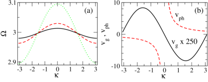
Figure 2: (a) Frequency band $\Omega$ as a function of $\kappa$ for a 1D rf SQUID array, for $\beta=1.27$, and $\lambda=-0.05$ (narrowest band, black-solid curve), $\lambda=-0.1$ (red-dashed curve), $\lambda=-0.3$ (widest band, green-dotted curve). (b) Group velocity $v_{g}$ (black-solid curve) and phase velocity $v_{ph}$ (red-dotted curve), for a 1D rf SQUID array with $\beta=1.27$ and $\lambda=-0.1$.

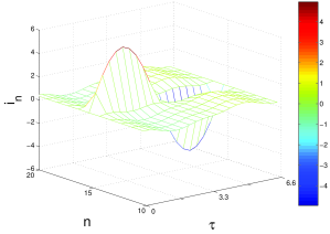
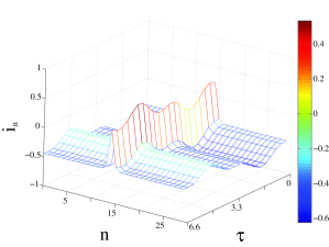
Figure 3: Time evolution of dissipative breathers during one period, for $\lambda=-0.1$, $T_{b}=6.6$, $\gamma=0.001$, $\beta=1.27$, and (right panel) $f_{DC}=0.5$, $f_{AC}=0.2$ - low-amplitude breather; (left panel) $f_{DC}=0$, $f_{AC}=0.6$ - high-amplitude breather. Only part of the array ($N=30$) is shown for clarity.

3 Dissipative breathers and magnetic response

For the generation of DDBs in rf SQUID arrays, we use the algorithm developed by Marin et. al. [7]. With that algorithm, we can construct low- and high-amplitude DDBs up to some maximum value of the coupling, $\lambda_{max}$, which generally depends on the external flux amplitudes $f_{AC}$ and $f_{DC}$ [22]. Both the central site and the background of those DDBs are oscillating with frequency $\Omega_{b}=2\pi/T_{b}=\Omega$, i.e., the same as that of the external flux, $\Omega$. Typical single-site bright DDBs of both low- and high-amplitude are shown in Fig. 3 (right and left panels, respectively), where the spatio-temporal evolution of the induced currents $i_{n}$ ($n=1,2,3,...,N$) are shown during one DDB period $T_{b}$. We should note the non-sinusoidal time-dependence of the oscillations in both panels of Fig. 3. The linear stability of DDBs is addressed through the eigenvalues of the Floquet matrix (Floquet multipliers). A DDB is linearly stable when all its Floquet multipliers $m_{i},~{}i=1,...,2N$, lie on a circle of radius $R_{e}=\exp(-\gamma T_{b}/2)$ in the complex plane. The DDBs shown in Fig. 3 are indeed linearly stable. Moreover, those DDBs were let to evolve for large time intervals (i.e., more than $10^{5}~{}T_{b}$) without any observable change in their shapes. With the same algorithm, we can also construct 2D dissipative breathers. A snapshot of such a DDB taken at maximum amplitude of the central site is shown in the left panel of Fig. 4.

The normalized flux through the $nm-$th SQUID can be casted in the form

$$\beta\,i_{nm}=f_{nm}^{loc}-f_{ext}^{eff},$$ (5)

where

$$f_{nm}^{loc}=f_{nm}-\lambda_{x}(f_{n-1,m}+f_{n+1,m})-\lambda_{y}(f_{n,m-1}+f_{n,m+1}),\qquad f_{ext}^{eff}=[1-2(\lambda_{x}+\lambda_{y})]f_{ext}.$$ (6)

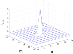
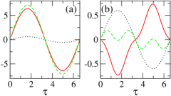
Figure 4: Left panel: A snapshot of a two-dimensional dissipative discrete breather (DDB) for $\lambda_{x}=\lambda_{y}=-0.1$ and the other parameters as in the left panel of Fig. 3. Right panel: Temporal evolution of $\beta\,i_{n}$ (red-solid curve), $f_{n}^{loc}$ (green-dashed curve), and $f_{ext}$ (black-dotted curve) during one period $T_{b}$, for (a) the central site of the DDB shown in the left panel ($n=m=n_{b}=N/2$); (b) the site with $n=m=7$ of the DDB shown in the left panel.

After division by the area of the unit cell $d^{2}$ of the 2D array, the terms $f_{ext}^{eff}$, $f_{nm}^{loc}$, and $\beta\,i_{nm}$ in Eq. (5) can be interpreted as the effective external field, the local magnetic induction at the $nm-$th cell, and the magnetic response at the $nm-$th cell, respectively. The temporal evolution of $\beta\,i_{nm}$, $f_{nm}^{loc}$, and the external field $f_{ext}$, are shown in the right panel of Fig. 4, for two different sites of the 2D DDB shown in the left panel of Fig. 4: the central DDB site at $n=m=n_{b}=N/2$, and the site located at $n=m=7$ (Figs. (a) and (b) of the right panel of Fig. 4, respectively). We observe that in the cell corresponding to the central DDB site the magnetic response is in phase with the applied field providing a strong paramagnetic response, while in the cell corresponding to the site located in the background the magnetic response is in anti-phase with the applied field providing moderate diamagnetic response. Thus, the local magnetic induction is sharply peaked at the central DDB site, as can be inferred by comparing the green-dashed curves in (a) and (b) in the right panel of Fig. 4.

4 Conclusion

In conclusion, we have shown using standard numerical methods that periodic rf SQUID arrays in an alternating external flux support low- and high-amplitude linearly stable DDBs. Those DDBs are not destroyed by increasing the dimensionality from one to two. Thus, we have constructed several linearly stable DDB excitations both for 1D and 2D rf SQUID arrays, which may alter locally the magnetic response of the arrays. Planar SQUID arrays similar to those described here have been actually constructed and studied with respect to the ground state ordering of their magnetic moments [24]. Thus, the above theoretical predictions are experimentally testable.

Bibliography

- [1] Flach, S. and Gorbach, A. V., “Discrete breathers - Advances in theory and applications”, Phys. Rep. Vol. 467, No. 1-3, 1–116, 2008.
- [2] Peyrard, M., ”The pathway to energy localization in nonlinear lattices”, Physica D Vol. 119, No. 1-2, 184–199, 1998.
- [3] Rasmussen, K. Ø., Cai, D., Bishop, A. R., and Grønbech-Jensen, N., “Localization in a nonlinear disordered system”, Europhys. Lett. Vol. 47, No. 4, 421–427, 1999.
- [4] Hennig, D., Schimansky-Geier, L. and Hänggi, P., “Self-organized, noise-free escape of a coupled nonlinear oscillator chain”, Europhys. Lett. Vol. 78, No. 2, 20002-p1–20002-p6, 2007.
- [5] MacKay, R. S., and Aubry, S., “Proof of existence of breathers for time - reversible or Hamiltonian networks of weakly coupled oscillators”, Nonlinearity, Vol. 7, No. 6, 1623–1643, 1994.
- [6] Aubry, S., “Breathers in nonlinear lattices: Existence, linear stability and quantization”, Physica D, Vol. 103, No. 1-4, 201–250, 1997.
- [7] Marín, J. L. and Aubry, S., “Breathers in nonlinear lattices: numerical calculation from the anticontinuous limit”, Nonlinearity, Vol. 9, No. 6, 1501–1528, 1996.
- [8] Marín, J. L., Falo, F., Martínez, P. J. and Floría, L. M., “Discrete breathers in dissipative lattices”, Phys. Rev. E, Vol. 63, No. 6, 066603-1–066603-12, 2001.
- [9] Swanson, B. I., Brozik, J. A., Love, S. P. Strouse, G. F., Shreve, A. P., Bishop, A. R., Wang, W.-Z. and Salkola, M. I., “Observation of intrinsic localized modes in a discrete low-dimensional material”, Phys. Rev. Lett., Vol. 82, No. 16, 3288–3291, 1999.
- [10] Schwarz, U. T., English, L. Q. and Sievers, A. J., “Experimental generation and observation of intrinsic localized spin wave modes in an antiferromagnet”, Phys. Rev. Lett., Vol. 83, No. 1, 223–226, 1999.
- [11] Trías, E., Mazo, J. J. and Orlando, T. P., “Discrete breathers in nonlinear lattices: Experimental detection in a Josephson array”, Phys. Rev. Lett., Vol. 84, No. 4, 741–744, 2000.
- [12] Sato, M., Hubbard, B. E., Sievers, A. J., Ilic, B., Czaplewski, D. A. and Graighead, H. G., “Observation of locked intrinsic localized vibrational modes in a micromechanical oscillator array”, Phys. Rev. Lett., Vol. 90, No. 4, 044102-1–044102-4, 2003.
- [13] Eisenberg, H. S., Silberberg, Y., Morandotti, R., Boyd, A. R. and Aitchison, J. S., “Discrete spatial optical solitons in waveguide arrays”, Phys. Rev. Lett., Vol. 81, No. 16, 3383–3386, 1998.
- [14] Russell, F. M. and Eilbeck, J. C., “Evidence for moving breathers in a layered crystal insulator at 300 K”, Europhys. Lett., Vol. 78, No. 1, 10004-p1–10004-p5, 2007.
- [15] Edler, J., Pfister, R., Pouthier, V., Falvo, C. and Hamm, P., “Direct observation of self-trapped vibrational states in Helices”, Phys. Rev. Lett., Vol. 93, No. 10, 106405-1–106405-4, 2004.
- [16] Lazarides, N., Eleftheriou, M. and Tsironis, G. P., “Discrete breathers in nonlinear magnetic metamaterials”, Phys. Rev. Lett., Vol. 97, No. 15, 157406-1–157406-4, 2006.
- [17] Eleftheriou, M., Lazarides, N. and Tsironis, G. P., “Magnetoinductive breathers in metamaterials”, Phys. Rev. E, Vol. 77, No. 3, 036608-1–036608-13, 2008.
- [18] Shadrivov, I. V., Kozyrev, A. B., van der Weide, D. W. and Kivshar, Yu. S., “Tunable transmission and harmonic generation in nonlinear metamaterials”, Appl. Phys. Lett., Vol. 93, No. 16, 161903-1–161903-3, 2008.
- [19] Linden, S., Enkrich, C., Dolling, G., Klein, M. W., Zhou, J., Koschny, T., Soukoulis, C. M., Burger, S., Schmidt, F. and Wegener, M., “Photonic metamaterials: magnetism at optical frequencies”, IEEE J. Selec. Top. Quant. Electron., Vol. 12, No. 6, 1097–1105, 2006.
- [20] Shalaev, V. M., “Optical negative-index metamaterials”, Nature Photonics, Vol. 1, No. 1, 41–48, 2007.
- [21] Lazarides, N. and Tsironis, G. P., “rf superconducting quantum interference device metamaterials”, Appl. Phys. Lett., Vol. 90, No. 16, 163501-1–163501-3, 2007.
- [22] Lazarides, N., Tsironis, G. P. and Eleftheriou, M., “Dissipative discrete breathers in rf SQUID metamaterials”, Nonlin. Phen. Compl. Syst., Vol. 11, No. 2, 250–258, 2008.
- [23] Likharev, K. K., Dynamics of Josephson Junctions and Circuits, Gordon and Breach, Philadelphia, 1986.
- [24] Kirtley, J. R., Tsuei, C. C., Ariando, Smilde, H. J. H. and Hilgenkamp, H., “Antiferromagnetic ordering in arrays of superconducting rings”, Phys. Rev. B, Vol. 72, No. 21, 214521-1–214521-11, 2005.