Comparing Single and Multiobjective Evolutionary Approaches to the Inventory and Transportation Problem

Abstract

EVITA, standing for Evolutionary Inventory and Transportation Al-gorithm, is a two-level methodology designed to address the Inventory and Transportation Problem (ITP) in retail chains. The top level uses an evolutionary algorithm to obtain delivery patterns for each shop on a weekly basis so as to minimise the inventory costs, while the bottom level solves the Vehicle Routing Problem (VRP) for every day in order to obtain the minimum transport costs associated to a particular set of patterns.

The aim of this paper is to investigate whether a multiobjective approach to this problem can yield any advantage over the previously used single objective approach. The analysis performed allows us to conclude that this is not the case and that the single objective approach is in general preferable for the ITP in the case studied. A further conclusion is that it is useful to employ a classical algorithm such as Clarke & Wright’s as the seed for other metaheuristics like local search or tabu search in order to provide good results for the Vehicle Routing Problem.

1 Introduction

Given a retail chain and a central depot that supplies it, both belonging to the same company, we define the Inventory and Transportation Problem as that whose objective is to minimise the costs of both inventory and transportation, subject to a number of constraints imposed at the shop level.

In previous work (Esparcia-Alcázar et al., 2006a, ; Esparcia-Alcázar et al., 2006b, ; Esparcia-Alcázar et al., 2007a, ; Esparcia-Alcázar et al., 2007b, ; Esparcia-Alcázar et al.,, 2009) we employed a single objective approach to this problem, which aimed at minimising the total weekly cost calculated as the sum of the inventory and transportation costs. The purpose of the current work is to evaluate the convenience of adopting a multiobjective approach to the problem. Although it is true that the aim of the ITP is to minimise the global cost and this is calculated by simply adding the costs of inventory and transport (both measured in currency units), it is no less true that the minimisation of both costs are contradictory objectives since, as was stated above, reducing the cost of transport implies increasing the cost of inventory and vice versa. For this reason it is possible that a multiobjective approach will obtain better results in this problem, and this is what we set out to investigate.

With this aim in mind we have carried out an extensive series of experiments using the eight instances used in (Esparcia-Alcázar et al.,, 2009), plus two new ones. The set of restrictions, consisting of the characteristics of the vehicles employed and the working hours of the drivers (see Table 7), plus the parameter configuration of the evolutionary algorithm are kept as in that work.

In the multiobjective approach we have used the NSGA-II algorithm (Deb et al.,, 2000), which is described in more detail in Appendix I.

A further objective is related to the fact that the choice of the algorithm that yields the transportation routes (the VRP solver) can play a significant part in the performance of the whole algorithm (Esparcia-Alcázar et al., 2006a, ). Here we will employ improved versions of three different algorithms that have been employed in the literature for solving the VRP and will compare them on the selected problem instances, with the aim to determine whether there is a relation between the instance characteristics and the performance of the VRP solver. The VRP algorithms studied are improved variants of the three that obtained best results in (Esparcia-Alcázar et al.,, 2009): tabu search (Cordeau et al.,, 1997), ant colony optimisation (Dong and Xiang,, 2006) and a classical VRP solving technique, Clarke and Wright’s algorithm (Clarke and Wright,, 1964).

The rest of the paper is structured as follows. Section 2 provides background on the problem; it contains a summary of the state of the art in this and related problems and a detailed description of the ITP. The top and lower levels of the algorithm are described in Sections 3 and 4, the latter containing the details of the three VRP solvers employed. The experimental setup is given in Section 5, with results and analysis thereof contained in Section 6. Finally, Section 7 presents the conclusions and outlines future areas of research.

2 Problem background

The ITP deals with the management of two different aspects of retail chain logistics, inventory costs and transportation costs, which have both received lots of attention in the logistics literature. Here we will describe how they have been addressed in the past and what aspects are particularly relevant to our case.

2.1 The Vehicle Routing Problem

The Vehicle Routing Problem (VRP) consists on finding an optimal set of delivery routes from a depot to a set of customers to serve (Toth and Vigo,, 2001). The routes must start and finish in the depot and each customer must be served by one and only one vehicle, which means a customer cannot be contained in more than one route. Different versions of the problem have slightly different objectives or ways to define optimality: it can refer to finding the minimum cost, employing minimum time, minimum number of delivery vehicles or combinations of these and other factors.

Amongst these variants of the problem the most popular is the capacitated VRP, or CVRP, which refers to the fact that each delivery vehicle has a limited capacity. Also popular is the VRP with time windows, or VRPTW, in which each customer must be served during a specified time interval or window.

Another variant of the VRP relevant to our problem is the periodic vehicle routing problem (PVRP), which appears when customers have established a predetermined delivery frequency and a combination of admissible delivery days within the planning horizon. The objective is to minimise the total duration of the routes, while the restrictions usually involve a limited capacity of the delivery vehicles and a maximum duration of each itinerary. See for instance, (Cordeau et al.,, 1997) and (Toth and Vigo,, 2001) for a general description of the periodic VRP.

In this paper we are concerned with the CVRP, simply referred to as VRP. The only limitation will be in the capacity of the vehicles used, and not in their number. We will also consider that the fleet is homogeneous, i.e. only one type of vehicle is used, with unique values of average velocity and capacity.

For simplicity reasons we will consider that the customers (shops in the retail chain in our case) have no time windows, i.e. the deliveries can take place at any time. However, the hours a driver can work are limited by regulations and this has to be taken into account in the time needed per delivery, as is the unloading time. Also, it should be possible to serve all customers; this means that routes from the depot to any customer and back must take less than the working hours of the driver.

Finally, we will consider that the transport cost only includes the cost per kilometer; there is no cost attached to either the time of use of the vehicle or to the number of units delivered, nor there is a fixed cost per vehicle.

2.2 Inventory and transportation management

One step beyond the VRP is the problem of optimising simultaneously the costs of inventory and transportation. In (Esparcia-Alcázar et al., 2007a, ) the reader can find a review of different approaches employed in the literature.

Amongst these, one of the most relevant to our case is the inventory routing problem (IRP), which arises when a vendor delivers a single product and implements a Vendor Inventory Management (VIM) (Çetinkaya and Lee,, 2000) policy with its clients, so that the vendor decides the delivery (time and quantity) in order to prevent the clients from running out of stock while minimising transportation and inventory holding costs (Campbell and Savelsbergh,, 2004). However, retail chains cannot be addressed in this way, as thousands of items are involved.

The work presented here focuses on the Inventory and Transportation Problem (ITP), which was first described in (Cardós and García-Sabater,, 2006) with the aim of addressing the case of retail chains. Thus, the ITP can be viewed as a generalisation of the IRP to the multiproduct case. Additionally, it can also be viewed as a variant of the PVRP described previously that includes inventory costs and a set of delivery frequencies instead of a unique delivery frequency for each shop.

The main feature that differentiates the ITP from other similar supply chain management ones addressed in the literature (Çetinkaya and Lee,, 2000; dos Santos Coelho and Lopes,, 2006; Federgruen and Zipkin,, 1984; Sindhuchao et al.,, 2005; Viswanathan and Mathur,, 1997) is that we have to decide on the frequency of delivery to each shop, which determines the size of the deliveries. The inventory costs can then be calculated accordingly, assuming a commonly-employed periodic review stock policy for the retail chain shops. Besides, for a given delivery frequency, expressed in terms of number of days a week, there can also be a number of delivery patterns, i.e. the specific days of the week in which the shop is served. Once these are established, the transportation costs can be calculated by solving the VRP for each day of the week.

Because a pattern assumes a given frequency, the problem is limited to obtaining the optimal patterns (one per shop) and set of routes (one set per day). The optimum is defined as a combination of patterns and routes that minimises the total cost, which is calculated as the sum of the individual inventory costs per shop (inventory cost) plus the sum of the transportation costs for all days of the week (transport cost). These two objectives are in general contradictory: the higher the frequency of delivery the lower the inventory cost, but conversely, a higher frequency involves higher transportation costs.

The operational constraints at the shop level are imposed by the business logic and can be listed as follows (Esparcia-Alcázar et al.,, 2009):

1. A periodic review stock policy is applied for the shop items. This means that the decision of whether to deliver to a particular shop is taken centrally and not at the shop. As a consequence, stockout is allowed.

2. Shops have a limited stock capacity.

3. The retail chain tries to fulfil backorders in as few days as possible, so there is a lower bound for delivery frequency, which depends on the target client service level.

4. The expected stock reduction between replenishments (deliveries) cannot be too high in order to avoid two problems: (a) the unappealing empty-shelves aspect of the shop just before the replenishment; and (b) replenishment orders too large to be placed on the shelves by the shop personnel in a short time compatible with their primary selling activity.

5. Conversely, the expected stock reduction must be high enough to perform an efficient allocation of the replenishment order.

6. As a consequence of points 2 to 5 above, not all frequencies are admissible for all shops; in general, very high and very low frequencies are undesirable. For instance, frequency 1 (one delivery per week) is not applicable to most shops.

7. Sales are not uniformly distributed over the time horizon (week), tending to increase over the weekend. Hence, in order to match deliveries to sales, only a given number of delivery patterns are allowed for every feasible frequency. For instance, a frequency-2 pattern such as (Mon, Fri) is admissible, while another of the same frequency such as (Mon, Tues) is not.

8. Although we are dealing with thousands of items, the load is containerised; hence, the size of the deliveries is expressed as an integer, representing the number of roll-containers.

Thus, to summarise, our task involves finding:

• The optimal set of patterns, $\mathcal{P}_{opt}$, with which all shops can be served. A pattern $p$ represents a set of days in which a shop is served which implies a delivery frequency (expressed as number of days a week) for the shop

• The optimal routes for each day of the working week, by solving the VRP for the shops allocated to that day by the corresponding pattern

2.3 Objective functions in EVITA

EVITA operates in two levels: the lower one deals exclusively with the transportation costs per day and the top one incorporates these and the inventory costs into the total costs.

In the single objective case, the optimum is defined as the solution that minimises the total cost, given by the function

$$f=TotalCost=InventoryCost+TransportCost$$ (1)

In the multiple objective approach, we will deal with two separate cost functions:

$$f_{i}=InventoryCost$$ (2)

$$f_{t}=TransportCost$$ (3)

However, we will still use the total cost defined for the single objective case to compare the results between multi and monoobjective solutions. The reason is that the company is interested in spending less, irrespective of where the reduction comes from, and, at the end of the day, both costs come in euros.

Inventory costs are computed from the patterns for each shop by taking into account the associated delivery frequency and looking up the inventory cost per shop in the corresponding table. An example of the latter is given in Table 1.

Table 1: Inventory cost (in Euro) and size of the deliveries per shop (expressed in roll containers) depending on the delivery frequency (in days). Missing data corresponds to frequencies that are not admissible for each shop.

	Inventory cost					Delivery size
	(€)					(roll containers)
Shop #	Frequency (days)					Frequency (days)
	1	2	3	4	5	1	2	3	4	5
1	-	-	-	336	325	-	-	-	2	2
2	-	-	-	335	325	-	-	-	2	2
$\cdots$	$\cdots$	$\cdots$	$\cdots$	$\cdots$	$\cdots$	$\cdots$	$\cdots$	$\cdots$	$\cdots$
N	-	311	293	286	284	-	3	2	2	1

For instance, let us assume that shop N was assigned a pattern of frequency 4; we would look up in the table the inventory cost for the shop at that frequency, which is 286€. Proceeding in the same way with all shops and adding up the results we would obtain the total inventory cost.

Transport costs are obtained by solving the VRP with one of the algorithms under study. The demands (size of deliveries) of each shop would also be taken from Table 1. In the example above, for shop N at frequency 4 the delivery size is 2 roll containers.

Problem data is freely available from our group website: http://casnew.iti.es/

3 The top level: Evolutionary Algorithm

The top level in EVITA is an evolutionary algorithm in which a population of individuals (candidate solutions) undergoes evolution following Darwinian principles. Each individual is a set of patterns $\mathcal{P}$ represented as a vector of length equal to the number of shops to serve ($nShops$),

$$P=(p_{1},p_{2},\cdots,p_{nShops})$$

and whose components $p_{i},~{}1\leq p_{i}\leq 2^{d}-1$, $i\in\{1\dots nShops\}$ are integers representing a particular delivery pattern, where $d$ is the number of days in the working week.

The relationship between patterns and delivery days is made at bit level. Each pattern is formed by $d$ bits and each day corresponds to one bit: 1 means that the store is visited that day and 0 that it is not. In our case the working week has 5 days (Monday to Friday) so $d=5$. Hence patterns are coded by the rightmost 5 bits of the integer value. For instance pattern 21, i.e. 10101 in binary, corresponds to deliveries on Monday, Wednesday and Friday.

The total number of possible patterns is $2^{d}-1$; in our case $2^{5}-1=31$, so patterns range from 1 to 31 or, alternatively, from 00001 to 11111 (obviously pattern 00000, i.e. not delivering any day, is not admissible). However, as was stated in Subsection 2.2, not all patterns are suitable for all shops. Hence, $p_{i}$ must be contained in the set of admissible patterns, $p_{i}\in$ $\mathcal{P}$_adm. The elements in $\mathcal{P}$_adm are given in Table 2.

Table 2: The admissible patterns and their respective frequencies. The 1 represents that the shop is served on that day, the 0 that it is not. As a consequence of the business logic, we will only consider 11 patterns out of the 31 that are possible.

Pattern Id.	Frequency (days)	Mon	Tues	Wed	Thurs	Fri
5	2	0	0	1	0	1
9	2	0	1	0	0	1
10	2	0	1	0	1	0
11	3	0	1	0	1	1
13	3	0	1	1	0	1
17	2	1	0	0	0	1
18	2	1	0	0	1	0
21	3	1	0	1	0	1
23	4	1	0	1	1	1
29	4	1	1	1	0	1
31	5	1	1	1	1	1

A point to note is that although the binary representation of the patterns is convenient in order to figure out what delivery days are associated to a pattern and also for calculating its corresponding frequency, in the genetic algorithm we will be considering the integer values only.

The details of the top level evolutionary algorithm are given in Table 3. The pseudo-code for the evaluation function is given in Algorithm 1.

Procedure Evaluate

input:

Chromosome $\{p_{1},\dots,p_{nShops}\}$,

problem data tables

$costPerKm$

output: Fitness

[Calculate inventory cost]

InventoryCost = 0

for $i=1$ to $nShops$

Look up frequency $f_{i}$ for pattern $p_{i}$

Look up cost $c_{i}$ for shop $i$ and frequency $f_{i}$

$InventoryCost+=c_{i}$

[Calculate transportation cost]

$day=Monday$;

$totalDistance=0$

repeat

Identify shops to be served on $day$

Run VRP solver to get $dayDistance$

$totalDistance+=dayDistance$

$day++$

until $day=lastWorkingDay$;

$TransportCost=totalDistance*costPerKm$

if multiobjective

return $InventoryCost,~{}TransportCost$

[Calculate total cost]

$TotalCost=InventoryCost+TransportCost$

return $TotalCost$

end procedure;

Algorithm 1 Evaluation function.

Table 3: Configuration of the top-level evolutionary algorithm employed (both mono and multiobjective).

Encoding	The gene $i$ represents the pattern for shop $i$.
	The chromosome length is equal to the number of shops ($nShops$).
Selection	Tournament in 2 steps. To select each parent, we take $tSize$ individuals chosen randomly and select the best.
	For the single objective algorithm the best 10 individuals of each generation are preserved as the elite.
Evolutionary operators	2 point crossover and 1-point mutation.
	The mutation operator changes the pattern for 1 shop in the chromosome.
Termination criterion	Terminate when the total number of generations (including the initial one) equals 100.
Fixed parameters	Population size, $popSize=100$
	Tournament size, $tSize=2$
	Mutation probability, $pM=0.2$
	Crossover probability, $pC=1$

4 Lower level: Solving the VRP

The calculation of the fitness of an individual requires an algorithm to solve the VRP (a VRPsolver). In this work three algorithms have been tested for this purpose, namely:

• CWLS, the classical Clarke and Wright’s algorithm (Clarke and Wright,, 1964) enhanced with local search, which is presented in subsection 4.1

• ACO, a bioinspired ant colony optimisation algorithm (Dorigo and Stutzle,, 2004), described in subsection 4.2, and

• CWTS, tabu search (Glover and Kochenberger,, 2002) seeded with a solution obtained by Clarke and Wright algorithm, as described in subsection 4.3

In (Esparcia-Alcázar et al.,, 2009) we also employed a fourth algorithm as VRPsolver, evolutionary computation. However, the results obtained there were not very promising, which is why it has been omitted in this study.

4.1 Clarke and Wright’s algorithm

Clarke and Wright’s algorithm (Clarke and Wright,, 1964) is based on the concept of saving, which is the reduction in the traveled length achieved when combining two routes. We employed the parallel version of the algorithm, which works with all routes simultaneously.

Due to the fact that the solutions generated by the C&W algorithm are not guaranteed to be locally optimal with respect to simple neighbourhood definitions, it is almost always profitable to apply local search to attempt and improve each constructed solution. For this purpose we designed a simple and fast local search method, which consists on performing 2-interchanges on the solution obtained by the C&W algorithm. Every possible pair of shops is exchanged, first between shops in the same route and then between shops in different routes. If at any time an invalid route is generated (because the restrictions on time or capacity are violated) the depot is inserted where required in the route. The best neighbour solution will be the one with a lower associated transport cost.

This combination of C&W’s algorithm with local search is what we have termed CWLS, the pseudo-code for both can be found in Algorithms 4 and 5.

4.2 Ant Colony Optimisation

Some ant systems have been applied to the VRP (see for instance (Coltorti and Rizzoli,, 2007; Gendreau et al.,, 2002)) with various degrees of success. Ant algorithms are derived from the observation of the self-organized behavior of real ants (Dorigo and Stutzle,, 2004). The main idea is that artificial agents can imitate this behavior and collaborate to solve computational problems by using different aspects of ants’ behavior. One of the most successful examples of ant algorithms is known as “ant colony optimisation”, or ACO, which is based on the use of pheromones, chemical products dropped by ants when they are moving.

Each artificial ant builds a solution by choosing probabilistically the next node to move to among those it has not visited yet. The choice is biased by pheromone trails previously deposited on the graph by other ants and some heuristic function. Also, each ant is given a limited form of memory in which it can store the partial path it has followed so far, as well as the cost of the links it has traversed. This, together with deterministic backward moves, helps avoiding the formation of loops (Dorigo and Stutzle,, 2004).

In this work we employed a variant of ACO described by Xiang-pei et al., (2006) which differs from the original ACO algorithm in three aspects: (1) the way the pheromone matrix is updated, (2) the transition function and (3) that $\lambda$-interchanges are used instead of local search.

Two ways of updating the pheromone matrix $\tau$ are defined: local updating and a posteriori updating (i.e. taking place after all ants have built their solutions). The former consists of adding $1/d_{i,j}$ to each element $\tau_{i,j}$ of the pheromone matrix, with $d_{i,j}$ being the distance between shops $i$ and $j$. The latter is given by Equation 4. Here the best path built in iteration $t$ receives a reinforcement while the worst path is reset to the initial pheromone value, $\tau_{0}$.

$$\tau_{i,j}=\left\{\begin{array}[]{ll}\tau_{i,j}(\rho+\frac{1-\rho}{minCost_{t}})&\parbox[c][34.14322pt][c]{213.39566pt}{if $(i,j$) is an arc visited by the \emph{best} ant\\ in iteration $t$}\\ \tau_{0}&\parbox[c][34.14322pt][c]{213.39566pt}{if $(i,j)$ is an arc visited by the \emph{worst} ant \\ in iteration $t$}\\ \end{array}\right.$$ (4)

where $minCost_{t}$ is the minimum cost obtained in iteration $t$ and the value of $\rho$ is automatically corrected in each iteration, as follows,

$$\rho_{t}=\left\{\begin{array}[]{ll}0.95\rho_{t-1}&\hbox{if }0.95\rho_{t-1}<\rho_{min}\\ \rho_{min}&\hbox{otherwise}\\ \end{array}\right.$$ (5)

The second difference with respect to the original ACO is the transition function. In our ACO an ant located at shop $i$ will select as its next shop $j$ the one given by Equation 6, with probability $p_{t}$,

$$j=argmax_{S}[\tau_{i,j}]^{\alpha}[\eta_{i,j}]^{\beta}[\mu_{i,j}]^{\gamma}$$ (6)

where $S$ is the list of shops not visited yet, $\tau$ is the pheromone matrix, $\eta$ is the heuristic function,

$$\eta_{i,j}=\frac{1}{d_{i,j}}$$

and finally,

$$\mu_{i,j}=d_{i,0}+d_{0,j}-d_{i,j}$$

corresponds to the concept of saving used in Clarke & Wright’s algorithm, with shop 0 being the depot. Alternatively, the next shop $j$ will be uniformly selected at random from $S$.

The parameters $\alpha$, $\beta$ and $\gamma$ (whose sum does not necessarily equal 1) measure the relative importance of each component. The probability value $p_{t}$ is dynamically adjusted at runtime in a similar way as for $\rho_{t}$, following Equation 7.

$$p_{t}=\left\{\begin{array}[]{ll}0.95p_{t-1}&\qquad\hbox{if }\quad 0.95~{}p_{t-1}\geq p_{min}\\ p_{min}&\qquad\hbox{otherwise}\\ \end{array}\right.$$ (7)

Finally, instead of using local search in the closest neighbours as in conventional ACO, we use $\lambda$-interchanges, a concept borrowed from the CWLS algorithm described earlier.

The pseudo-code for the ACO algorithm employed here is given in Algorithm 6, its transition function is shown in Algorithm 7 and the parameters used are given in Table 4.

Table 4: Parameters for ACO. The values were obtained by trial and error, as explained in (Martínez-García,, 2008). Notice that $\alpha$, $\beta$ and $\gamma$ do not necessarily add up to 1.

Number of Iterations	$nIters=50$
Number of Ants	$nAnts=25$
Transition function	Probability, $p_{t}$
	Initial value, $p_{0}=0.8$
	Minimum value, $p_{min}=0.1$
	Weights:
	Pheromone: $\alpha=0.2$
	Heuristics: $\beta=0.8$
	Savings: $\gamma=0.3$
Pheromones	Initial value, $\tau_{0}=0.5$
	Update factor, $\rho$
	Initial value, $\rho_{0}=1$
	Minimum value, $\rho_{min}=0.1$

4.3 Tabu Search

Tabu Search (TS) is a metaheuristic introduced by Glover and Kochenberger in order to allow Local Search (LS) methods to overcome local optima (Glover and Kochenberger,, 2002). The basic principle of TS is to pursue LS whenever a local optimum is found by allowing non-improving moves; cycling back to previously visited solutions is prevented by the use of memories, called tabu lists (Gendreau,, 1999) which last for a period given by their tabu tenure. The main TS loop is given in Algorithm 8.

To obtain the best neighbour of the current solution we must move in the solution’s neighbourhood, avoiding moving into older solutions and returning the best of all new solutions. This solution may be worse than the current solution. For each solution we must generate all possible and valid neighbours whose generating moves are not tabu. If a new best neighbour is created, the movement is inserted into the Tabu List with the maximum tenure. This movement is kept in the list until its tenure is over. The tenure can be a fixed or variable number of iterations.

The way to obtain the best neighbour is described in Algorithm 9. Table 5 lists the relevant information about the algorithm.

In order to improve over the TS algorithm used in (Esparcia-Alcázar et al.,, 2009), we considered seeding the TS with a good solution. The solution chosen as a starting point was one obtained by the C&W algorithm. Statistical analysis carried out shows that the seeded algorithm obtains significantly better results than when the initial solution is obtained at random. For this reason, in the rest of this work we have employed this improved version, which we have termed CWTS.

Table 5: Configuration for CWTS algorithm. The parameters were tuned heuristically, after several test launches. The chosen values (small value for the Tabu Tenure and large number of iterations without solution improvement) sacrifice execution time in order to obtain better solutions.

Initial solution	A solution obtained by Clarke & Wright’s algorithm
Possible moves	Swap shop $i$ with shop $j$, both in same route
	Swap shop $i$ with shop $j$, in different routes
	Create new route with shop $i$ only
Tabu tenure	12 iterations
Termination criterion	20 iterations without improvement

5 Experiments

This section is devoted to present the data we have used in the problem (subsection 5.1) and the experimental procedure we have followed (in the next subsection, 5.2).

5.1 Problem data

As explained above, we will employ a number of geographical layouts available on the web. We have selected our instances so as to achieve the maximum representation on three categories:

• size, given by the number of shops,

• distribution. We consider two kinds of distributions: uniform and in clusters, corresponding to shops that are scattered more or less uniformly on the map or grouped in clusters and,

• eccentricity. This represents the distance between the depot and the geographical centre of the distribution of shops. The coordinates of the geographical centre are calculated as follows:

  $$(x_{gc},y_{gc})=\frac{1}{nShops}\sum_{i=1}^{nShops}(x_{i},y_{i})$$

  An instance with low eccentricity (in practise, less than 25) would have the depot centered in the middle of the shops while in another with high eccentricity (above 40) most shops would be located on one side of the depot.

We chose ten instances with different levels of each category, see Table 6.

Table 6: Problem instances used in the experiments and their characteristics. The first nine have been taken from http://branchandcut.org/VRP/data/ and the last one from http://www.fernuni-hagen.de/WINF/touren/inhalte/probinst.htm.

ID	Instance	Distribution	$nShops$	Eccentricity
A32	A-n32-k5.vrp	uniform	31	47.4
A33	A-n33-k5.vrp	uniform	32	20.2
A69	A-n69-k9.vrp	uniform	68	15.3
A80	A-n80-k10.vrp	uniform	79	63.4
B35	B-n35-k5.vrp	clusters	34	60.5
B45	B-n45-k5.vrp	clusters	44	16.6
B67	B-n67-k10.vrp	clusters	66	19.9
B68	B-n68-k9.vrp	clusters	67	49.2
P100	P-n101-k4.vrp	uniform	100	1.59
X200	c1_2_1.txt	clusters	200	8.15

It must be noted that we are only using the spatial location and not other restrictions given in the bibliography, such as the number of vehicles or the shop demand values. As pointed out earlier, a main characteristic of our problem is that the latter is a function of the delivery frequency, so we had to use our own values for the demands.

We also added a list of admissible patterns, which are given in Table 2, and inventory costs, an example of which is given in Table 1. The inventory, demand and admissible patterns data were obtained from Druni SA, a major regional Spanish drugstore chain.

Finally, we have used the vehicle data given in Table 7.

Table 7: Data for Vehicle Routing Problem

Vehicle capacity	12 roll containers
Transportation cost	0.6 €/Km
Average speed	60 km/h
Unloading time	15 min
Maximum working time	8h

5.2 Experimental procedure

Our aim is, on the one hand, to evaluate whether the multiobjective approach yields better results than the single objective one employed in previous work. On the other, we aim to verify if the conclusions reached in (Esparcia-Alcázar et al.,, 2009) with regard to the best algorithm to use within EVITA still hold after the improvements carried out in the TS and ACO algorithms.

For this purpose, we have tested the selected VRP algorithms described above on each one of the ten instances selected, each with a different geographic layout. We performed 10 runs per VRP algorithm and instance with a termination criterion in all cases of 100 generations. The motivation for such a small number of runs is the high computational expense of some of the instance-algorithm combinations: the running times ranged from several minutes to several days depending on the algorithm and the size of the instance.

The results were evaluated on two fronts: quantitatively for the total costs obtained, and qualitatively for the computational time taken in the runs. The latter is important when considering a possible commercial application of the EVITA methodology.

6 Results and analysis

We carried out Kruskal-Wallis tests for the total costs yielded by the best individuals for all runs and problem instances, both in single and multiobjective. In the multiobjective case, we define the best individual as that member of the final Pareto front yielding the lowest total cost (as defined for the single objective problem) The Kruskal-Wallis test is a non-parametric test for multiple comparisons which is suited to the case at hand, in which the number of runs performed for each combination of instance and VRP solver is small. This test does not require normality or homoskedasticity, which are not guaranteed in our case. Figures 1, 2 and 3 show the resulting boxplots for the ten instances studied.

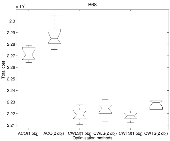
Figure 1: Boxplots of total costs for instances A32, A33, B45 and B68.

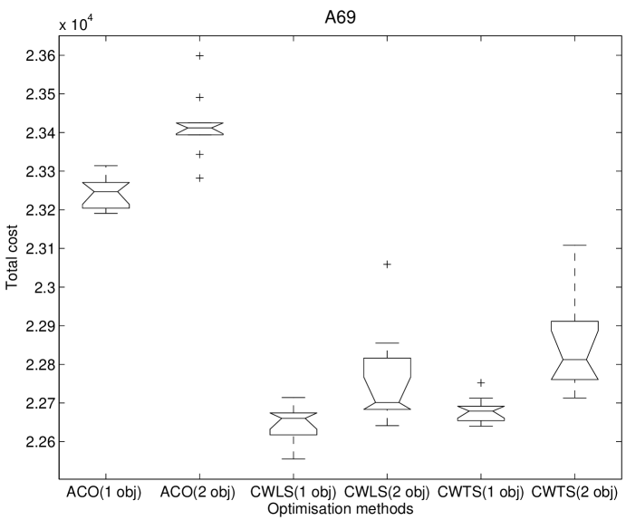
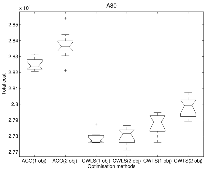
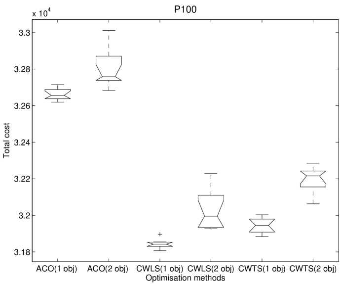
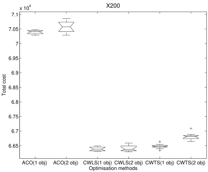
Figure 2: Boxplots of total costs for instances A69, A80, P100 and X200.

The boxplot consists of a box and whisker plot for each algorithm. The box has lines at the lower quartile, median, and upper quartile values. The whiskers are lines extending from each end of the box to show the extent of the rest of the data. Outliers are data with values beyond one standard deviation.

The conclusions that can be reached after analysis of the tests are as follows:

• The single objective approach yields the best performance in all instances.

• Considering separately the multi and single objective runs, in general there are no significant differences between CWLS and CWTS, although at first sight it would seem that CWLS performs better than CWTS on instances A32, A69, A80, P100 and X200 and vice versa on A33, B35, B45 and B67. On instance B68 there are no differences at first sight.

• ACO is significantly worse in all cases except B35. Furthermore, it is the method that scales worse, getting worse results as the size of the problem increases.

• The case of instance B35 is unique in the sense that monoobjective CWTS is significantly better than CWLS and does not differ significantly from ACO, both for single and multiobjective.

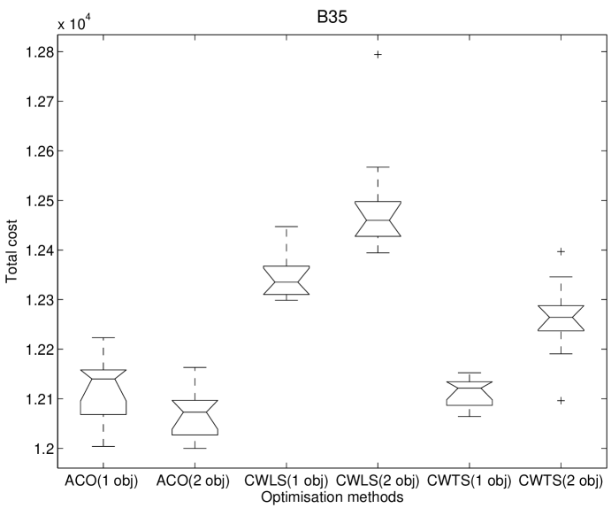
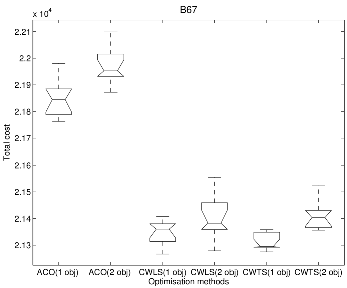
Figure 3: Boxplots of total costs for instances B35 and B67

In order to be able to compare results between the different instances we normalised the fitness values by defining the relative percentage deviation, $RPD$, given by the following expression:

$$RPD=\frac{fitness-fitness_{min}}{fitness_{min}}\times 100$$ (8)

where $fitness$ is the fitness value obtained by an algorithm configuration on a given instance. The $RPD$ is, therefore, the average percentage increase over the lower bound for each instance, $fitness_{min}$. In our case, the lower bound is the best result obtained for that instance across all algorithm configurations.

With the $RPD$ results of all the runs for all VRP solvers we ran the tests again; the results are shown in Figure 4 split into two groups: uniform distribution of shops and distribution in clusters. The conclusions in this case are similar. In both groups CWLS and CWTS perform better than ACO and, at first sight, CWLS is better than CWTS for group uniform and vice versa for group clusters. Further, considering each VRP solver separately, the single objective approach is better than the multiobjective one.

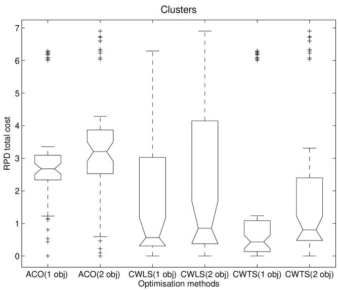
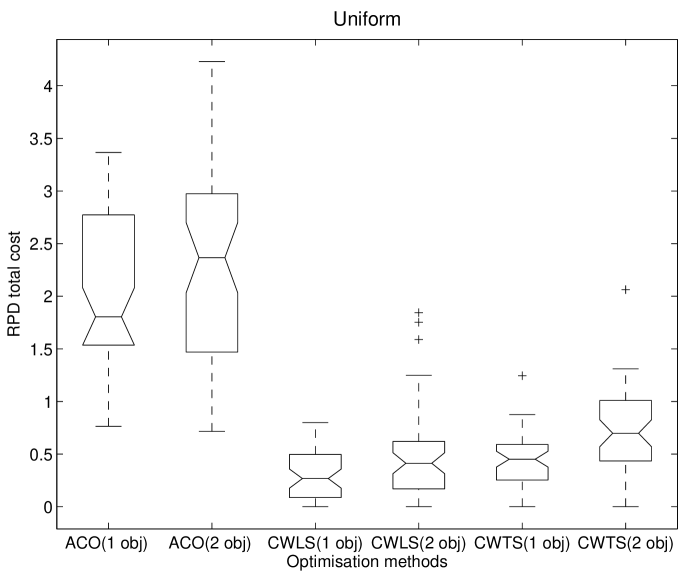
Figure 4: Boxplots of RPD of total costs for groups clusters (top) and uniform (bottom)

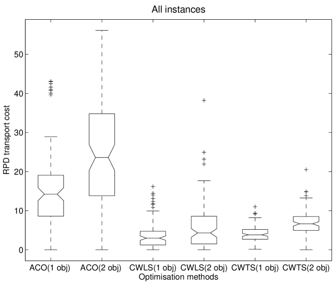
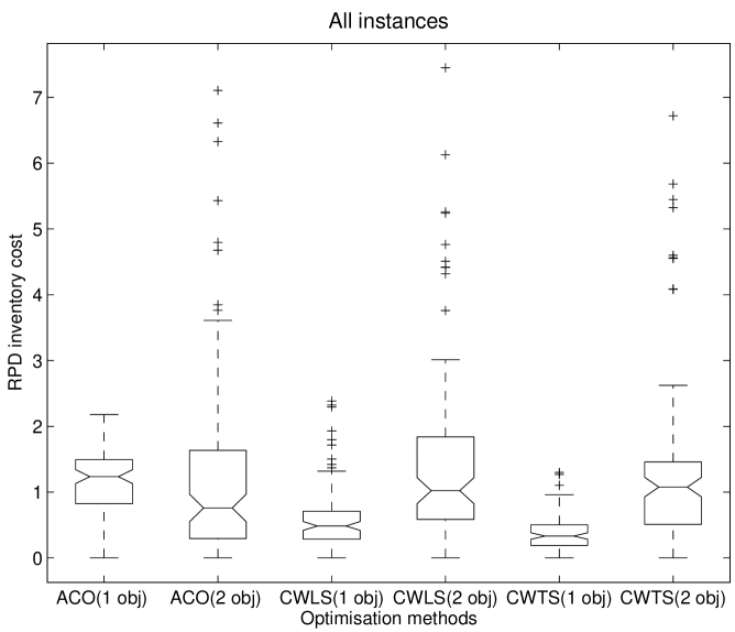
Figure 5: Boxplots for the transport (top) and inventory costs (bottom)

Figure 5 portrays the comparison between methods when the costs of transport and inventory are considered separately. Here it can be observed that there are no significant differences between methods if only inventory costs are taken into account. This differs from the conclusions obtained in (Esparcia-Alcázar et al., 2006a, ), where the choice of VRPsolver influenced the inventory cost results. In that work, however, the algorithms employed were suboptimal compared to the ones used here. So, it could be concluded that the choice of VRPsolver does not have an influence on the inventory costs provided a “good enough” algorithm is chosen.

The big difference lies in the transport costs, which is where ACO clearly shows its inferiority, especially in the multiobjective approach.

Regarding the computational time, the results clearly favour CWLS over all other VRP solvers. In general, when employing CWLS the time for a whole run took approximately the same as that of a single generation in when using CWTS or ACO. This is a point in favour of CWLS when considering a potential commercial application.

6.1 Pareto fronts

In this section we study the Pareto fronts obtained in the multiobjective approach in two instances of the problem, namely B35 and A32. The former has been chosen because of its uncharacteristic behaviour (as we have seen, in this instance ACO performs better than the other VRP solvers), and the latter because it is of a similar size. Pareto fronts for both instances are shown in Figure 6. In Table 8 we show the number of non-dominated solutions vs. the number of different individuals for each algorithm.

Table 8: Final population characteristics in multi-objective approach for one run of instances A32 and B35 using CWLS, ACO and CWTS as VRP-solvers. Population size is 100 individuals.

Instance A32
	No. of different individuals	Pareto front size	Ratio
CWLS	7	7	1
ACO	100	19	0.19
CWTS	24	24	1

Instance B35
	No. of different individuals	Pareto front size	Ratio
CWLS	18	18	1
ACO	100	8	0.08
CWTS	36	26	0.72

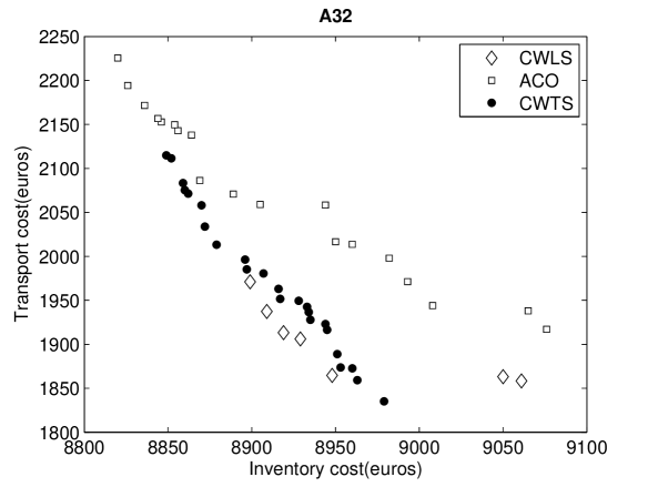
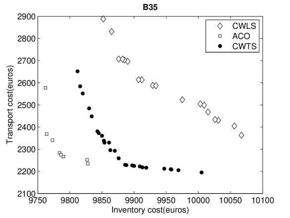
Figure 6: Pareto fronts in multi-objective approach for one run of instances A32 (left) and B35 (right) using CWLS, ACO and CWTS as VRP-solvers.

Comparing the number of non-dominated solutions in the final generation for each instance, we observe that the Pareto front yielded by the best performing VRP solver (CWLS in A32 and ACO in B35) has always a smaller size, whilst the one corresponding to the worst performing VRP solver has a bigger size (ACO in A32 and CWLS in B35). The figures also hint at the possibility that using CWLS or ACO as the VRP solver causes the Pareto front to converge to a very reduced set of solutions, while when using CWTS more non-dominated solutions are preserved.

On the other hand the ratio of repeated individuals over the population size is very high when using CWTS or CWLS, whilst in ACO there are no repeated individuals. It is possible that algorithm ACO has a slower rate of convergence than the other two in most of instances (except in cases such as B35), so it requires more generations to obtain equivalent results.

At this point it would be of interest to measure the quality of the Pareto front using one of the metrics that have been proposed for this purpose (Coello Coello,, 2005). However, many of them (e.g. the error ratio or the generational distance) assume that knowledge exists on the actual Pareto front, which is not the case here. Other metrics measure the distribution of solutions on the Pareto front by evaluating the variance of neighboring solutions. An example of this is the spacing, $SP$, which measures the relative distances between the members of Pareto front; a value of $SP=0$ means that members of the Pareto front are equispaced. The spacing is given by the following equation:

$$SP=\sqrt{\frac{1}{n-1}\sum_{i=1}^{n}\left(\overline{d}-d_{i}\right)^{2}}$$

where $n$ is the number of non-dominated solutions found, the distance $d_{i}$ is given by

$$d_{i}=min_{j}(|f_{1}^{i}(x)-f_{1}^{j}(x)|+|f_{2}^{i}(x)-f_{2}^{j}(x)|),\qquad i,j=1,...,n$$

where $f_{N}^{k}(\cdot)$ is the fitness of point $k$ on objective $N$, $x$ is the generation number and $\overline{d}$ is the mean of all $d_{i}$.

The values obtained are given in Table 9. From these we can see that the best values of the metric (i.e. the lowest spacing) are obtained by CWTS; however, from previous analysis we know that it is the other two VRP solvers that perform better: ACO for B35 and CWLS for A32. We can hence conclude that this metric is not very meaningful for the purposes of our problem.

Table 9: Values of the spacing for the Pareto fronts generated by all VRP solvers

	Problem instance
VRP solver	A32	B35
CWLS	17.605	23.937
ACO	12.823	68.027
CWTS	8.394	17.858

7 Conclusions and future work

We have shown how, for the problem presented here, the multiobjective approach does not yield any advantage over the single objective one. This could be explained by the fact that inventory costs are well above the transport costs. Given that the multiobjective approach does not prefer one objective over the other, it can happen that there are solutions for which transport costs are very low, but still that does not compensate for high inventory costs.

Further, we have shown how a classical algorithm such as Clarke and Wright’s, enhanced with local search, can be the best choice in the context of the Inventory and Transportation Problem, both in terms of the quality of the solutions obtained and the computational time necessary to achieve them. The power of other algorithms known to perform well in the context of VRP, such as ACO and TS, does not grant a good performance for the joint inventory and transportation problem. In general, using a global optimisation algorithm such as evolutionary computation jointly with a heuristic method adapted to the problem at hand, such as CWLS, yields the best results, so this is no surprise.

It could be argued that both TS and ACO require a finer tuning of their parameters in order to give an adequate performance than what was achieved here. This, however, could be interpreted as a disadvantage of their application to a variety of problem configurations and in a commercial context.

Special attention should be given to the case of instance B35, since it is the only one for which ACO yields better results than the remaining VRP solvers (with the exception of single objective TS) and, oddly, this happens in the multiobjective case. The geographical layout of this instance is shown in Figure 7; the high eccentricity of the distribution can be seen (the depot is on one side of the shops) compared to the small number of shops. Instance A80 also has a similar value of eccentricity, but for a higher number of shops. Perhaps here lies the explanation of why ACO works better in the former but not in the latter; clarifying this point is left for future work. In any case, we can conclude that although the CWLS with single objective approach performs better in general, it is nonetheless interesting to have a tool that can provide the possibility of using other VRP solvers and a multiobjective approach in order to handle special cases, such as B35.

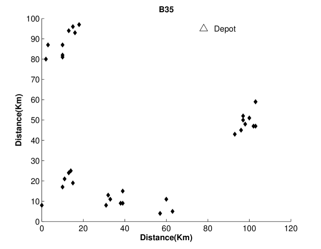
Figure 7: Geographical layout for instance B35

It must be noted that this result is subject to the specificities of the problem data, i.e. the fact that in this case the inventory cost greatly outweighs the cost of the transport. As future work we must consider a case in which the products moved are cheaper and hence the inventory cost is more in a par with the transport cost.

Appendix I: NSGA-II

NSGA-II (Deb et al.,, 2002, 2000) is an non-elitist multiobjective evolutionary algorithm (MOEA) which was developed in order to overcome the problems of previous MOEAs, such as the high computational complexity of sorting non dominated solutions. These algorithms have two common features: assigning fitness to population members based on nondominated sorting and preserving the diversity among solutions of the same nondominated front.

NSGA-II works as follows: Initially, a random parent population $P_{0}$ is created, with size N. The population is sorted based on nondominance. Each solution is assigned a fitness (or rank) equal to its nondomination level (with 1 being the best level). Initially, the usual binary tournament selection, recombination, and mutation operators are used to create an offspring population $Q_{0}$ of size N. For the remaining generations $t$ we do the following: First, a population $R_{t}$ of size 2N is formed as the union of $P_{t}$ and $Q_{t}$ and sorted according to nondomination in a number of fronts $F$. Next, a new population $P_{t+1}$ of size N is created by selecting individuals from $R_{t}$ in order of nondominance (i.e. ordered individuals from $F_{1}$ are chosen first, then ordered individuals from $F_{2}$ and so on until the number of individuals belonging to $P_{t+1}$ is N).

The advantages of NSGA-II with respect to previous MOEAs are the fast sorting of nondominated individuals and the preservation of diversity.

Nondominated sorting.

First, for each solution $p$ we calculate two entities: domination count, $n_{p}$, i.e. the number of solutions which dominate $p$, and a list of solutions that $p$ dominates, $S_{p}$. All solutions in the first nondominated front will have their $n_{p}$ as zero. Now, for each solution with $n_{p}=0$, we visit each member $q$ in its $S_{p}$ and reduce its domination count by one. In doing so, if for any member the domination count becomes zero, we place it in a separate list $Q$. These members belong to the second nondominated front. This procedure is continued with each member of $Q$ and the third front is identified. This process continues until all fronts are identified. The code for this operation can be found in Algorithm 2.

Procedure fastNonDominatedSort()

input: population $P$

output: listOfFronts $F$

For each $p\in P$

$S_{p}=\emptyset$

$n_{p}=0$

For each $q\in P$

if $p$ dominates $q$

Adds $q$ to $S_{p}$

else if $q$ dominates $p$

Increments $n_{p}$

if $n_{p}=0$

$p.rank=1$

Adds $p$ to $F_{1}$

$f=1$

while $F_{f}\not=\emptyset$

$Q=\emptyset$

for each $p\in F_{f}$

for each $q\in S_{p}$

Decrements $n_{q}$

if $n_{q}=0$

$q.rank=1$

Adds $q$ to $Q$

$F_{f}=Q$

Increments $f$

return $F$

end;

Algorithm 2 Nondominated sorting function for NSGAII.

Diversity preservation.

To get an estimate of the density of solutions surrounding a particular solution in the population, we calculate the average distance of two points on either side of this point along each of the objectives. This distance is called the crowding distance, and it is calculated as shown in Algorithm 3. Moreover, a crowded-comparison operator,$<_{n}$, is used in order to guide the selection process at the various stages of the algorithm towards a uniformly spread-out Pareto-optimal front.

In the selection process, given two solutions with different nondomination ranks the one with the lower (better) rank will be preferred. Otherwise, if both solutions belong to the same front, then one located in a less crowded region will be preferred.

Procedure crowdingDistance()

input: population pop[popSize]

for $i=1..popSize$

$pop[i].distance=0$

for each objective $m$

Sort $pop$ using $m$

$pop[1].distance=pop[popSize].distance=\infty$

for $i=2..popSize-1$

$pop[i].distance=pop[i].distance+(pop[i+1].m-pop[i-1].m)/(f_{m}^{max}-f_{m}^{min})$

end;

Algorithm 3 Crowding distance assignment for NSGA-II Algorithm.

For a complete description of NSGA-II, see (Deb et al.,, 2002, 2000).

Appendix II: Algorithms for solving the VRP

Here we describe the algorithms employed as VRPsolvers: C&W’s algorithm, Local Search, ACO and TS, plus other additional functions.

Algorithm CWLS

input: shops[nShops], depot

output: routes

[Build $nShops$ initial routes with one shop only]

for i=1… $nShops$

$r_{i}=(depot,shops[i],depot)$

[Calculate savings]

Calculate $s_{i,j}$ for each pair shops[i], shops[j]

$s_{i,j}=cost_{shops[i]depot}+cost_{depotshops[j]}-cost_{shops[i]shops[j]}$

[Best union ]

repeat

$s_{i*j*}=\max s_{i,j}$

Let $r_{i*}$ be the route containing shops[i]

Let $r_{j*}$ be the route containing shops[j]

if

shops[i*] is the last shop in $r_{i*}$

and shops[j*] is the first shop in $r_{j*}$

and the combination is feasible

then combine $r_{i*}$ and $r_{j*}$

delete $s_{i*j*}$;

until there are no more savings to consider;

return routes

end;

Algorithm 4 Clarke & Wright’s algorithm (C&W).

Algorithm LocalSearch

input: initialSolution

[Initialisation]

best $\leftarrow$ initialSolution

costBest = costTemp

[Improving each route]

for each r in routes(initialSolution)

for k=1..Max(sizeOf(r),numberOfNeighbors)

select s1, s2 random shops in r

tempSolution $\leftarrow$ InterchangeShops(initialSolution,s1, s2)

if (calculateCost(tempSolution) $<$ costBest)

best $\leftarrow$ tempSolution

costBest = calculateCost(best)

[Improving pairs of routes]

for r1 =1..routes(initialSolution)

for r2=r1+1..routes(initialSolution)

select s1 random shop in r1

select s2 random shop in r2

solTemp $\leftarrow$ InterchangeShops(initialSolution,s1, s2)

if (calculateCost(tempSolution) $<$ costBest)

best $\leftarrow$ tempSolution

costBest = calculateCost(best)

return best

end algorithm;

Algorithm 5 Local Search (LS) algorithm.

Algorithm ACO

input: shops[nShops], numberOfIterations

output: routes

[Initialise values]

routes $\leftarrow$ validRandomSolution

globalCost $\leftarrow$ calculateCost(routes)

[Main loop]

for it=1..numberOfIterations

[Looking for a solution for each ant]

for each ant i

Place ant i at depot

i.shopsNotVisited $\leftarrow$ shops

i.solution $\leftarrow\emptyset$

i.solution $\leftarrow$ reset cost, time and demand

reset load

while there are ants i for which i.shopsNotVisited $\neq\emptyset$ do

for each ant i for which i.shopsNotVisited $\neq\emptyset$

nextShopToVisit $\leftarrow$ TransitionFunction()

Update cost

if nextShopToVisit == depot then reset time and load

else

Update time, demand and load

Update i.shopsNotVisited, i.solution

Place ant i at nextShopToVisit

[Interchanges]

for each ant i do $\lambda$-interchanges in i.solution

[Update pheromone matrix with local solution]

Find worstPathInIteration, bestPathInIteration

Reinforce bestPathInIteration in pheromone matrix

Reset worstPathInIteration in pheromone matrix

[Update global solution]

if globalCost $>$ cost(bestPathInIteration)

routes $\leftarrow$ bestPathInIteration

globalCost $\leftarrow$ cost(bestPathInIteration)

[Update configuration]

Update algorithm parameters: $\rho$, p

return routes

end algorithm;

Algorithm 6 ACO - Main loop.

Algorithm Transition(shopsNotVisitedYet:List(shop),currentShop:shop,

remainingTime:float,remainingLoad:float):nextShop

$j=currentShop$

if ($q\leq p_{t}$)

$j=argmax_{shopsNotVisitedYet}[\tau_{currentShop,j}]^{\alpha}[\eta_{currentShop,j}]^{\beta}[\mu_{currentShop,j}]^{\gamma}$

else

$j=randomFrom(shopsNotVisitedYet)$

$time=TimeOf(currentShop,j)+TimeOf(j,Depot)$

if ($time\leq remainingTime$ AND $DemandOf(j)\leq remainingLoad$ )

nextShop = j

else

nextShop = Depot

return nextShop

end algorithm;

Algorithm 7 ACO - Transition function.

Algorithm TS

[Initialisation]

currentSolution $\leftarrow$ initialSolution

currentSolutionCost $\leftarrow$ calculateCost(currentSolution)

[Main loop]

while (iterations $<$ MAX-ITERATIONS)

bestNeighbour $\leftarrow$ getBestNeighbour (currentSolution, tabuList)

bestNeighbourCost $\leftarrow$ calculateCost(bestNeighbour)

currentSolution $\leftarrow$ bestNeighbour

currentSolutionCost $\leftarrow$ bestNeighbourCost

if (currentSolutionCost.isBetterThan(bestsolutionCost))

bestSolution $\leftarrow$ currentSolution

bestSolutionCost $\leftarrow$ currentSolutionCost

iterations $\leftarrow$ 0

else

iterations $\leftarrow$ iterations + 1

tabuList $\leftarrow$ updateTenure

return bestSolution

end algorithm;

Algorithm 8 Tabu Search (TS) algorithm - Main loop.

Algorithm bestNeighbour

[Initialisation]

moved $\leftarrow$ false

moves $\leftarrow$ getAllMoves

theBestNeighbour $\leftarrow$ currentSolution

theBestNeighbourCost $\leftarrow\infty$

neighbourCost $\leftarrow\infty$

[Main loop]

for i=1:moves.length

move $\leftarrow moves[i]$

neighbour $\leftarrow$ currentSolution

neighbour $\leftarrow$ move.operateOn(neighbour)

neighbourCost $\leftarrow$ calculateCost(neighbour)

isTabu $\leftarrow$ isTabu(move)

[Aspiration criteria]

if (neighbourCost $<$ bestSolutionCost)

isTabu $\leftarrow$ false

if (neighbourCost $<$ theBestNeighbourCost AND NOT isTabu)

theBestNeighbour $\leftarrow$ neighbour

theBestNeighbourCost $\leftarrow$ neighbourCost

bestNeighbourMove $\leftarrow$ move

moved $\leftarrow$ false

end for

[Update tabu list]

if moved == true

tabuList.addMove(bestNeighbourMove)

return theBestNeighbour

end algorithm;

Algorithm 9 Tabu Search - Best neighbour algorithm.

References

- Campbell and Savelsbergh, (2004) Campbell, A. and Savelsbergh, M. (2004). A decomposition approach for the Inventory-Routing Problem. Transportation Science, 38(4):488–502.
- Cardós and García-Sabater, (2006) Cardós, M. and García-Sabater, J. (2006). Designing a consumer products retail chain inventory replenishment policy with the consideration of transportation costs. International Journal of Production Economics, 104(2):525–535.
- Çetinkaya and Lee, (2000) Çetinkaya, S. and Lee, C. (2000). Stock replenishment and shipment scheduling for vendor-managed inventory systems. Management Science, 46(2):217–232.
- Clarke and Wright, (1964) Clarke, G. and Wright, W. (1964). Scheduling of vehicles from a central depot to a number of delivery points. Operations Research, 12:568–581.
- Coello Coello, (2005) Coello Coello, C. A. (2005). Evolutionary Multiobjective Optimization. Theoretical Advances and Applications. Springer.
- Coltorti and Rizzoli, (2007) Coltorti, D. and Rizzoli, A. E. (2007). Ant Colony Optimization for real-world vehicle routing problems. SIGEVOlution, 2(2):2–9.
- Cordeau et al., (1997) Cordeau, J.-F., Gendreau, M., and Laporte, G. (1997). A Tabu Search heuristic for periodic and multi-depot Vehicle Routing Problems. Networks, 30(2):105–119.
- Deb et al., (2000) Deb, K., Agrawal, S., Pratap, A., and Meyarivan, T. (2000). A fast elitist non-dominated sorting genetic algorithm for multi-objective optimisation: NSGA-II. In PPSN VI: Proceedings of the 6th International Conference on Parallel Problem Solving from Nature, pages 849–858, London, UK. Springer-Verlag.
- Deb et al., (2002) Deb, K., Pratap, A., Agarwal, S., and Meyarivan, T. (2002). A fast and elitist multiobjective genetic algorithm: NSGA-II. IEEE Transactions on Evolutionary Computation, 6(2):182–197.
- Dong and Xiang, (2006) Dong, L. W. and Xiang, C. T. (2006). Ant Colony Optimization for VRP and mail delivery problems. In IEEE International Conference on Industrial Informatics, pages 1143–1148. IEEE.
- Dorigo and Stutzle, (2004) Dorigo, M. and Stutzle, T. (2004). Ant Colony Optimization. MIT Press.
- dos Santos Coelho and Lopes, (2006) dos Santos Coelho, L. and Lopes, H. S. (2006). Supply chain optimization using chaotic differential evolution method. Systems, Man and Cybernetics, 2006. SMC ’06. IEEE International Conference on, 4:3114–3119.
- (13) Esparcia-Alcázar, A., Lluch-Revert, L., Cardós, M., Sharman, K., and Andrés-Romano, C. (2006a). A comparison of routing algorithms in a hybrid evolutionary tool for the Inventory and Transportation Problem. In Gary Yen, Lipo Wang, P. B. and Lucas, S., editors, Proceedings of the IEEE Congress on Evolutionary Computation, CEC 2006, pages 5605–5611, Vancouver, Canada. IEEE, Omnipress. ISBN: 0-7803-9489-5.
- (14) Esparcia-Alcázar, A., Lluch-Revert, L., Cardós, M., Sharman, K., and Andrés-Romano, C. (2006b). Design of a retail chain stocking up policy with a hybrid evolutionary algorithm. In Gottlieb, J. and Raidl, G., editors, EvoCOP 2006, volume LNCS 3906 of LNCS, pages 49–60. Springer. ISBN: 3-540-33178-6.
- (15) Esparcia-Alcázar, A., Lluch-Revert, L., Cardós, M., Sharman, K., and Merelo, J. (2007a). Configuring an evolutionary tool for the Inventory and Transportation Problem. In et al., M. K., editor, Proceedings of the Genetic and Evolutionary Computation Conference, GECCO 2007, volume II, pages 1975–1982, London, England. ACM Press.
- Esparcia-Alcázar et al., (2009) Esparcia-Alcázar, A. I., Cardós, M., Merelo, J., Martínez-García, A., García-Sánchez, P., Alfaro-Cid, E., and Sharman, K. (2009). EVITA: an integral evolutionary methodology for the Inventory and Transportation Problem. In Pereira, F. B. and Tavares, J., editors, Bio-Inspired Algorithms for the Vehicle Routing Problem, volume 161 of Studies in Computational Intelligence Series, pages 151–172. Springer. ISBN: 978-3-540-85151-6.
- (17) Esparcia-Alcázar, A. I., Lluch-Revert, L., Cardós, M., Sharman, K., and Andrés-Romano, C. (2007b). Configuración de una herramienta evolutiva para el problema de transporte e inventario. In Actas del V Congreso Español sobre Metaheurísticas, Algoritmos Evolutivos y Bioinspirados (MAEB’07), pages 1–8, Tenerife, Spain. ISBN: 978-84-690-3470-5.
- Federgruen and Zipkin, (1984) Federgruen, A. and Zipkin, P. (1984). Combined vehicle routing and inventory allocation problem. Operations Research, 32(5):1019–1037.
- Gendreau, (1999) Gendreau, M. (1999). An introduction to Tabu Search. In Glover, F. and Kochenberger, G., editors, Handbook of Metaheuristics, pages 37–54.
- Gendreau et al., (2002) Gendreau, M., Laporte, G., and Potvin, J. (2002). Methaheuristics for the Capacitated VRP. In Toth and Vigo, (2001), pages 144-145.
- Glover and Kochenberger, (2002) Glover, F. and Kochenberger, G. (2002). Handbook of Metaheuristics. Kluwer Academic Publishers.
- Martínez-García, (2008) Martínez-García, A. I. (2008). Resolución del VRP utilizando un algoritmo de hormigas. Informe Grupo Sistemas Adaptativos Complejos ITI-SAC-026, Instituto Tecnológico de Informática, Valencia, Spain. (in Spanish).
- Sindhuchao et al., (2005) Sindhuchao, S., Romeijn, H. E., Akçali, E., and Boondiskulchok, R. (2005). An integrated inventory-routing system for multi-item joint replenishment with limited vehicle capacity. J. of Global Optimization, 32(1):93–118.
- Toth and Vigo, (2001) Toth, P. and Vigo, D. (2001). The Vehicle Routing Problem. Society for Industrial and Applied Mathematics, Philadelphia, PA, USA. SIAM monography on Discrete Mathematics and Applications.
- Viswanathan and Mathur, (1997) Viswanathan, S. and Mathur, K. (1997). Integrating routing and inventory decisions in one-warehouse multiretailer multiproduct distribution systems. Manage. Sci., 43(3):294–312.
- Xiang-pei et al., (2006) Xiang-pei, H., Qiu-lei, D., Yong-xian, L., and Dan, S. (2006). An improved ant colony system and its application. In Computational Intelligence and Security, 2006 International Conference on, pages 384–389.
Acknowledgements
This work was part of project NoHNES - Non Hierarchical Network Evolutionary System, and has been supported by the Spanish Ministry of Science and Innovation, ref. TIN2007-68083-C02.