A Quintic Hypersurface in $\mathbb{P}^{8}(\mathbb{C})$ with Many Nodes

Abstract

We construct a hypersurface of degree $5$ in projective space $\mathbb{P}^{8}(\mathbb{C})$ which contains exactly 23436 ordinary nodes and no further singularities. This limits the maximum number $\mu_{8}(5)$ of ordinary nodes a hyperquintic in $\mathbb{P}^{8}(\mathbb{C})$ can have to $23436\leq\mu_{8}(5)\leq 27876$. Our method generalizes the approach by the $3^{\text{rd}}$ author for the construction of a quintic threefold with $130$ nodes in an earlier paper.

Introduction

Let $\mu_{n}(d)$ be the maximum number of ordinary nodes a hypersurface of degree $d$ in $\mathbb{P}^{n}:=\mathbb{P}^{n}(\mathbb{C})$ can have. It is known only for a few nontrivial cases: For curves in the plane we have $\mu_{2}(d)=d(d-1)/2$. In three–space, $\mu_{3}(d)$ is only known for $d\leq 6$; see [Bar, JR] for the case of degree six and [Lab] for an extensive overview. In $\mathbb{P}^{n}$ with $n\geq 4$, the best known upper bound is Varchenko’s spectral bound [Var]

$$\mu_{n}(d)\leq\operatorname{Ar}_{n}(d),$$

where $\operatorname{Ar}_{n}(d)$ is Arnold’s number:

$$\operatorname{Ar}_{n}(d):=\#\Big{\{}(k_{0},\ldots,k_{n})\in\big{(}(0,d)\cap\mathbb{Z}\big{)}^{n+1}\,\Big{|}\,\sum_{i=0}^{n}k_{i}=\Big{\lfloor}\frac{nd}{2}\Big{\rfloor}+1\Big{\}}.$$

All currently best known lower bounds follow from symmetric constructions: Kalker [Kal] constructed $\Sigma_{n}$-symmetric cubics which show $\mu_{n}(3)=\operatorname{Ar}_{n}(3)={n+1\choose\lfloor\frac{n}{2}\rfloor}$ for any $n$. Goryunov constructed $A_{n+1}$- and $B_{n+1}$-symmetric quartics in $\mathbb{P}^{n}$, which reach approximately $86\%$ of the Arnold-Varchenko upper bound (cf. [Gor]). In [vStr], a $\Sigma_{6}$-symmetric quintic in $\mathbb{P}^{4}$ with $130$ nodes was constructed which limits the possibilities for $\mu_{4}(5)$ to $130\leq\mu_{4}(5)\leq 135=\operatorname{Ar}_{4}(5).$

In sections 1 to 3, we consider the case of $\Sigma_{n+2}$-invariant quintics and construct an example in $\mathbb{P}^{8}$ with $23436$ nodes which yields

$$23436\leq\mu_{8}(5)\leq 27876=\operatorname{Ar}_{8}(5).$$

For most other $n$, it seems that a pentagon–symmetric construction yields more nodes than our approach; we discuss this briefly in section 4.

1 $\Sigma_{n+2}$-symmetric Hyperquintics

Adapting the approach used in [vStr], we consider the 1-parameter-family of $\Sigma_{n+2}$-symmetric hyperquintics $Q:=Q_{(\alpha:\beta)}$ given by

$$F_{(\alpha:\beta)}:=\alpha S_{5}+\beta S_{2}S_{3}=0\,,\quad(\alpha:\beta)\in\mathbb{P}^{1}\,,$$

in projective space $\mathbb{P}^{n}(\mathbb{C})$, which is defined by $S_{1}=0$ in $\mathbb{P}^{n+1}(\mathbb{C})$. Here, $S_{i}$ denotes the $i$-th elementary-symmetric polynomial in the space coordinates of $\mathbb{P}^{n+1}$:

$$S_{i}=\sum_{0\leq j_{1}<\ldots<j_{i}\leq n+1}x_{j_{1}}\cdot\ldots\cdot x_{j_{i}},\qquad i=1,\ldots,5\,.$$

To determine the singular locus of each quintic in the pencil, it turns out to be convenient to rewrite $F_{(\alpha:\beta)}$ in terms of the $i$-th power sums in the coordinates $x_{j}$ defined by

$$C_{i}:=\sum^{n+1}_{j=0}x_{j}^{i},\qquad i=1,\ldots,5.$$

Modulo $S_{1}$, we have the following identities:

$$S_{1} =C_{1},$$

$$S_{2} =\textstyle-\frac{1}{2}C_{2},$$

$$S_{3} =\textstyle\frac{1}{3}C_{3},$$

$$S_{4} =\textstyle-\frac{1}{4}C_{4}+\frac{1}{8}C_{2}^{2},$$

$$S_{5} =\textstyle\frac{1}{5}C_{5}-\frac{1}{6}C_{2}C_{3}.$$

So the hyperquintic $Q=Q_{(\alpha:\beta)}$ is given by

$$F_{(\alpha:\beta)}=\alpha S_{5}+\beta S_{2}S_{3}=\textstyle\frac{\alpha}{5}C_{5}-\frac{\alpha+\beta}{6}C_{2}C_{3}=0\,.$$

Since $F_{(0:1)}=-\frac{1}{6}C_{2}C_{3}=S_{2}S_{3}$ clearly has the projective variety $S_{2}=S_{3}=0$ as singular locus, we assume $\alpha\not=0$. The singular points of the hyperquintics are those where the gradients of the defining equations in $\mathbb{P}^{n+1}$ are dependent. So we have

$$\eta\text{ singular}\qquad \Leftrightarrow\qquad\operatorname{rank}\left(\begin{array}[]{ccc}\partial_{0}F_{(\alpha:\beta)}(\eta)&\ldots&\partial_{n+1}F_{(\alpha:\beta)}(\eta)\\ \partial_{0}S_{1}(\eta)&\ldots&\partial_{n+1}S_{1}(\eta)\\ \end{array}\right)\leq 1$$

$$\Leftrightarrow\qquad\operatorname{rank}\left(\begin{array}[]{ccc}\partial_{0}F_{(\alpha:\beta)}(\eta)&\ldots&\partial_{n+1}F_{(\alpha:\beta)}(\eta)\\ 1&\ldots&1\\ \end{array}\right)\leq 1$$

$$\Leftrightarrow\qquad\exists\,\mu\in\mathbb{C}:\partial_{i}F_{(\alpha:\beta)}(\eta)=\mu\,,\qquad i=0,\ldots,n+1\,.$$

Hence, for all indices $i=0,\ldots,n+1$ we obtain

$$\sum_{j=0}^{n+1}\partial_{j}F_{(\alpha:\beta)}(\eta)=(n+2)\cdot\mu=(n+2)\cdot\partial_{i}F_{(\alpha:\beta)}(\eta),$$

which leads via $S_{1}=0$ to the following lemma.

Lemma 1

Each coordinate $\eta_{i}$ of a singularity $\eta$ of the hyperquintic $Q_{(\alpha:\beta)}$ in $\mathbb{P}^{n}=V(S_{1}(x_{0},\ldots,x_{n+1}))$ is a root of

$$P(X):=P_{\lambda}(X):=\textstyle X^{4}-X^{2}\cdot\lambda C_{2}-X\cdot\frac{2}{3}\lambda C_{3}+\frac{1}{n+2}\big{(}\lambda C_{2}^{2}-C_{4}\big{)}=0,$$

where $\lambda:=\frac{\alpha+\beta}{2\alpha}$.

$\square$

Note that the sum of the four roots of $P(X)$ is zero since the term $X^{3}$ does not occur.

2 The Family of $\Sigma_{10}$-symmetric Hyperquintics in $\mathbb{P}^{8}$

We now specialize to the case $n=8$. According to Lemma 1, each coordinate $\eta_{i}$ of a singularity $\eta$ of the hyperquintic $Q_{(\alpha:\beta)}$ in $\mathbb{P}^{8}$ satisfies

$$P(X)=\textstyle X^{4}-X^{2}\cdot\lambda C_{2}-X\cdot\frac{2}{3}\lambda C_{3}+\frac{1}{10}\big{(}\lambda C_{2}^{2}-C_{4}\big{)}=0\,,$$

where $\lambda=\frac{\alpha+\beta}{2\alpha}$. A priori, there are 23 cases to check, since the 10 coordinates may be distributed over the four roots $a,b,c,d$ of $P$ as follows:

Case 1:	$10a$	Case 9:	$6a,3b,c$	Case 17:	$4a,4b,2c$
Case 2:	$9a,b$	Case 10:	$6a,2b,2c$	Case 18:	$4a,4b,c,d$
Case 3:	$8a,2b$	Case 11:	$6a,2b,c,d$	Case 19:	$4a,3b,3c$
Case 4:	$8a,b,c$	Case 12:	$5a,5b$	Case 20:	$4a,3b,2c,d$
Case 5:	$7a,3b$	Case 13:	$5a,4b,c$	Case 21:	$4a,2b,2c,2d$
Case 6:	$7a,2b,c$	Case 14:	$5a,3b,2c$	Case 22:	$3a,3b,3c,d$
Case 7:	$7a,b,c,d$	Case 15:	$5a,3b,c,d$	Case 23:	$3a,3b,2c,2d$
Case 8:	$6a,4b$	Case 16:	$5a,2b,2c,d$

We analyse some example cases here; the remaining cases can be found in the appendix. First, we determine only the $\Sigma_{10}$-orbit length of the corresponding singularity $\eta$. Then, we further check for nodes in those cases that produced the longest orbits under $\Sigma_{10}$.

Case 1

does not occur, since on the one hand $\eta=(x:\ldots:x)\in\mathbb{P}^{8}$, and on the other hand the sum of its coordinates has to be zero.

Case 2

Assume that $\eta=(1:1:1:1:1:1:1:1:1:-9)$. Hence $C_{2}=90$, $C_{3}=-720$, $C_{4}=6570$, and

$$P(X)=\textstyle X^{4}-90\lambda X^{2}+480\lambda X+810\lambda-657\,.$$

Requiring $P(1)=P(-9)=0$, we obtain $\lambda=\frac{41}{75}$, thus

$$(\alpha:\beta)=(75:7)\,.$$

The length of the $\Sigma_{10}$-orbit of $\eta$ is 10.

Case 7

A priori, we have $\eta=(a:a:a:a:a:a:a:b:c:d)$. Since $7a+b+c+d=0$ and $a+b+c+d=0$, we obtain $a=0=b+c+d$ and $\eta=(0:0:0:0:0:0:0:b:c:-b-c)$. Since $b=c=0$ is impossible, w.l.o.g. we put $b=1$. By $P(0)=P(1)=P(c)=P(-1-c)=0$ we have $2\lambda=1$, hence

$$(\alpha:\beta)=(1:0),$$

and no further conditions on $c\in\mathbb{C}$ . Thus, we have found $120=\frac{10\cdot 9\cdot 8}{3!}$ singular lines.

Case 12

We have $\eta=(1:1:1:1:1:-1:-1:-1:-1:-1)$ and, thus, $C_{2}=C_{4}=10$, $C_{3}=0$, and

$$P(X)=X^{4}-10\lambda X^{2}+10\lambda-1=\big{(}X^{4}-1\big{)}-10\lambda\big{(}X^{2}-1\big{)}\,.$$

Hence, $P(\pm 1)=0$ holds for all $\lambda$. This means that every single point in the $\Sigma_{10}$-orbit of $\eta$ is a singularity of each hyperquintic $Q=Q_{(\alpha:\beta)}$ in the $\Sigma_{10}$-symmetric family in $\mathbb{P}^{8}$. For this reason, from now on we will call these points generic singularities (cf. [Schm]). The length of the $\Sigma_{10}$-orbit of $\eta$ is $126=\frac{1}{2}\cdot{10\choose 5}$.

Case 18

Due to $4a+4b+c+d=a+b+c+d=0$ we immediately obtain $b=-a$ and $d=-c$, hence $\eta=(a:a:a:a:-a:-a:-a:-a:c:-c)$. Since $a=0$ leads us back to case 4, we put $a=1$ and find $C_{2}=2c^{2}+8$, $C_{3}=0$, $C_{4}=2c^{4}+8$, and $P$ appropriate. Via $P(\pm 1)=P(\pm c)=0$ we obtain

$$0=\big{(}2\lambda(c^{2}+4)-(c^{2}+1)\big{)}(c+1)(c-1)\,.$$

With $c=\pm 1$ we are back in case 12, so we assume $c\not=\pm 1$. Thus,

$$0=(2\lambda-1)c^{2}+(8\lambda-1)\,.$$

This equation has no solution for $\lambda=\frac{1}{2}$, but for $\lambda\not=\frac{1}{2}$ we have

$$0=\beta c^{2}+(3\alpha+4\beta)\,. \hskip 85.35826pt(*)$$

Thus, $\eta=(1:1:1:1:-1:-1:-1:-1:c:-c)$ is a singular point of $Q_{(\alpha:\beta)}$ , $(\alpha:\beta)\not=(1:0)$ , for all $c\in\mathbb{C}$  that satisfy $(*)$.

There are $3150=\frac{1}{2}\cdot{10\choose 4}{6\choose 4}$ elements in the $\Sigma_{10}$-orbit of $\eta$, which we will also call generic singularities as well as in case 12 (cf. [Schm]).

If $(\alpha:\beta)\in\{\,(5:-3),(4:-3)\,\}$ , which means $\lambda\in\{\,\frac{1}{5},\frac{1}{8}\,\}$, the solutions of $(*)$ are $c=\pm 1$ and $c=0$, respectively, so $\eta$ coincides with the singular points from case 12 or two orbit elements of $\eta$ merge to one of the singularities from case 17. Hence, we have singularities that are worse than ordinary nodes. A proof of this is given in section 3. For this reason, we from now on will refer to $(\alpha:\beta)\in\{\,(1:0),(5:-3),(4:-3)\,\}$  or $\lambda\in\{\,\frac{1}{2},\frac{1}{5},\frac{1}{8}\,\}$ as exceptional values. Case 7, however, already showed that $Q_{(1:0)}$ contains 120 singular lines.

We list the results of our investigation below. Table 1 shows the generic singularities, which are contained in each hyperquintic of the family. For the exceptional values $(\alpha:\beta)\in\left\{(1:0),(2:-1),(3:-2),(4:-3),(5:-3)\right\}$, the corresponding hyperquintics have singularities worse than ordinary nodes.

In table 2 we list the parameter values, for which we have additional orbits of singular points. Using computer algebra we can verify that all the additional orbits consist only of ordinary nodes, if not stated otherwise.

orbit length	orbit element	case
126	$(1:1:1:1:1:-1:-1:-1:-1:-1)$	12
	$(1:1:1:1:-1:-1:-1:-1:c:-c)$ ,
3150	$\beta c^{2}+(3\alpha+4\beta)=0$	18
	$(1:1:1:-1:-1:-1:c:c:-c:-c)$ ,
12600	$(\alpha+2\beta)c^{2}+(2\alpha+3\beta)=0$	23

Table 1: Generic singularities in $\mathbb{P}^{8}$. Each hyperquintic $Q_{(\alpha:\beta)}$ of the 1-parameter-family in $\mathbb{P}^{8}$ with $(\alpha:\beta)$ not an exceptional value contains these singular points.

$(\alpha:\beta)$	orbit length	orbit element
		$(1:1:1:1:1:b_{1}:b_{1}:b_{2}:b_{2}:3)$ ,
$(3:-1)$	7560	$b_{1,2}=-2\pm\sqrt{-3}$
		$(3:3:3:3:b_{1}:b_{1}:b_{1}:b_{2}:b_{2}:b_{2})$ ,
$(7:-5)$	4200	$b_{1,2}=-2\pm\sqrt{-3}$
		$(1:1:1:1:1:1:-5:-5:c_{1}:c_{2})$ ,
$(51:-25)$	2520	$c_{1,2}=2\pm\sqrt{-7/5}$
		$(2\!:\!2\!:\!2\!:\!2\!:\!2\!:\!2b\!:\!2b\!:\!2b\!:\!-5\!-\!3b\!:\!-5\!-\!3b)$
$(280\!:\!-163\pm\!3\sqrt{65})$	2520	$b=\frac{3\pm\sqrt{65}}{2}$
		$(1:1:1:1:1:b:b:b:b:-4b-5)$ ,
$(30:-13\mp\sqrt{85})$	1260	$b=\frac{-29\pm\sqrt{85}}{14}$
		$(1:1:1:1:1:1:b_{1}:b_{1}:b_{2}:b_{2})$ ,
$(4:-1)$	1260	$b_{1,2}=\frac{-3\pm\sqrt{-7}}{2}$
		$(1:1:1:1:1:1:b:b:b:-3b-6)$ ,
​$(21\!:\!2b^{3}\!+\!25b^{2}\!+\!86b\!+\!76)$​	840	$2b^{4}+25b^{3}+93b^{2}+139b+77=0$
		$(1:1:1:1:1:1:1:b:b:-2b-7)$ ,
​$(84\!:\!175\!-\!3b(b^{2}\!+\!5b\!-\!13))$​	360	$3b^{4}+39b^{3}+189b^{2}+413b+364=0$
$(50:-37)$	210	$(2:2:2:2:2:2:-3:-3:-3:-3)$
$(175:-117)$	120	$(3:3:3:3:3:3:3:-7:-7:-7)$
		$(1:1:1:1:1:1:1:1:b_{1}:b_{2})$ ,
$(3:7)$	90	$b_{1,2}=-4\pm\sqrt{-11}$
$(100:-49)$	45	$(1:1:1:1:1:1:1:1:-4:-4)$
$(75:7)$	10	$(1:1:1:1:1:1:1:1:1:-9)$
		$(0:0:0:0:0:0:0:b:c:d)$ ,
$(1:0)$	120 lines	$b+c+d=0$
		$(0:0:0:0:b:b:c:c:d:d)$ ,
$(2:-1)$	3150 lines	$b+c+d=0$
		$(a:a:a:b:b:b:c:c:c:0)$ ,
$(3:-2)$	2800 lines	$a+b+c=0$
	1575 ($D_{4}$)
$(4:-3)$	(Remark 2)	$(1:1:1:1:-1:-1:-1:-1:0:0)$
	126
$(5:-3)$	(Remark 1)	$(1:1:1:1:1:-1:-1:-1:-1:-1)$
	hypersurface
$(0:1)$	$S_{2}=S_{3}=0$

Table 2: Parameter values, for which we have additional orbits of singular points. By using computer algebra we can verify that only ordinary nodes are contained in these orbits, if not stated otherwise.

As we will see in the next section, all the generic singularities are ordinary nodes. Moreover, for $(\alpha:\beta)=(3:-1)$, which corresponds to the longest orbit of additional singular points, we find the best hyperquintic in the $\Sigma_{10}$-symmetric family in $\mathbb{P}^{8}$.

Theorem 1

The hyperquintic $Q_{(3:-1)}$, given by

$$3\cdot S_{5}+(-1)\cdot S_{2}S_{3}\,=\,S_{1}\,=\,0,$$

where $S_{i},\;i=1,2,3,5,$ is the $i$-th elementary-symmetric polynomial in 10 variables, has exactly 23436 ordinary nodes and no further singularities.

$\square$

3 Ordinary Nodes

To show that all the isolated singularities are ordinary nodes, we use the Hessian criterion, i.e. we show $\det(\operatorname{Hess}_{f}(y))\not=0$, where $\operatorname{Hess}_{f}=\left(\frac{\partial^{2}f}{\partial x_{i}\partial x_{j}}\right)_{\!ij}$ is the Hessian of $f$, $f=0$ is the affine equation of the hyperquintic $Q_{(\alpha:\beta)}$ in an appropriate affine chart, and $y$ is the singular point in this chart.

Modulo $S_{1}$ one has

$$F:= \,\textstyle F_{(1:\beta)}=S_{5}+\beta\cdot S_{2}S_{3}=\frac{1}{5}C_{5}-\frac{1+\beta}{6}C_{2}C_{3}$$

$$= \,\frac{1}{5}\bigg{(}\sum_{i=0}^{8}x_{i}^{5}-g(x)^{5}\bigg{)}-\frac{1+\beta}{6}\bigg{(}\sum_{i=0}^{8}x_{i}^{2}+g(x)^{2}\bigg{)}\bigg{(}\sum_{i=0}^{8}x_{i}^{3}-g(x)^{3}\bigg{)},$$

where $g(x):=x_{0}+\ldots+x_{8}$. We consider the isolated singularities in affine charts $\mathbb{A}^{8}_{\,i}$, $i\in\{\,0,\ldots,8\,\}$, given by

$$\mathbb{A}^{8}_{\,i}:=\big{\{}(x_{0},\ldots,x_{i-1},x_{i+1},\ldots,x_{8})| (x_{0}:\ldots:x_{i-1}:1:x_{i+1}:\ldots:x_{9})\in\mathbb{P}^{8},$$

$$\hskip 2.84526pt\,x_{9}=-(x_{0}+\ldots+x_{8})\,\big{\}}.$$

Those charts cover the projective space $\mathbb{P}^{8}$, so that we find all the isolated singularities in at least one chart $\mathbb{A}^{8}_{\,i}$. In our case it is even sufficient to check only one chart, w.l.o.g. $\mathbb{A}^{8}:=\mathbb{A}^{8}_{\,0}$, since no coordinate of our isolated singularities is zero. Defining $h(x):=1+x_{1}+\ldots+x_{8}$, we obtain

$$f:= f(x_{1},\ldots,x_{8}):=\,F\big{(}1,x_{1},\ldots,x_{8},-(1+x_{1}+\ldots+x_{8})\big{)}$$

$$= \,\frac{1}{5}\bigg{(}1+\sum_{k=1}^{8}x_{k}^{5}-h(x)^{5}\bigg{)}-\frac{1+\beta}{6}\bigg{(}1+\sum_{k=1}^{8}x_{k}^{2}+h(x)^{2}\bigg{)}\bigg{(}1+\sum_{k=1}^{8}x_{k}^{3}-h(x)^{3}\bigg{)}.$$

Thus, it holds for the partial derivatives $f_{i}=\frac{\partial f}{\partial x_{i}}$, $i=1,\ldots,8$, of $f$

$$f_{i} =x_{i}^{4}-h(x)^{4}{\textstyle-\frac{1+\beta}{6}\bigg{[}2(x_{i}+h(x))+3(x_{i}^{2}-h(x)^{2})}+2\cdot\sum_{k=1}^{8}x_{k}^{3}(x_{i}+h(x))$$

$$\hskip 85.35826pt+3\cdot\sum_{k=1}^{8}x_{k}^{2}(x_{i}^{2}-h(x)^{2})-2x_{i}h(x)^{3}+3x_{i}^{2}h(x)^{2}-5h(x)^{4}\bigg{]}$$

and for the second partial derivatives $f_{ii}=\frac{\partial^{2}f}{\partial x_{i}^{2}}$ and $f_{ij}=\frac{\partial^{2}f}{\partial x_{i}\partial x_{j}}$, $i\not=j$,

$$f_{ii} =4x_{i}^{3}-4h(x)^{3}{\textstyle-\frac{1+\beta}{6}}\bigg{[}4+6x_{i}-6h(x)+12x_{i}^{3}+12x_{i}^{2}h(x)+4\cdot\sum_{k=1}^{8}x_{k}^{3}$$

$$\hskip 125.19194pt-6x_{i}h(x)^{2}+6(x_{i}-h(x))\sum_{k=1}^{8}x_{k}^{2}-22h(x)^{3}\bigg{]},$$

$$f_{ij} =-4h(x)^{3}\textstyle-\frac{1+\beta}{6}\bigg{[}2-6h(x)+6x_{i}x_{j}(x_{i}+x_{j})+6h(x)(x_{i}^{2}+x_{j}^{2})$$

$$\hskip 62.59596pt-6h(x)^{2}(x_{i}+x_{j})+2\cdot\sum_{k=1}^{8}x_{k}^{3}-6h(x)\cdot\sum_{k=1}^{8}x_{k}^{2}-20h(x)^{3}\bigg{]}.$$

In the following subsections, we first check that all generic singularities are ordinary nodes. Then we verify that the longest orbit of length 7560 of the additional singularities of $Q_{(3:-1)}$ consists only of ordinary nodes.

3.1 The 126 generic Nodes

We consider $\eta:=(1:1:1:1:1:-1:-1:-1:-1:-1)$ with its 126 orbit elements; due to our choice of the affine chart $\mathbb{A}^{8}$ and $S_{1}=0$, we evaluate the Hessian $\operatorname{Hess}_{f}=\big{(}f_{ij}\big{)}$ in $y:=(1,1,1,1,-1,-1,-1,-1)$. With $h(y)=1$, we obtain

$$f_{ii}(y)=\left\{\begin{array}[]{r@{,\;}l}0&\text{ if }i\leq 4,\\ 12+20\beta&\text{ if }i>4,\end{array}\right. f_{ij}(y)=6+10\beta\text{ for all }i\not=j.$$ and

Thus,

$$\operatorname{Hess}_{f}(y)=\big{(}6+10\beta\big{)}\cdot\left(\begin{array}[]{cccccccc}0&1&\cdots&\cdots&\cdots&\cdots&\cdots&1\\ 1&0&\ddots&&&&&\vdots\\ \vdots&\ddots&0&\ddots&&1&&\vdots\\ \vdots&&\ddots&0&\ddots&&&\vdots\\ \vdots&&&\ddots&2&\ddots&&\vdots\\ \vdots&&1&&\ddots&2&\ddots&\vdots\\ \vdots&&&&&\ddots&2&1\\ 1&\cdots&\cdots&\cdots&\cdots&\cdots&1&2\\ \end{array}\right).$$

The determinant of the righthand matrix is 1, hence

$$\det(\operatorname{Hess}_{f}(y))\not=0\;\text{ for all }\textstyle\beta\not=-\frac{3}{5}.$$

But $(\alpha:\beta)=(1:-\frac{3}{5})=(5:-3)$ is one of the exceptional values, hence all of the 126 orbit elements of $\eta$ are ordinary nodes of $Q_{(\alpha:\beta)}$, $(\alpha:\beta)\not=(5:-3)$, $\alpha\not=0$. For $(\alpha:\beta)=(5:-3)$ we have singularities worse than ordinary nodes.

3.2 The 3150 generic Nodes

Now consider $\eta:=(1:1:1:1:-1:-1:-1:c:-c:-1)$ and its orbit elements, where $\beta c^{2}+(3+4\beta)=0$, in the affine chart $\mathbb{A}^{8}$. We put $y:=(1,1,1,-1,-1,-1,c,-c)$ and obtain

$$h(y)=(1+y_{1}+\ldots+y_{8})=1,\quad \quad\sum_{k=1}^{8}y_{k}^{3}=0,\quad \sum_{k=1}^{8}y_{k}^{2}=6+2c^{2}.$$

Let

$$b_{1}:= \,-4+(1+\beta)(8+2c^{2})\,,$$

$$b_{4}:= \;6+10\beta\,,$$

$$b_{5}:= \;4c^{3}-4-(1+\beta)(4c^{3}+6c-10)\,,$$

$$b_{6}:= \,-4c^{3}-4+(1+\beta)(4c^{3}+6c+10)\,,$$

then we have

$f_{11}(y)=f_{22}(y)=f_{33}(y)=0,$	$f_{44}(y)=f_{55}(y)=f_{66}(y)=2b_{1},$
$f_{77}(y)=b_{5},$	$f_{88}(y)=b_{6}$,

and for $i\not=j$

$$f_{ij}(y)=\left\{\begin{array}[]{r@{,\quad}l}b_{1}&y_{i}=y_{j}=+1,\\ b_{1}&y_{i}=y_{j}=-1,\\ b_{1}&y_{i}=+1,\;y_{j}=-1,\\ b_{4}&y_{i}=+1,\;y_{j}=+a,\\ b_{4}&y_{i}=+1,\;y_{j}=-a,\\ b_{1}&y_{i}=-1,\;y_{j}=+a,\\ b_{1}&y_{i}=-1,\;y_{j}=-a,\\ b_{4}&y_{i}=+a,\;y_{j}=-a.\end{array}\right.$$

Hence, for the Hessian $\operatorname{Hess}_{f}(y)$ we have

$$\operatorname{Hess}_{f}(y)=\left(\begin{array}[]{ccc|ccc|c|c}0&b_{1}&b_{1}&b_{1}&b_{1}&b_{1}&b_{4}&b_{4}\\ b_{1}&0&b_{1}&b_{1}&b_{1}&b_{1}&b_{4}&b_{4}\\ b_{1}&b_{1}&0&b_{1}&b_{1}&b_{1}&b_{4}&b_{4}\\ \hline\cr b_{1}&b_{1}&b_{1}&2b_{1}&b_{1}&b_{1}&b_{1}&b_{1}\\ b_{1}&b_{1}&b_{1}&b_{1}&2b_{1}&b_{1}&b_{1}&b_{1}\\ b_{1}&b_{1}&b_{1}&b_{1}&b_{1}&2b_{1}&b_{1}&b_{1}\\ \hline\cr b_{4}&b_{4}&b_{4}&b_{1}&b_{1}&b_{1}&b_{5}&b_{4}\\ \hline\cr b_{4}&b_{4}&b_{4}&b_{1}&b_{1}&b_{1}&b_{4}&b_{6}\\ \end{array}\right).$$

Performing row and column transformations, one easily finds

$$\det(\operatorname{Hess}_{f}(y))=2^{8}\cdot c^{2}\cdot(c^{2}-1)^{8}\cdot\frac{3^{2}}{(c^{2}+4)^{2}}\,.$$

The denominator is not zero, since this would lead to a contradiction with the constraint on $c$. So the determinant only vanishes for $c\in\{0,\pm 1\}$. But $c$ takes these values only for $(\alpha:\beta)\in\{(5:-3),(4:-3)\}$, which are exceptional values. Then we have singularities worse than ordinary nodes, due to certain merging singularities. For other values of $(\alpha:\beta)$, $\alpha\not=0$, all the 3150 orbit elements of $\eta$ are ordinary nodes.

3.3 The 12600 generic and the 7560 additional Nodes

For the 12600 orbit elements of $(1:1:1:-1:-1:-1:c:c:-c:-c)$ with $(1+2\beta)\cdot c^{2}+(2+3\beta)=0$ as well as for the 7560 additional orbit elements of $(1:1:1:1:1:b_{1}:b_{1}:b_{2}:b_{2}:3)$ with $b_{1,2}=-2\pm\sqrt{-3}$, the procedure is exactly the same. For the latter case, we take $\beta=-\frac{1}{3}$ into account, since it is an additional orbit of singularities for $Q_{(3:-1)}=Q_{(1:-\frac{1}{3})}$. Thus, we find $\det(\operatorname{Hess}_{f}(y_{1}))\not=0$ for $(\alpha:\beta)\not=(5:-3),(3:-2)$, and $\det(\operatorname{Hess}_{f}(y_{2}))\not=0$, where $y_{1}:=(1,1,-1,-1,c,c,-c,-c)$ and $y_{2}:=(1,1,1,1,b_{1},b_{1},b_{2},b_{2})$. So the 12600 generic and the 7560 additional orbit elements of the corresponding singularities are ordinary nodes. The latter ones are contained only in $Q_{(3:-1)}$.

4 Concluding Remarks

We have proved in the previous sections that the hyperquintic $Q_{(3:-1)}$ in $\mathbb{P}^{8}$ has 23436 ordinary nodes and no further singularities. We now briefly discuss the cases $(\alpha:\beta)$, where $Q_{(\alpha:\beta)}$ has higher singularities (see table 2). Moreover, we look at the generalization of our approach to $\mathbb{P}^{n}$ and compare it to another construction of hyperquintics in $\mathbb{P}^{n}$ with many nodes.

4.1 Some Cases with higher Singularities

Remark 1

For $(\alpha:\beta)=(5:-3)$, 25 respectively 100 orbit elements of the generic singularities from cases 18 and 23, respectively, coincide with one appropriate orbit element of $(1:1:1:1:1:-1:-1:-1:-1:-1).$ Thus, 126 singularities with Milnor number $256=2^{8}$ are created. The tangent cone of $Q_{(5:-3)}$ is a smooth cubic.

We have similarities to this in the case of $\mathbb{P}^{4}$; here, $Q_{(3:-1)}$ has exactly the 10 orbit elements of $(1:1:1:-1:-1:-1)$ as singular points, they are called Del Pezzo Nodes in [vStr]. They have a Milnor number of $16=2^{4}$, the tangent cone of $Q_{(3:-1)}$ is a smooth cubic as well.

Remark 2

Besides the two orbits of generic ordinary nodes, the hyperquintic $Q_{(4:-3)}$ in $\mathbb{P}^{8}$ has one more orbit with 1575 isolated singularities of type $D_{4}$, namely the orbit elements of $(1:1:1:1:-1:-1:-1:-1:0:0)$. See also [Schm].

4.2 The Pentagon Construction

Theorem 1 improves the previously best known lower bound of 23126 for the maximum number of ordinary nodes a hyperquintic in $\mathbb{P}^{8}$ can have. The hypersurface corresponding to that previous lower bound was obtained with an approach based on a generalization of constructions by Givental for cubic hypersurfaces and Hirzebruch for quintics in $\mathbb{P}^{4}$ (cf. [AGZV], [Hir], and [Lab], sections 3.8–3.12). The basic idea is the usage of several polynomials of degree $5$ in two variables, which have only a small number of critical values, to construct hyperquintics with many nodes. More precisely, one considers regular pentagons

$$R_{5}(x,y):=x^{5}-10x^{3}y^{2}+5xy^{4}-5x^{4}-10x^{2}y^{2}-5y^{4}+20x^{2}+20y^{2}-16$$

in the plane. These can be normalized such that their critical values are $0$ and $\pm 1$ (see figure 1).

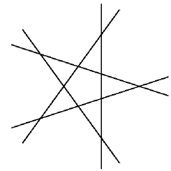
Figure 1: $R_{5}(x,y)=0$ in $\mathbb{P}^{2}$ and $z-R_{5}(x,y)=0$ in $\mathbb{P}^{3}$.

Then, Givental’s equations for cubics can be transferred word by word to obtain an affine equation for hyperquintics in $\mathbb{P}^{n}$ with many singular points (all are nodes):

$$\sum_{j=0}^{\lfloor\frac{n}{2}\rfloor-1}(-1)^{j\cdot(1+(n\bmod 2))}\widetilde{R}_{5}(x_{2j},x_{2j+1})=-(n\bmod 2)\frac{T_{5}(x_{n-1})-1}{2}\,,$$

where $T_{5}(z):=16z^{5}-20z^{3}+5z$ denotes the Tchebychev polynomial of degree $5$ with two critical values $\pm 1$ and $\widetilde{R}_{5}(x,y)$ is the normalized pentagon with critical value $+1$ over the origin. For a comparison of the resulting hyperquintics obtained by this method to our $\Sigma_{n+2}$-symmetric approach see table 3.

4.3 The $\Sigma_{n+2}$-symmetric Approach

We performed further experiments for some $n\not=4$, and it seems to us that the $\Sigma_{n+2}$-symmetric construction yields fewer nodes than the pentagon construction.

	number of ordinary nodes
$n$	$\Sigma_{n+2}$-symmetric approach	pentagon construction	$\operatorname{Ar}_{n}(5)$
3	20	31	31
4	130	126	135
5	210	420	456
6	1505	1620	1918
8	23436	23126	27876
10	296604	325580	411334

Table 3: Comparison of our $\Sigma_{n+2}$-symmetric approach and the pentagon construction in $\mathbb{P}^{n}$ for some $n$.

Indeed, the best hyperquintic $Q_{(7:-4)}$ in $\mathbb{P}^{5}$ contains only 210 ordinary nodes (cf. table 3); in $\mathbb{P}^{3}$, the best hyperquintic $Q_{(2:1)}$ has only 20 ordinary nodes. For $n=6$ and $n=10$ we obtained 1505 respectively 296604 ordinary nodes for the best examples. In $\mathbb{P}^{4}$ and $\mathbb{P}^{8}$, the $\Sigma_{n+2}$-symmetric approach yields hyperquintics with a higher number of ordinary nodes than the pentagon construction (cf. table 3).

We did not look at other $n$ in detail, we only verified that the number of generic nodes of the $\Sigma_{n+2}$-symmetric approach is less than the number of nodes obtained by using the pentagon construction. It is possible that for certain $n$ and $(\alpha:\beta)$ the $\Sigma_{n+2}$-symmetric construction is better.

Appendix

The Case Analysis

Here we list the remaining cases of the case analysis in section 2.

Case 3

Assume that $\eta=(1:1:1:1:1:1:1:1:-4:-4)$. Hence $C_{2}=40$, $C_{3}=-120$, $C_{4}=520$, and

$$P(X)=\textstyle X^{4}-40\lambda X^{2}+80\lambda X+160\lambda-52\,.$$

Via $P(1)=P(-4)=0$ we get $\lambda=\frac{51}{200}$, thus

$$(\alpha:\beta)=(100:-49)\,.$$

The length of the $\Sigma_{10}$-orbit of $\eta$ is $45={10\choose 2}$ .

Case 4

Consider $\eta=(a:a:a:a:a:a:a:a:b:-8a-b)$. For $a=0$ we get $\eta=(0:0:0:0:0:0:0:0:1:-1)$, hence $C_{2}=C_{4}=2$, $C_{3}=0$, and

$$\textstyle P(X)=X^{4}-2\lambda X^{2}+\frac{1}{5}(2\lambda-1)\,.$$

Requiring $P(0)=P(\pm 1)=0$ leads to $\lambda=\frac{1}{2}$, hence

$$(\alpha:\beta)=(1:0)\,.$$

The length of the $\Sigma_{10}$-orbit of $\eta$ is $45=\frac{1}{2}\cdot 10\cdot 9$.

For $a\not=0$ we have $\eta=(1:1:1:1:1:1:1:1:b:-8-b)$, hence $C_{2}=2b^{2}+16b+72$, $C_{3}=-24b^{2}-192b-504$, $C_{4}=2b^{4}+32b^{3}+384b^{2}+2048b+4104$, and $P$ appropriate. By requiring $P(1)=P(b)=P(-8-b)=0$, we obtain three equations for $\lambda$:

$$0= \lambda\cdot\big{(}\underbrace{2b^{4}+32b^{3}+342b^{2}+1712b+3912}_{=:a_{11}}\big{)}$$

$$\qquad+1\cdot\big{(}\underbrace{-b^{4}-16b^{3}-192b^{2}-1024b-2047}_{=:a_{12}}\big{)}$$

$$0= \lambda\cdot\big{(}\underbrace{-8b^{4}+32b^{3}+552b^{2}+2832b+2592}_{=:a_{21}}\big{)}$$

$$\qquad+1\cdot\big{(}\underbrace{4b^{4}-16b^{3}-192b^{2}-1024b-2052}_{=:a_{22}}\big{)}$$

$$0= \lambda\cdot\big{(}\underbrace{-8b^{4}-288b^{3}-3288b^{2}-16528b-33888}_{=:a_{31}}\big{)}$$

$$\qquad+1\cdot\big{(}\underbrace{4b^{4}+144b^{3}+1728b^{2}+9216b+18428}_{=:a_{32}}\big{)}$$

To have a unique solution for $\lambda$, the matrix

$$\left(\begin{array}[]{cc}a_{11}&a_{12}\\ a_{21}&a_{22}\\ a_{31}&a_{32}\end{array}\right)$$

must have rank 1. Thus, the three $2\times 2$ minors

$$\left|\begin{array}[]{cc}a_{11}&a_{12}\\ a_{21}&a_{22}\end{array}\right|\text{, }\left|\begin{array}[]{cc}a_{11}&a_{12}\\ a_{31}&a_{32}\end{array}\right|\text{, }\left|\begin{array}[]{cc}a_{21}&a_{22}\\ a_{31}&a_{32}\end{array}\right|$$

must vanish, which leads to

$$0=(b+9)(b-1)(b+4)(b^{2}+8b+27)\,.$$

The solutions 1 and $-9$ lead us back to case 2, $b=-4$ to case 3. If we take one of the two roots $b=-4\pm\sqrt{-11}$ of the remainig factor, $-8-b$ is the other one. Thus, the length of the $\Sigma_{10}$-orbit of $\eta$ is $90=10\cdot 9$.

Such an $\eta$ yields $C_{2}=18$, $C_{3}=144$, $C_{4}=-1350$, and

$$P(X)=X^{4}-18\lambda X^{2}-96\lambda X+\textstyle\frac{162}{5}\lambda+135\,.$$

Requiring $P(1)=P(-4\pm i\sqrt{11})=0$ leads to $3\lambda=5$ and

$$(\alpha:\beta)=(3:7)\,.$$

Case 5

Assume that $\eta=(3:3:3:3:3:3:3:-7:-7:-7)$. Hence $C_{2}=210$, $C_{3}=-840$, $C_{4}=7770$, and

$$P(X)=X^{4}-210\lambda X^{2}+560\lambda X+4410\lambda-777\,.$$

From $P(3)=P(-7)=0$ we get $\lambda=\frac{29}{175}$, hence

$$(\alpha:\beta)=(175:-117)\,.$$

The length of the $\Sigma_{10}$-orbit of $\eta$ is $120={10\choose 3}$ .

Case 6

Consider $\eta=(a:a:a:a:a:a:a:b:b:-7a-2b)$. For $a=0$ we put $b=1$, hence $C_{2}=6=-C_{3}$, $C_{4}=18$, and

$$\textstyle P(X)=X^{4}-6\lambda X^{2}+4\lambda X+\frac{18}{5}\lambda-\frac{9}{5}\,.$$

$P(0)=P(1)=P(-2)=0$ yields $\lambda=\frac{1}{2}$, hence

$$(\alpha:\beta)=(1:0)\,.$$

The length of the $\Sigma_{10}$-orbit of $\eta$ is $360=10\cdot{9\choose 2}$ .

For $a\not=0$, we have $\eta=(1:1:1:1:1:1:1:b:b:-7-2b)$. Thus,

$$C_{2} =6b^{2}+28b+56,$$

$$C_{3} =-6b^{3}-84b^{2}-294b-336,$$

$$C_{4} =18b^{4}+224b^{3}+1176b^{2}+2744b+2408,$$

and $P$ appropriate. By requiring $P(1)=P(b)=P(-2b-7)=0$, we again obtain three equations for $\lambda$ (cf. case 4), hence a $3\times 2$-matrix, which must have rank 1 to have a unique solution for $\lambda$. Thus, its three $2\times 2$-minors must vanish and we find

$$0=(b-1)(3b+7)(b+4)(3b^{4}+39b^{3}+189b^{2}+413b+364)\,.$$

The solutions $b\in\{\,1,-4,-\frac{7}{3}\,\}$ lead us back into cases 2, 3, and 5, respectively. For $b$ a root of the remaining factor and by $P(1)=P(b)=P(-2b-7)=0$, we obtain $\lambda=\frac{-1}{168}(3b^{3}+15b^{2}-39b-259)$, hence

$$(\alpha:\beta)=(84:-3b^{3}-15b^{2}+39b+175)\,.$$

The length of the $\Sigma_{10}$-orbit of $\eta$ is $360=10\cdot{9\choose 2}$.

Case 8

We consider $\eta=(2:2:2:2:2:2:-3:-3:-3:-3)$ and obtain $C_{2}=-C_{3}=60$, $C_{4}=420$, and, thus,

$$P(X)=X^{4}-60\lambda X^{2}+40\lambda X+360\lambda-42\,.$$

$P(2)=P(-3)=0$ leads to $\lambda=\frac{13}{100}$, hence

$$(\alpha:\beta)=(50:-37)\,.$$

The length of the $\Sigma_{10}$-orbit of $\eta$ is $210={10\choose 4}$.

Case 9

Assume that $\eta=(a:a:a:a:a:a:b:b:b:-6a-3b)$. For $a=0$, $b=1$ we find $C_{2}=12$, $C_{3}=-24$, $C_{4}=84$, and

$$P(X)=X^{4}-12\lambda X^{2}+16\lambda X+\textstyle\frac{72}{5}\lambda-\frac{42}{5}\,,$$

but for no $\lambda$ does $P(0)=P(1)=P(-3)=0$ hold simultaneously.

For $\eta=(1:1:1:1:1:1:b:b:b:-3b-6)$ we obtain

$$C_{2} =12b^{2}+36b+42,$$

$$C_{3} =-24b^{3}-162b^{2}-324b-210,$$

$$C_{4} =84b^{4}+648b^{3}+1944b^{2}+2592b+1302$$

and $P$ appropriate. Equating $P(X)$ to zero for $X=1,b,-3b-6$ leads to an equation system for $\lambda$ again (cf. cases 4 and 6), hence a $3\times 2$-matrix, whose three $2\times 2$-minors must vanish to have a unique solution for $\lambda$. Thus,

$$0=(3b+7)(b-1)(2b+3)(b+2)(2b^{4}+25b^{3}+93b^{2}+139b+77)\,.$$

The first three factors take us back into cases 5, 2, and 8, respectively, for $b=-2$ we find $C_{2}=-C_{3}=18$, $C_{4}=54$, and

$$\textstyle P(X)=X^{4}-18\lambda X^{2}+12\lambda X+\frac{162}{5}\lambda-\frac{27}{5}\,.$$

Requiring $P(1)=P(-2)=P(0)=0$ yields $\lambda=\frac{1}{6}$, hence

$$(\alpha:\beta)=(3:-2)\,.$$

The length of the $\Sigma_{10}$-orbit of $\eta$ is $840=10\cdot{9\choose 3}$.

For $b$ a root of the remaining factor, we find $\lambda=\frac{1}{42}(2b^{3}+25b^{2}+86b+97)$ by requiring $P(1)=P(b)=P(-3b-6)=0$. Thus,

$$(\alpha:\beta)=(21:2b^{3}+25b^{2}+86b+76)\,.$$

The length of the $\Sigma_{10}$-orbit of $\eta$ also is $840=10\cdot{9\choose 3}$ here.

Case 10

Assume that $\eta=(a:a:a:a:a:a:b:b:c:c)$ with $3a+b+c=0$ . For $a=0$, $b=-c=1$ we find $C_{2}=C_{4}=4$, $C_{3}=0$, and

$$P(X)=X^{4}-4\lambda X^{2}+\textstyle\frac{8}{5}\lambda-\frac{2}{5}\,.$$

Via $P(0)=P(\pm 1)=0$ we find $\lambda=\frac{1}{4}$, hence

$$(\alpha:\beta)=(2:-1)\,.$$

The length of the $\Sigma_{10}$-orbit of $\eta$ is $630=\frac{1}{2}\cdot{10\choose 2}{8\choose 2}$ .

For $a=1$, $c=-3-b$ we find $C_{2}=4(b^{2}+3b+6)$, $C_{3}=-6(3b^{2}+9b+8)$, $C_{4}=4(b^{4}+6b^{3}+27b^{2}+54b+42)$, and $P$ appropriate. The conditions on the coordinates of $\eta$ produce three equations for $\lambda$. By the same method as in cases 4, 6, and 9, we obtain

$$0=(b+4)(b-1)(2b+3)(b^{2}+3b+4)\,.$$

The linear factors lead us back to cases 3 and 8. For a root $b=\frac{-3\pm\sqrt{-7}}{2}$ of the last factor, $-b-3$ is the other one. Hence, the length of the $\Sigma_{10}$-orbit of $\eta$ is $1260={10\choose 2}{8\choose 2}$.

Such an $\eta=(2:2:2:2:2:2:2b:2b:-6-2b:-6-2b)$ implies $C_{2}=32$, $C_{3}=192$, $C_{4}=-896$, and

$$P(X)=X^{4}-32\lambda X^{2}-128\lambda X+\textstyle\frac{512}{5}\lambda+\frac{448}{5}\,.$$

By $P(2)=P(2b)=P(-6-2b)=0$ we find $\lambda=\frac{3}{8}$, hence

$$(\alpha:\beta)=(4:-1)\,.$$

Case 11

Assume that $\eta=(a:a:a:a:a:a:b:b:c:d)$. Due to $6a+2b+c+d=a+b+c+d=0$, we obtain $b=-5a$ and $d=4a-c$ .

$a=0$ takes us back to case 4, so we put $a=1$. This leads to

$$C_{2} =2c^{2}-8c+72,$$

$$C_{3} =12c^{2}-48c-180,$$

$$C_{4} =2c^{4}-16c^{3}+96c^{2}-256c+1512,$$

and $P$ appropriate. By the conditions on $P$ we find

$5c^{2}-20c+27=0$  and  $51\lambda=13$ .

For a root $c=2\pm\sqrt{-\frac{7}{5}}$ , the other one is $4-c$. Hence, we obtain

$$(\alpha:\beta)=(51:-25)$$

and an orbit length of $\eta$ of $2520=10\cdot 9\cdot{8\choose 2}$.

Case 13

Consider $\eta=(a:a:a:a:a:b:b:b:b:-5a-4b)$. For $a=0$ and $b=1$ we find $C_{2}=20$, $C_{3}=-60$, $C_{4}=260$, and

$$P(X)=X^{4}-20\lambda X^{2}+40\lambda X+40\lambda-26\,.$$

Requiring $P(0)=P(1)=P(-4)=0$ leads to a contradiction.

For $a=1$ we have $C_{2}=20b^{2}+40b+30$, $C_{3}=-60b^{3}-240b^{2}-300b-120$, $C_{4}=260b^{4}+1280b^{3}+2400b^{2}+2000b+630$, and $P$ appropriate. If we require $P(1)=P(b)=P(-4b-5)=0$, we obtain the following equations:

$$0= (b-1)(b+1)^{3}(2b+3)(7b^{2}+29b+27)\,,$$

$$0= (b+1)(450\lambda+182b^{5}+1055b^{4}+1795b^{3}+145b^{2}-2055b-1368)\,.$$

The solutions $b\in\{1,-1,-\frac{3}{2}\}$ of the first equation lead us back to cases 2, 12, and 8, respectively, the roots $b=\frac{-29\pm\sqrt{85}}{14}$ of the remaining factor together with the second equation imply $\lambda=-\frac{7}{30}b-\frac{1}{5}=\frac{17\mp\sqrt{85}}{60}$, hence

$$(\alpha:\beta)=(30:-13\mp\sqrt{85})\,.$$

Here, the length of the $\Sigma_{10}$-orbit of $\eta$ is $1260=10\cdot{9\choose 4}$ .

Case 14

Assume that $\eta=(a:a:a:a:a:b:b:b:c:c)$. For $a=0$, $b=2$ we obtain $C_{2}=-C_{3}=30$, $C_{4}=210$, and

$$P(X)=X^{4}-30\lambda X^{2}+20\lambda X+90\lambda-21\,.$$

Requiring $P(0)=P(2)=P(-3)=0$, however, leads to a contradiction.

For $\eta=(2:2:2:2:2:2b:2b:2b:-5-3b:-5-3b)$ we find $C_{2}=10(3b^{2}+6b+7)$, $C_{3}=-30(b+7)(b+1)^{2}$, $C_{4}=10(21b^{4}+108b^{3}+270b^{2}+300b+133)$, and $P$ appropriate. Requiring $P(2)=P(2b)=P(-5-3b)=0$ implies

$$0=(b+1)(78400\lambda-186b^{5}+85b^{4}+4265b^{3}+6565b^{2}-6235b-24486)\,,$$

$$0=(b-1)(b+1)^{3}(3b+7)(b^{2}-3b-14)\,.$$

The roots $b\in\{\,1,-1,-\frac{7}{3}\,\}$ of the second equation take us back to cases 3, 12, and 5, respectively. The roots $b=\frac{3\pm\sqrt{65}}{2}$ of the remaining factor of the second equation, however, imply $\lambda=\frac{117\pm 3\sqrt{65}}{560}$ via the first equation, hence

$$(\alpha:\beta)=(280:-163\pm 3\sqrt{65})\,.$$

The length of the $\Sigma_{10}$-orbit of $\eta$ is $2520={10\choose 2}{8\choose 3}$ .

Case 15

Due to $5a+3b+c+d=a+b+c+d=0$ we may assume $\eta=(a:a:a:a:a:-2a:-2a:-2a:c:a-c)$. For $a=0$ we are taken to case 4.

For $a=1$ we find $C_{2}=2(c^{2}-c+9)$, $C_{3}=3(c^{2}-c-6)$, $C_{4}=2(c^{4}-2c^{3}+3c^{2}-2c+27)$, and $P$ appropriate. But $P(1)=P(-2)=P(c)=P(1-c)=0$ imply $0=c(c-1)$ and $6\lambda=1$ , and both $c=0$ and $c=1$ lead to case 9.

Case 16

Due to $5a+2b+2c+d=a+b+c+d=0$ we may assume $\eta=(a:a:a:a:a:b:b:-4a-b:-4a-b:3a)$. Since $a=0$ leads to case 10, we put $a=1$ and obtain $C_{2}=2(b^{2}+8b+23)$, $C_{3}=-24(b+2)^{2}$, $C_{4}=4b^{4}+32b^{3}+192b^{2}+512b+598$, and $P$ appropriate. Requiring $P(1)=P(b)=P(3)=P(-4-b)=0$, we find $b^{2}+4b+7=0$ and $\lambda=\frac{1}{3}$, hence

$$(\alpha:\beta)=(3:-1)\,.$$

For $b=-2\pm\sqrt{-3}$ one of the two solutions, $-4-b$ is the other one, so we find $7560=10\cdot{9\choose 2}{7\choose 2}$ elements in the $\Sigma_{10}$-orbit of $\eta$.

Case 17

Assume that $\eta=(a:a:a:a:b:b:b:b:-2a-2b:-2a-2b)$. For $a=0$, $b=1$ we find $C_{2}=-C_{3}=12$, $C_{4}=36$, and

$$P(X)=X^{4}-12\lambda X^{2}+8\lambda X+\textstyle\frac{72}{5}\lambda-\frac{18}{5}\,.$$

Via $P(0)=P(1)=P(-2)=0$ we immediately obtain $\lambda=\frac{1}{4}$, hence

$$(\alpha:\beta)=(2:-1)\,.$$

The length of the $\Sigma_{10}$-orbit of $\eta$ is $3150={10\choose 2}{8\choose 4}$ .

For $a=1$ we find $C_{2}=4(3b^{2}+4b+3)$, $C_{3}=-12(b^{3}+4b^{2}+4b+1)$, $C_{4}=4(9b^{4}+32b^{3}+48b^{2}+32b+9)$, and $P$ appropriate. Requiring $P(1)=P(b)=P(-2b-2)=0$, we obtain

$$0=b(b-1)(b+1)^{3}(3b+2)(2b+3)\,,$$

$$0=400\lambda+210b^{6}+695b^{5}+556b^{4}-377b^{3}-742b^{2}-344b-100\,. (*)$$

The case $b=0$ is checked above, whereas $b=1$ and $b\in\{-\frac{2}{3},-\frac{3}{2}\}$ take us back to cases 3 and 8, respectively. For $b=-1$ we obtain $\lambda=\frac{1}{8}$ via $(*)$, hence

$$(\alpha:\beta)=(4:-3)\,.$$

The length of the $\Sigma_{10}$-orbit of $\eta$ is $1575=\frac{1}{2}\cdot{10\choose 4}{6\choose 4}$ .

Case 19

We may assume $\eta=(3a:3a:3a:3a:b:b:b:-4a-b:-4a-b:-4a-b)$. For $a=0$, $b=1$ we find $C_{2}=C_{4}=6$, $C_{3}=0$, and

$$P(X)=\textstyle X^{4}-6\lambda X^{2}+\frac{18}{5}\lambda-\frac{3}{5}\,.$$

$P(0)=P(\pm 1)=0$ leads to $\lambda=\frac{1}{6}$, hence

$$(\alpha:\beta)=(3:-2)\,.$$

The length of the $\Sigma_{10}$-orbit of $\eta$ is $2100=\frac{1}{2}\cdot{10\choose 3}{7\choose 3}$.

For $a=1$ we find $C_{2}=6(b^{2}+4b+14)$, $C_{3}=-12(3b^{2}+12b+7)$, $C_{4}=6(b^{4}+8b^{3}+48b^{2}+128b+182)$, and $P$ appropriate. Requiring $P(3)=P(b)=P(-4-b)=0$ leads to

$$0 =(b-3)(b+2)(b+7)(b^{2}+4b+7)\,,$$

$$0 =4900\lambda-b^{4}-8b^{3}-6b^{2}+40b-581\,.$$

The solutions $b\in\{\,-7,-2,3\,\}$ of the first equation take us back to cases 5 and 8, respectively. If $b$ is one of the two remaining roots $-2\pm\sqrt{-3}$ of the first equation, $-4-b$ is the other one. Hence, the length of the $\Sigma_{10}$-orbit of $\eta$ is $4200={10\choose 3}{7\choose 3}$ . Furthermore, by the second equation we obtain $\lambda=\frac{1}{7}$, hence

$$(\alpha:\beta)=(7:-5)\,.$$

Case 20

Due to $4a+3b+2c+d=a+b+c+d=0$ we have $c=-3a-2b$, $d=2a+b$, and $\eta=(a:a:a:a:b:b:b:-3a-2b:-3a-2b:2a+b)$. Since $a=0$ takes us to case 17, we put $a=1$ and obtain

$$C_{2} =12b^{2}+28b+26,$$

$$C_{3} =-12b^{3}-66b^{2}-96b-42,$$

$$C_{4} =36b^{4}+200b^{3}+456b^{2}+464b+182,$$

and $P$ appropriate. Equating $P(X)$ to zero for $X=1,b,-3-2b,2+b$, we find

$$0 =(b+1)^{3}(b+2)\,,$$

$$0 =(b+1)(300\lambda+11b^{3}+18b^{2}-33b-100)\,.$$

The two solutions $b\in\{-2,-1\}$ of the first equation lead us back to cases 9 and 12, respectively.

Case 21

Since we have $2a+b+c+d=a+b+c+d=0$, we immediately may assume $\eta=(0:0:0:0:b:b:c:c:-b-c:-b-c)$. As $b$ and $c$ cannot vanish simultaneously, w.l.o.g. we put $b=1$ and find $C_{2}=4(c^{2}+c+1)$, $C_{3}=-6c(c+1)$, $C_{4}=4(c^{2}+c+1)^{2}$, and $P$ appropriate. $P(0)=P(1)=P(c)=P(-1-c)=0$ imply $\lambda=\frac{1}{4}$, so

$$(\alpha:\beta)=(2:-1)\,.$$

We thus have found $3150=\frac{1}{3!}{10\choose 2}{8\choose 2}{6\choose 2}$ singular lines, since there are no further conditions on $c\in\mathbb{C}$ .

Case 22

Due to $3a+3b+3c+d=a+b+c+d=0$ we have $a+b+c=0=d$ and, hence, $\eta=(a:a:a:b:b:b:-a-b:-a-b:-a-b:0)$. Since $a=0$ leads us back to case 19, we put $a=1$ and find $C_{2}=6(b^{2}+b+1)$, $C_{3}=-9b(b+1)$, $C_{4}=6(b^{2}+b+1)^{2}$, and $P$ appropriate. Requiring $P(0)=P(1)=P(b)=P(-1-b)=0$, we obtain $\lambda=\frac{1}{6}$, hence

$$(\alpha:\beta)=(3:-2)\,.$$

Since there are no further conditions on $b\in\mathbb{C}$ , we again have found $2800=\frac{1}{3!}{10\choose 3}{7\choose 3}{4\choose 3}$ singular lines.

Case 23

Due to $3a+3b+2c+2d=a+b+c+d=0$ we have $b=-a$, $d=-c$ and, hence, may assume $\eta=(a:a:a:-a:-a:-a:c:c:-c:-c)$. For $a=0$ we are back in case 10, so we put $a=1$. Thus, we find $C_{2}=4c^{2}+6$, $C_{3}=0$, $C_{4}=4c^{4}+6$, and $P$ appropriate. Via $P(\pm c)=P(\pm 1)=0$ we obtain

$$0=\big{(}2\lambda(2c^{2}+3)-(c^{2}+1)\big{)}(c+1)(c-1)\,.$$

With $c=\pm 1$ we are back in case 12, so we assume $c\not=\pm 1$. Thus,

$$0=(4\lambda-1)c^{2}+(6\lambda-1)\,.$$

This equation has no solution for $\lambda=\frac{1}{4}$, but for $\lambda\not=\frac{1}{4}$ we have

$$0=(\alpha+2\beta)c^{2}+(2\alpha+3\beta)\,. \hskip 71.13188pt(*)$$

So $\eta$ is a singular point of $Q_{(\alpha:\beta)}$, $(\alpha:\beta)\not=(2:-1)$, for all $c\in\mathbb{C}$ that satisfy $(*)$ and we have found $12600=\frac{1}{2}\cdot{10\choose 3}{7\choose 3}{4\choose 2}$ more generic singularities of $Q_{(\alpha:\beta)}$ in $\mathbb{P}^{8}$ (cf. [Schm] and the cases 12 and 18).

If $(\alpha:\beta)\in\{\,(5:-3),(3:-2)\,\}$ , which means $\lambda\in\{\,\frac{1}{5},\frac{1}{6}\,\}$, the solutions of $(*)$ are $c=\pm 1$ and $c=0$, respectively, so two respective orbit elements of $\eta$ merge or they coincide with the singular points from case 12. Hence, we have singularities that are worse than ordinary nodes. A proof of this is given in section 3.
For this reason, we add $(\alpha:\beta)\in\{\,(2:-1),(5:-3),(3:-2)\,\}$  and $\lambda\in\{\,\frac{1}{4},\frac{1}{5},\frac{1}{6}\,\}$ to the exceptional values introduced in case 18. The cases 21 and 22, however, already showed that we have singular lines contained in $Q_{(2:-1)}$ and $Q_{(3:-2)}$.

References

- [AGZV] V.I. Arnold, S.M. Gusein-Zade, A.N. Varchenko, Singularities of differential maps, Birkhäuser, 1985
- [Bar] W. Barth, Two Projective Surfaces with Many Nodes, Admitting the Symmetry of the Icosahedron, J. Algebraic Geom. 5 (1996), no. 1, 173–186
- [Gor] V.V. Goryunov, Symmetric Quartics with many Nodes, Advances in Soviet Mathematics, Volume 21, 1994, 147–161
- [Hir] F. Hirzebruch, Some Examples of Threefolds with trivial canonical bundle, in Collected Works Vol. II (1995), Springer Verlag, 757–770
- [JR] D.B. Jaffe, D. Ruberman, A Sextic Surface cannot have 66 Nodes, J. Algebraic Geom. 6 (1997), no. 1, 151–168
- [Kal] T. Kalker, Cubic Fourfolds with 15 Ordinary Double Points, Ph. D. thesis, Leiden, 1986
- [Lab] O. Labs, Hypersurfaces with many Singularities, Ph. D. thesis, Mainz, available from www.OliverLabs.net, 2005
- [Schm] O. Schmidt, Symmetrische Quintiken mit vielen Doppelpunkten, Diploma thesis, Mainz, 2006
- [vStr] D. van Straten, A Quintic Hypersurface in with 130 Nodes, Topology 32 (1993), No. 4, 857–864
- [Var] A.N. Varchenko, On the Semicontinuity of the Spectrum and an Upper Bound for the Number of Singular Points of a Projective Hypersurface, J. Soviet Math. 270 (1983), 735–739