Quantum state tomography via compressed sensing

Abstract

We establish methods for quantum state tomography based on compressed sensing. These methods are specialized for quantum states that are fairly pure, and they offer a significant performance improvement on large quantum systems. In particular, they are able to reconstruct an unknown density matrix of dimension $d$ and rank $r$ using $O(rd\log^{2}d)$ measurement settings, compared to standard methods that require $d^{2}$ settings. Our methods have several features that make them amenable to experimental implementation: they require only simple Pauli measurements, use fast convex optimization, are stable against noise, and can be applied to states that are only approximately low-rank. The acquired data can be used to certify that the state is indeed close to pure, so no a priori assumptions are needed. We present both theoretical bounds and numerical simulations.

The tasks of reconstructing the quantum states and processes produced by physical systems — known respectively as quantum state and process tomography Paris2004 — are of increasing importance in physics and especially in quantum information science. Tomography has been used to characterize the quantum state of trapped ions Haffner2005 and an optical entangling gate OBrien2003 among many other implementations. But a fundamental difficulty in performing tomography on many-body systems is the exponential growth in the state space dimension. For example, to get a maximum-likelihood estimate of a quantum state of $8$ ions, Ref. Haffner2005 required hundreds of thousands of measurements and weeks of post-processing.

Still, one might hope to overcome this obstacle, because the vast majority of quantum states are not of physical interest. Rather, one is often interested in states with special properties: pure states, states with particular symmetries, ground states of local Hamiltonians, etc., and tomography might be more efficient in such special cases Kaznady2009 .

In particular, consider pure or nearly pure quantum states, i.e., states with low entropy. More precisely, consider a quantum state that is essentially supported on an $r$-dimensional space, meaning the density matrix is close (in a given norm) to a matrix of rank $r$, where $r$ is small. Such states arise in very common physical settings, e.g. a pure state subject to a local noise process localnoise .

A standard implementation of tomography S1 ; S2 would use $d^{2}$ or more measurement settings, where $d=2^{n}$ for an $n$-qubit system. But a simple parameter counting argument suggests that $O(rd)$ settings could possibly suffice — a significant improvement. However, it is not clear how to achieve this performance in practice, i.e., how to choose these measurements, or how to efficiently reconstruct the density matrix. For instance, the problem of finding a minimum-rank matrix subject to linear constraints is NP-hard in general natarajan95 .

In addition to a reduction in experimental complexity, one might hope that a post-processing algorithm which takes as input only $O(rd)\ll d^{2}$ numbers could be tuned to run considerably faster than standard methods. Since the output of the procedure is a low-rank approximation to the density operator and only requires $O(rd)$ numbers be specified, it becomes conceivable that the run time scales better than $O(d^{2})$, clearly impossible for naive approaches using dense matrices.

In this Letter, we introduce a method to achieve such drastic reductions in measurement complexity, together with efficient algorithms for post-processing. The approach further develops ideas that have recently been studied under the label of “compressed sensing”. Compressed sensing compressedsensing provides techniques for recovering a sparse vector from a small number of measurements Kosut2008 . Here, sparsity means that this vector contains only a few non-zero entries in a specified basis, and the measurements are linear functions of its entries. When the measurements are chosen at random (in a certain precise sense), then with high probability two surprising things happen: the vector is uniquely determined by a small number of measurements, and it can be recovered by an efficient convex optimization algorithm compressedsensing .

Matrix completion Candes2008 ; Candes2009a ; Candes2009 is a generalization of compressed sensing from vectors to matrices. Here, one recovers certain “incoherent” low-rank matrices $X$ from a small number of matrix elements $X_{i,j}$. The problem of low-rank quantum state tomography bears a strong resemblance to matrix completion. However, there are important differences. We wish to use measurements that can be more easily implemented in an experiment than obtaining elements $\rho_{i,j}$ of density matrices. Previous results Candes2008 ; Candes2009a ; Candes2009 cannot be applied to this more general situation. We would also like to avoid any unnatural incoherence assumptions crucial in prior work Candes2008 .

Our first result is a protocol for tomography that overcomes both of these difficulties: it uses Pauli measurements only, and it works for arbitrary density matrices. We prove that only $O(rd\,\log^{2}d)$ measurement settings suffice. What is more, our proof introduces some new techniques, which both generalize and vastly simplify the previous work on matrix completion. We sketch the proof here; a more complete version appears in prep2 . This provides the basic theoretical justification for our method of doing tomography.

We then consider a number of practical issues. In a real experiment, the measurements are noisy, and the true state is only approximately low-rank. We show that our method is robust to these sources of error. We also describe ways to certify that a state is nearly pure without any a priori assumptions.

Finally, we present fast algorithms for reconstructing the density matrix from the measurement statistics based on semidefinite programming – a feature not present in earlier methods for pure-state tomography Kaznady2009 ; S1 ; S2 . These are adapted from algorithms for matrix completion Cai2008 , and they are much faster than standard interior-point solvers. Reconstructing a low-rank density matrix for $8$ qubits takes about one minute on an ordinary laptop computer.

While our methods do not overcome the exponential growth in measurement complexity (which is provably impossible for any protocol capable of handling generic pure states), they do significantly push the boundary of what can be done in a realistic setting.

Our techniques also apply to process tomography: to characterize an unknown quantum process $\mathcal{E}$, prepare the Jamiołkowski state $\rho_{\mathcal{E}}$, and perform state tomography on $\rho_{\mathcal{E}}$. Our methods work when $\mathcal{E}$ can approximately be written as a sum of only a few Kraus operators, because this implies that $\rho_{\mathcal{E}}$ has small rank.

Matrix recovery using Pauli measurements.

We consider the case of $n$ spin-$1/2$ systems in an unknown state $\rho$ note1 . An $n$-qubit Pauli matrix is of the form $w=\bigotimes_{i=1}^{n}w_{i}$, where $w_{i}\in\{\mathbbm{1},\sigma^{x},\sigma^{y},\sigma^{z}\}$. There are $d^{2}$ such matrices, labeled $w(a),a\in[1,d^{2}]$. The protocol proceeds as follows: choose $m$ integers $A_{1},\dots,A_{m}\in[1,d^{2}]$ at random and measure the expectation values $\operatorname{tr}\rho w(A_{i})$. One then solves a convex optimization problem: minimize $\|\sigma\|_{\operatorname{tr}}$ note2 subject to

$$\operatorname{tr}\sigma=1,\qquad\operatorname{tr}w(A_{i})\sigma=\operatorname{tr}w(A_{i})\rho.$$ (1)

Theorem 1 (Low-rank tomography)

Let $\rho$ be an arbitrary state of rank $r$. If $m=cdr\log^{2}d$ randomly chosen Pauli expectations are known, then $\rho$ can be uniquely reconstructed by solving the convex optimization problem (1) with probability of failure exponentially small in $c$.

The proof is inspired by, but technically very different from, earlier work on matrix completion Candes2008 . Our methods are more general, can be tuned to give tighter bounds, and are much more compact, allowing us to present a fairly complete argument in this Letter. A more detailed presentation of this technique – covering the reconstruction of low-rank matrices from few expansion coefficients w.r.t. general operator bases (not just Pauli matrices or matrix elements) – will be published elsewhere prep2 .

Proof: Here we sketch the argument and explain the main ideas; detailed calculations are in the EPAPS supplement.

Note that the linear constraints (1) depend only on the projection of $\rho$ onto the span of the measured observables $w(A_{1}),\dots,w(A_{m})$. This is precisely the range of the “sampling operator” $\mathcal{R}:\rho\mapsto\frac{d}{m}\sum_{i=1}^{m}w(A_{i})\operatorname{tr}\rho w(A_{i})$. (Note that $\mathbbm{E}[\mathcal{R}(\rho)]=\rho$.) Indeed, the convex program can be written as $\min_{\sigma}\|\sigma\|_{\operatorname{tr}}$ s.t. $\mathcal{R}\sigma=\mathcal{R}\rho$. Evidently, the solution is unique if for all deviations $\Delta:=\sigma-\rho$ away from $\rho$ either $\mathcal{R}\Delta\neq 0$ or $\|\rho+\Delta\|_{\operatorname{tr}}>\|\rho\|_{\operatorname{tr}}$.

We will ascertain this by using a basic idea from convex optimization: constructing a strict subgradient $Y$ for the norm. A matrix $Y$ is a strict subgradient if $\|\rho+\Delta\|_{\operatorname{tr}}>\|\rho\|_{\operatorname{tr}}+\operatorname{tr}Y\Delta$ for all $\Delta\neq 0$. The main contribution below is a method for constructing such a $Y$ which is also in the range of $\mathcal{R}$. For then $\mathcal{R}\Delta=0$ implies that $\Delta$ is orthogonal to the range of $\mathcal{R}$, thus $\operatorname{tr}Y\Delta=0$ and the subgradient condition reads $\|\rho+\Delta\|_{\operatorname{tr}}>\|\rho\|_{\operatorname{tr}}$. This implies uniqueness. (In fact, it is sufficient to approximate the subgradient condition in a certain sense).

Let $E$ be the projection onto the range of $\rho$, let $T$ be the space spanned by those operators whose row or column space is contained in $\operatorname{range}\rho$. Let $\mathcal{P}_{T}$ be the projection onto $T$, $\mathcal{P}_{T}^{\bot}$ onto the orthogonal complement. Decompose $\Delta=\Delta_{T}+\Delta_{T}^{\bot}$, the parts of $\Delta$ that lie in the subspaces $T$ and $T^{\bot}$. We distinguish two cases: (i) $\|\Delta_{T}\|_{2}>d^{2}\|\Delta_{T}^{\bot}\|_{2}$, and (ii) $\|\Delta_{T}\|_{2}\leq d^{2}\|\Delta_{T}^{\bot}\|_{2}$ note2 .

Case (i) is easier. In this case, $\Delta$ is well-approximated by $\Delta_{T}$ and essentially we only have to show that the restriction $\mathcal{A}:=\mathcal{P}_{T}\mathcal{R}\mathcal{P}_{T}$ of $\mathcal{R}$ to $T$ is invertible. Using a non-commutative large deviation bound (see EPAPS supplement),

$$\Pr[\|\mathcal{A}-\mathbbm{1}_{T}\|>t]<4dre^{-t^{2}\kappa/8}$$ (2)

where $\kappa=m/(dr)$ note2 . Hence the probability that $\|\mathcal{A}-\mathbbm{1}_{T}\|>\frac{1}{2}$ is smaller than $4dre^{-\kappa/32}=:p_{1}$. If that is not the case, one easily sees that $\|\mathcal{R}\Delta\|_{2}>0$, concluding the proof for this case.

Case (ii) is more involved. A matrix $Y\in\operatorname{span}(w(A_{1}),\ldots,w(A_{m}))$ is an almost subgradient note3 if

$$\|\mathcal{P}_{T}Y-E\|_{2}\leq 1/(2d^{2}),\qquad\|\mathcal{P}_{T}^{\bot}Y\|<1/2.$$ (3)

First, suppose such a $Y$ exists. Then a simple calculation (see EPAPS) using the condition (ii) shows that $\mathcal{R}\Delta=0$ indeed implies $\|\rho+\Delta\|_{\operatorname{tr}}>\|\rho\|_{\operatorname{tr}}$ as hinted at above. This proves uniqueness in case (ii). The difficult part consists in showing that an almost-subgradient exists.

To this end, we design a recursive process (the “golfing scheme” prep2 ) which converges to a subgradient exponentially fast. Assume we draw $l$ batches of $\kappa_{0}rd$ Pauli observables independently at random ($\kappa_{0}$ will be chosen later). Define recursively $X_{0}=E$,

$$Y_{i}=\sum_{j=1}^{i}\mathcal{R}_{j}X_{j-1},\quad X_{i}=E-\mathcal{P}_{T}Y_{i},$$ (4)

$Y=Y_{l}$. Let $\mathcal{R}_{i}$ be the sampling operator associated with the $i$th batch, and $\mathcal{A}_{i}$ its restriction to $T$. Assume that in each run $\|\mathcal{A}_{i}-\mathbbm{1}_{T}\|_{2}<1/2$. Denote the probability of this event not occurring by $p_{2}$. Then

$$\|X_{i}\|_{2} = \|X_{i-1}-\mathcal{P}_{T}\mathcal{R}_{i}X_{i-1}\|_{2}$$

$$= \|(\mathbbm{1}_{T}-\mathcal{A}_{i})X_{i-1}\|_{2}\leq 1/2\|X_{i-1}\|_{2},$$

so that $\|X_{i}\|_{2}\leq 2^{-i}\|X_{0}\|=2^{-i}\sqrt{r}$. Hence, $Y=Y_{l}$ fulfills the first part of (3), as soon as $l\geq\log_{2}(2d^{2}\sqrt{r})$. We turn to the second part. Again using large-deviation techniques (EPAPS) we find $\|\mathcal{P}_{T}^{\bot}\mathcal{R}_{i}X_{i-1}\|\leq 1/(4\sqrt{r})\|X_{i-1}\|_{2}$ with some (high) probability $(1-p_{3})$. Therefore:

$$\|\mathcal{P}_{T}^{\bot}Y_{l}\|\leq\sum_{j=1}^{l}\|\mathcal{P}_{T}^{\bot}\mathcal{R}_{j}X_{j-1}\|\leq\frac{1}{4}\sum_{j=0}^{\infty}2^{-l}<\frac{1}{2},$$ (5)

which is the second part of (3).

Lastly, we have to bound the total probability of failure $p_{f}\leq p_{1}+p_{2}+p_{3}$. Set $\kappa_{0}=64\mu(1+\ln(8dl))$, which means that $m=dr(\ln d)^{2}\,O(1)$ coefficients will be sampled in total. A simple calculation gives $p_{f}\leq e^{-\mu}$. This completes the proof of our main result. $\Box$

In the remaining space, we address the important aspects of resilience against noise, certified tomography, and numerical performance. Owing to space limitations, the presentation will focus on conceptual issues, with the details in prep1 .

Robustness to noise.

Realistic situations will differ from the previous case in two regards. First, the true state $\rho_{t}$ may not be low-rank, but only well approximated by a state $\rho$ of rank $r$: $\|\rho_{t}-\rho\|_{2}\leq\varepsilon_{1}$. Second, due to systematic and statistical noise, the available estimates for the Pauli expectations are not exactly $\operatorname{tr}\rho_{t}w(a)$, but of the form $\operatorname{tr}\omega w(a)$ for some matrix $\omega$. Assume $\|\mathcal{R}\omega-\mathcal{R}\rho_{t}\|_{2}\leq\varepsilon_{2}$ (in practical situations, $\varepsilon_{2}$ may be estimated from the error bars associated with the individual Pauli expectation values errormodel ). In order to get an estimate for $\rho_{t}$, choose some $\lambda\geq 1$ and $\varepsilon\geq\lambda(\sqrt{d^{2}/m})\varepsilon_{1}+\varepsilon_{2}$, and solve the convex program

$$\min\|\sigma\|_{\operatorname{tr}}\ ,\ \text{subject to}\,\|\mathcal{R}\sigma-\mathcal{R}\omega\|_{2}\leq\varepsilon.$$ (6)

Observation 1 (Robustness to noise)

Let $\rho_{t}$ be an approximately low-rank state as described above. Suppose $m=cdr\log^{2}d$ randomly chosen Pauli expectations are known up to an error of $\varepsilon$ as in (6), and let $\sigma^{\star}$ be the solution of (6). Then the difference $\|\sigma^{\star}-\rho_{t}\|_{\operatorname{tr}}$ is smaller than $O(\varepsilon\sqrt{rd})$. This holds with probability of failure at most $1/\lambda^{2}$ plus the probability of failure in Theorem 1.

The proof combines ideas from Ref. Candes2009 with our argument above note4 . The main difference from the noise-free case is that, instead of using $\operatorname{tr}Y\Delta=0$, we must now work with $|\operatorname{tr}Y\Delta|\leq 2\|Y\|_{2}\,\delta$. With this estimate, Observation 1 follows from the noise-free proof, together with some elementary calculations (see EPAPS). We remark that the above bound is likely to be quite loose; based on related work involving the “restricted isometry property,” we conjecture that the robustness to noise is actually substantially stronger than what is shown here FCRP08 .

Certified tomography of almost pure states.

The preceding results require an a priori promise: that the true state $\rho_{t}$ is $\delta_{1}$-close to a rank-$r$ state. However, when performing tomography of an unknown state, neither $r$ nor $\delta_{1}$ are known beforehand. There are a few solutions to this quandary. First, $r$ and $\delta_{1}$ may be estimated from other physical parameters of the system, such as the strength of the local noise localnoise .

Another approach is to estimate $r$ and $\delta_{1}$ from the same data that is used to reconstruct the state. When $r=1$, this approach is particularly effective, in entirely assumption-free tomography: one can estimate $\delta_{1}$, using only $O(d)$ Pauli expectation values. This is because $\delta_{1}$ is related to the purity $\operatorname{Tr}\rho^{2}$, which has a simple closed-form expression in terms of Pauli expectation values. See EPAPS for details. We get:

Observation 2 (Certified tomography)

Assume that the unknown physical state is close to being pure. Then one can find a certificate for that assumption, and reconstruct the state with explicit guarantees on the reconstruction error, from $O(cd\log^{2}d)$ Pauli expectation values. The probability of failure is exponentially small in $c$.

Finally, when the state is approximately low-rank but not nearly pure ($r>1$), one may perform tomography using different numbers of random Pauli expectation values $m$. When $m$ is larger than necessary (corresponding to an over-estimate of $r$), we are guaranteed to find the correct density matrix. When $m$ is too small, we find empirically that the algorithms for reconstructing the density matrix (i.e., solving the convex program (1)) simply fail to converge.

A hybrid approach to matrix recovery.

Here we describe a variant of our tomography method that makes the classical post-processing step (i.e., solving the convex program (1) to reconstruct the density matrix) faster. This method also uses random Pauli measurements, but they are chosen in a structured way. Any Pauli matrix is of the form $w(u,v)=\bigotimes_{k=1}^{n}i^{u_{k}v_{k}}(\sigma^{x})^{u_{k}}(\sigma^{z})^{v_{k}}$ for $u,v\in\{0,1\}^{n}$. We choose a random subset $S\subset\{0,1\}^{n}$ of size $O(r\operatorname{polylog}(d))$, and then for all $u\in S$ and $v\in\{0,1\}^{n}$, measure the Pauli matrix $w(u,v)$. We call this the “hybrid method” because it is equivalent to a certain structured matrix completion problem. This fact implies that certain key computations in solving the convex program (1) can be implemented in time $O(d)$ rather than $O(d^{2})$ Cai2008 . However, the hybrid method is not covered by the strong theoretical guarantees shown earlier, though it does give accurate results in practice. For a more complete discussion, see the EPAPS supplement.

Numerical results.

We numerically simulated both the random Pauli and hybrid approaches discussed above. For both approaches, we used singular value thresholding (SVT) Cai2008 . Instead of directly solving Eq. (6), SVT minimizes $\ \tau\|\sigma\|_{\operatorname{tr}}+\|\sigma\|_{2}^{2}/2$ subject to $|\operatorname{tr}(\sigma-\omega)w(A_{i})|\leq\delta$, which is a good proxy to Eq. (6) when $\tau$ dominates the second term; the programs are equivalent in the limit $\tau\rightarrow\infty$ (provided Eq. (6) has a unique solution) Cai2008 . Estimating the second term for typical states suggests choosing $2\tau r\gg 1$; we use $\tau=5$. To simulate tomography, we chose a random state from the Haar measure on a $d\times r$ dimensional system and traced out the $r$-dimensional ancilla, then applied depolarizing noise of strength $\gamma$. We sampled expectation values associated with randomly chosen operators as above, and added additional statistical noise (respecting Hermiticity) which was i.i.d.  Gaussian with variance $\sigma^{2}$ and mean zero. We used SVT and quantified the quality of the reconstruction by the fidelity and the trace distance for various values of $m$, each averaged over $5$ simulations. This dependence is shown in Fig. 1. The reconstruction is remarkably high fidelity, despite severe undersampling and corruption by both depolarizing and statistical noise tr_renorm . Using the hybrid method with $8$ qubits on a rank $3$ state plus $\gamma=5\%$ depolarizing, and statistical noise strength $\sigma d=0.1$, we typically achieve $95\%$ fidelity reconstructions in under $10$ seconds on a modest laptop with $2$ GB of RAM and a $2.2$ GHz dual-core processor using MATLAB — even though $90\%$ of the matrix elements remain unsampled. Increasing the number of samples only improves our accuracy and speed, so long as sparsity is maintained.

Using truly randomly chosen Pauli observables (instead of the hybrid method) slightly increases the processing time due to the dense matrix multiplications involved: in our setup about one minute. However, this method achieves even better performance with respect to errors, as seen in Fig. 1.

The simulations above show that our method work for generic low rank states. Lastly, we demonstrate the functioning of the approach in the experimental context of the state $\rho$ found in the $8$ ion experiment of Ref. Haffner2005 . To exemplify the above results, we simulated physical measurements by sampling from the probability distribution computed using the Born rule applied to the reconstructed state $\rho$. This state is approximately low-rank, with 99% of the weight concentrated on the first $11$ eigenvectors. The standard deviation per observable was $3/d$. Fewer than 30% of all Pauli matrices were chosen randomly. From this information, a rank $=3$ approximation $\sigma$ with fidelity of $90.5\%$ with respect to $\rho$ was found in about $3$ minutes on the aforementioned laptop.

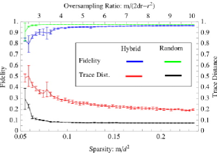
Figure 1: Average fidelity and trace distance vs. (scaled) number of measurement settings $m$ for random states of $n=8$ qubits, so $d=2^{n}$. As discussed in the text, the sampled states had rank $r=3$, depolarizing noise of $5\%$ and Gaussian statistical noise with $\sigma=0.1/d$. Both the random Pauli and hybrid approaches are shown.

Discussion.

We have presented new methods for low-rank quantum state tomography, which require only $O(rd\,\log^{2}(d))$ measurements, where $r$ is the rank of the unknown density matrix and $d$ is the Hilbert space dimension. Our methods are based on and further develop the new paradigm of compressed sensing, and in particular, matrix completion Candes2008 ; Candes2009a . We use measurements that are experimentally feasible, together with very fast classical post-processing. The methods perform well in practice, and are also supported by theoretical guarantees. It would be interesting to further flesh out the trade off between the need for measurements that can be performed easily in an experiment and the need for sparse matrices during the classical post-processing step. It is the hope that this work stimulates such further investigations.

Acknowledgments. We thank E. Candès and Y. Plan for useful discussions. Research at PI is supported by the Government of Canada through Industry Canada and by the Province of Ontario through the Ministry of Research & Innovation. YL is supported by an NSF Mathematical Sciences Postdoctoral Fellowship, JE by the EU (QAP, QESSENCE, MINOS, COMPAS) and the EURYI, DG by the EU (CORNER). We thank the anonymous referees for many helpful suggestions.

I Appendix

I.1 Details of the proof of Theorem 1

While this publication contains a complete proof of all the claims relevant for quantum tomography, the reader is invited to consult the more general and explicit presentation in Ref. prep2 (and soon prep1 ). Below, we provide those details of the proof of Theorem 1, which were left out in the main text.

We introduce some more formal notations used in the argument. Denote the trace inner product between two Hermitian operators $\rho,\sigma$ by $\mbox{$\big{(}\rho,\sigma\big{)}$}:=\operatorname{tr}\rho\sigma$. We assume that $w(A_{1}),\dots,w(A_{m})$ are independent, identically distributed matrix-valued random variables, with $w(A_{i})$ drawn from the $d^{2}$ Pauli matrices with uniform probability. Thus, we model the selection of the observables as a process of sampling with replacement. It is both very plausible and easily provable nesme that drawing the observables without replacement can only yield better results.

I.1.1 Non-commutative large-deviation bound

An essential tool for the proof is a non-commutative large-deviation bound from ahlswede . Let $S=\sum_{i}^{m}X_{i}$ be a sum of i.i.d. matrix-valued random variables (r.v.’s) $X_{i}$. Then it is shown in ahlswede that for every $\lambda,t>0$ we have

$$\Pr[\|S\|>t]\leq 2de^{-\lambda t}\bigl{\|}\mathbbm{E}[e^{\lambda X}]\bigr{\|}^{m}.$$ (7)

It is simple to derive a Bernstein-type inequality from (7). Indeed, assume that $Y$ is some operator-valued random variable with which is bounded in the sense that $\|Y\|\leq 1$ with probability one and which has zero mean $\mathbbm{E}[Y]=0$. Recall the standard estimate

$$1+y\leq e^{y}\leq 1+y+y^{2}$$

valid for real numbers $y\in[-1,1]$ (actually a bit beyond). From the upper bound, we get $e^{Y}\leq\mathbbm{1}+Y+Y^{2}$. From the lower bound:

$$\mathbbm{E}[e^{Y}]\leq\mathbbm{1}+\mathbbm{E}[Y^{2}]\leq\exp(\mathbbm{E}[Y^{2}])$$ (8)

$$\Rightarrow \|\mathbbm{E}[e^{Y}]\|\leq\|\exp(\mathbbm{E}[Y^{2}])\|=\exp(\|\mathbbm{E}[Y^{2}]\|).$$

In order to apply (8) to (7), we set $Y=\lambda X$. The parameter $\lambda$ is chosen to be $\lambda={t}/{(2m\sigma^{2})}$, where $\sigma^{2}=\|\mathbbm{E}[X^{2}]\|$. A straight-forward calculation now gives

$$\Pr[\|S\|>t] \leq 2d\,e^{-t^{2}/4m\sigma^{2}},$$ (9)

(valid for $t\leq 2m\sigma^{2}/\|X\|$).

I.1.2 “Case (i)”: large-deviation bound

The first application of (9) is to verify Eq. (2) from the main text, which claims that

$$\Pr[\|\mathcal{A}-\mathbbm{1}_{T}\|>t]<4dre^{-t^{2}\kappa/8}.$$ (10)

To this end, let $Y_{i}$ be the super-operator defined by

$$Y_{i}(\sigma)=\frac{d^{2}}{m}\mathcal{P}_{T}(w(A_{i}))\,\mbox{$\big{(}w(A_{i}),\mathcal{P}_{T}(\sigma)\big{)}$}.$$

We will employ Eq. (9) on the r.v.’s $X_{i}=(Y_{i}-\mathbbm{E}[Y_{i}])$, where $\mathbbm{E}[Y_{i}]=\frac{1}{m}\mathbbm{1}_{T}$. From the fact that $x\mapsto x^{2}$ is operator convex, one has $\sigma^{2}=\|\mathbbm{E}[(Y-\mathbbm{E}Y)^{2}]\|\leq\|\mathbbm{E}[Y^{2}]\|$. To estimate the latter quantity, we bound (using Hölder’s inequality (c.f. [Bhatia, Matrix Analysis]))

$$\|\mathcal{P}_{T}w_{a}\|_{2}^{2} = \sup_{t\in T,\|t\|_{2}=1}(w_{a},t)^{2}\leq\|w_{a}\|^{2}\|t\|_{\operatorname{tr}}^{2}$$

$$\leq \|w_{a}\|^{2}\,2r\|t\|_{2}^{2}\leq 2\frac{r}{d}.$$

and hence

$$\mathbbm{E}[Y^{2}] = \frac{n^{2}}{m}\mathbbm{E}\big{[}(w_{A},\mathcal{P}_{T}w_{A})\,Y\big{]}$$

$$\leq \frac{d^{2}}{m}\frac{2r}{d}\mathbbm{E}\big{[}Y\big{]}=\frac{2dr}{m^{2}}\,\mathcal{P}_{T}.$$

which implies $\sigma^{2}\leq\frac{2dr}{m^{2}}$. The claimed Eq. (10) directly follows by plugging this estimate of $\sigma^{2}$ into the non-commutative large-deviation bound (9).

I.1.3 “Case (ii)”: the approximate subgradient

Next, consider the claim after Eq. (3) of the main text. There, we assumed that $Y$ was a matrix in $\operatorname{span}(w(A_{1}),\ldots,w(A_{m}))$ such that

$$\|\mathcal{P}_{T}Y-E\|_{2}\leq 1/(2d^{2}),\qquad\|\mathcal{P}_{T}^{\bot}Y\|<1/2.$$ (11)

It is to be shown that $\mathcal{R}\Delta=0$ implies $\|\rho+\Delta\|_{\mathrm{tr}}>\|\rho\|_{\mathrm{\operatorname{tr}}}$.

Recall the scalar sign function $\operatorname{sign}$ which maps positive numbers to $+1$, $0$ to $0$ and negative numbers to $-1$. If $\sigma$ is any Hermitian matrix, then $\operatorname{sign}\sigma$ is the matrix resulting from applying the $\operatorname{sign}$-function to the eigenvalues of $\sigma$. Note that

$$\operatorname{tr}\sigma=(\operatorname{sign}\sigma,\sigma)$$ (12)

and recall Hölder’s inequality bhatia

$$(\sigma_{1},\sigma_{2})\leq\|\sigma_{1}\|_{\mathrm{tr}}\|\sigma_{2}\|$$ (13)

for any two Hermitian $\sigma_{1},\sigma_{2}$.

Letting $F=\operatorname{sign}\Delta_{T}^{\perp}$ we compute:

$$\|\rho+\Delta\|_{\operatorname{tr}} \geq \|E(\rho+\Delta)E\|_{\operatorname{tr}}+\|(\mathbbm{1}-E)(\rho+\Delta)(\mathbbm{1}-E)\|_{\operatorname{tr}}$$

$$\geq (E,\rho+E\Delta E)+\big{(}F,\Delta_{T}^{\bot}\big{)}$$

$$= \|\rho\|_{\operatorname{tr}}+\big{(}E,\Delta_{T}\big{)}+\big{(}F,\Delta_{T}^{\perp}\big{)}-\big{(}Y,\Delta\big{)}$$

$$= \|\rho\|_{\operatorname{tr}}+\big{(}E-\mathcal{P}_{T}Y,\Delta_{T}\big{)}+\big{(}F-\mathcal{P}_{T}^{\bot}Y,\Delta_{T}^{\bot}\big{)}$$

$$> \|\rho\|_{\operatorname{tr}}-\tfrac{1}{2d^{2}}\|\Delta_{T}\|_{2}+\tfrac{1}{2}\|\Delta_{T}^{\bot}\|_{\operatorname{tr}}\geq\|\rho\|_{\operatorname{tr}}.$$

(Use the “pinching inequality” bhatia in the first step; (12), (13) in the second. The third step is (12) and using that $\mathcal{R}\Delta=0$ and $Y\in\operatorname{range}Y$ implies $(Y,\Delta)=0$. The last estimate uses (11) and, once more, (13)).

I.1.4 “Case (ii)”: large deviation bound

The deviation bound before Eq. (5) of the main text follows again from (9). Let $F$ be an arbitrary matrix in $T$. With $X_{i}=\frac{d}{m}\mathcal{P}^{\bot}_{T}(w(A_{i}))\operatorname{tr}w(A_{i})F$:

$$\sigma^{2} = \sup_{\psi,\|\psi\|=1}\frac{1}{d^{2}}\sum_{a}\frac{d^{2}}{m^{2}}\big{(}\operatorname{tr}w_{a}F\big{)}^{2}\langle\psi|(\mathcal{P}_{T}^{\bot}w_{a})^{2}|\psi\rangle$$ (15)

$$\leq \frac{1}{m^{2}}\sum_{a}\big{(}\operatorname{tr}w_{a}F\big{)}^{2}=\frac{d}{m^{2}}\|F\|_{2}^{2},$$

having used that $\|\mathcal{P}_{T}^{\bot}w_{a}\|\leq 1$ and that the $\{d^{-1/2}w_{a}\}$ form an orthonormal basis. Thus

$$\Pr[\|\mathcal{P}^{\bot}_{T}\mathcal{R}F\|>t\|F\|_{2}]<2de^{-t^{2}\kappa r/4}.$$ (16)

In the proof, we use (16) for $t=1/(4\sqrt{r})$. Hence the probability of failure becomes

$$p_{3}\leq 2de^{-\frac{\kappa}{64}}.$$

I.2 Details for Observation 1

In this subsection we need to assume that the Paulis are sampled without replacement. All previous bounds continue to hold — see remark above. Let

$$\mathcal{Q}:\>\rho\mapsto\frac{1}{d}\sum_{i=1}^{m}w(A_{i})\operatorname{Tr}\rho w(A_{i})$$

be the projection operator onto $\operatorname{range}\mathcal{R}$, normalized so that $\lVert\mathcal{Q}\rVert=1$. Define $\gamma=\frac{m}{d^{2}}$, and note that $\mathcal{Q}=\gamma\mathcal{R}$. The optimization program (6) of the main text becomes $\min\|\sigma\|_{\operatorname{tr}}$, s.t. $\|\mathcal{Q}\sigma-\mathcal{Q}\omega\|_{2}\leq\gamma\varepsilon$.

Let $\Delta=\sigma-\rho$. We upper-bound $\lVert\mathcal{Q}{\Delta}\rVert_{2}$ as follows. First,

$$\lVert\mathcal{Q}{\Delta}\rVert_{2}\leq\lVert\mathcal{Q}(\sigma-\omega)\rVert_{2}+\lVert\mathcal{Q}(\omega-\rho_{t})\rVert_{2}+\lVert\mathcal{Q}(\rho_{t}-\rho)\rVert_{2}.$$

For any feasible $\sigma$, the first term is bounded by $\gamma\varepsilon$, while the second term is bounded by $\gamma\varepsilon_{2}$. For the third term, note that for the fixed matrix $\rho_{t}-\rho$, $\mathbbm{E}[\lVert\mathcal{Q}(\rho_{t}-\rho)\rVert_{2}^{2}]=\gamma\lVert\rho_{t}-\rho\rVert_{2}^{2}$, so by Markov’s inequality, $\lVert\mathcal{Q}(\rho_{t}-\rho)\rVert_{2}^{2}\leq\lambda^{2}\gamma\lVert\rho_{t}-\rho\rVert_{2}^{2}$, with probability at least $1-\frac{1}{\lambda^{2}}$ markov . Thus we have

$$\lVert\mathcal{Q}{\Delta}\rVert_{2}\leq\gamma\varepsilon+\gamma\varepsilon_{2}+\lambda\sqrt{\gamma}\varepsilon_{1}\leq 2\gamma\varepsilon=2\delta$$

(where we defined $\delta=\gamma\varepsilon$).

On the other hand, we can also lower-bound $\lVert\mathcal{Q}{\Delta}\rVert_{2}$ as follows: $\|\mathcal{Q}\Delta\|_{2}\geq\|\mathcal{Q}\Delta_{T}\|_{2}-\|\mathcal{Q}\Delta_{T}^{\bot}\|_{2}$. For the second term, we have $\|\mathcal{Q}\Delta_{T}^{\bot}\|_{2}\leq\|\Delta_{T}^{\bot}\|_{2}$ (we cannot use Markov’s inequality, because here we require a bound that holds simultaneously for all $\Delta$). For the first term, recall from the noise-free case that $\mathcal{A}=\mathcal{P}_{T}\mathcal{R}\mathcal{P}_{T}$ satisfies $\|\mathbbm{1}_{T}-\mathcal{A}\|<1/2$ with high probability, and hence we have $\|\mathcal{Q}\Delta_{T}\|_{2}\geq\gamma\|\mathcal{A}\Delta_{T}\|_{2}\geq\tfrac{1}{2}\gamma\|\Delta_{T}\|_{2}$. So we have

$$\|\mathcal{Q}\Delta\|_{2}\geq\tfrac{1}{2}\gamma\|\Delta_{T}\|_{2}-\|\Delta_{T}^{\bot}\|_{2}.$$

Combining the above two inequalities and rearranging, we get

$$\|\Delta_{T}\|_{2}\leq\frac{2}{\gamma}\big{(}2\delta+\|\Delta_{T}^{\bot}\|_{2}\big{)}\leq\frac{2}{\gamma}\big{(}2\delta+\|\Delta_{T}^{\bot}\|_{\operatorname{tr}}\big{)}.$$ (17)

We now show that $\|\rho+\Delta\|_{\operatorname{tr}}<\|\rho\|_{\operatorname{tr}}$ implies that $\Delta$ must be small. With the estimate (17) at our disposal, we re-visit (I.1.3):

$$\|\rho+\Delta\|_{\operatorname{tr}}-\|\rho\|_{\operatorname{tr}}$$

$$\geq \big{(}E,\Delta_{T}\big{)}+\big{(}F,\Delta_{T}^{\perp}\big{)}-\big{(}Y,\Delta\big{)}+\big{(}Y,\Delta\big{)}$$

$$= \big{(}E-\mathcal{P}_{T}(Y),\Delta_{T}\big{)}+\big{(}F-\mathcal{P}_{T}^{\perp}(Y),\Delta_{T}^{\perp}\big{)}+\big{(}Y,\mathcal{Q}(\Delta)\big{)}$$

$$> -\frac{1}{2d^{2}}\|\Delta_{T}\|_{2}+\frac{1}{2}\|\Delta_{T}^{\bot}\|_{\operatorname{tr}}-2\delta\|Y\|_{2}$$

$$\geq -\frac{1}{2d^{2}}\cdot\frac{2}{\gamma}(2\delta+\|\Delta_{T}^{\bot}\|_{\operatorname{tr}})+\frac{1}{2}\|\Delta_{T}^{\bot}\|_{\operatorname{tr}}-2\delta\|Y\|_{2}$$

$$= (\tfrac{1}{2}-\tfrac{1}{m})\lVert\Delta_{T}^{\perp}\rVert_{\operatorname{tr}}-2\delta(\tfrac{1}{m}+\lVert Y\rVert_{2}).$$

We use a crude bound $\lVert Y\rVert_{2}=\lVert\mathcal{P}_{T}(Y)\rVert_{2}+\lVert\mathcal{P}_{T}^{\perp}(Y)\rVert_{2}\leq\lVert\mathcal{P}_{T}(Y)-E\rVert_{2}+\lVert E\rVert_{2}+\lVert\mathcal{P}_{T}^{\perp}(Y)\rVert\sqrt{d}\leq\frac{1}{2d^{2}}+\sqrt{r}+\frac{1}{2}\sqrt{d}$. Then, for reasonable values of the parameters (say $d\geq 16$, $m\geq 16$, $r\leq d/10$), we have

$$\|\rho+\Delta\|_{\operatorname{tr}}-\|\rho\|_{\operatorname{tr}}>\tfrac{7}{16}\lVert\Delta_{T}^{\perp}\rVert_{\operatorname{tr}}-2\delta\sqrt{d}.$$

So $\|\rho+\Delta\|_{\operatorname{tr}}<\|\rho\|_{\operatorname{tr}}$ implies

$$\lVert\Delta_{T}^{\perp}\rVert_{\operatorname{tr}}<\tfrac{32}{7}\delta\sqrt{d}.$$ (18)

Finally, write $\lVert\Delta\rVert_{\operatorname{tr}}\leq\sqrt{2r}\lVert\Delta_{T}\rVert_{2}+\lVert\Delta_{T}^{\perp}\rVert_{\operatorname{tr}}$, and use (17) and (18). After simplifying, substituting in $\delta=\gamma\varepsilon$, and setting $\kappa=m/(rd)$, one obtains

$$\begin{split}\lVert\Delta\rVert_{\operatorname{tr}}&\leq 6\varepsilon\sqrt{r}+13\varepsilon\sqrt{rd}+5\varepsilon\frac{\kappa r}{\sqrt{d}}\leq O(\varepsilon\sqrt{rd}).\end{split}$$ (19)

Finally, we write $\lVert\sigma-\rho_{t}\rVert_{\operatorname{tr}}\leq\lVert\sigma-\rho\rVert_{\operatorname{tr}}+\lVert\rho-\rho_{t}\rVert_{\operatorname{tr}}$. The first term is bounded by $O(\varepsilon\sqrt{rd})$ as shown above; the second term is $\leq\lVert\rho-\rho_{t}\rVert_{2}\sqrt{d}\leq\varepsilon_{1}\sqrt{d}\leq\varepsilon\sqrt{d}$. This gives the desired result.

I.3 Certified tomography for almost-pure states

For almost-pure states ($r=1$), it is possible to obtain estimates for $\delta_{1}$ from only $O(d)$ Pauli expectation values without any assumptions. In this subsection, we sketch a simple scheme based on this observation: it outputs a reconstructed density matrix $\sigma$, together with a certified bound on the deviation $\|\sigma-\rho_{t}\|_{\operatorname{tr}}$. The algorithm takes two inputs: $O(d\,\log^{2}d)$ random Pauli expectation values, and the experimentalist’s estimate of the measurement precision $\delta_{2}$ errormodel .

Concretely, we set $r=1$ and aim to put a bound on $\delta_{1}=\|\rho_{t}-|\psi\rangle\langle\psi|\|_{2}$, where $|\psi\rangle$ is the eigenvector of $\rho_{t}$ corresponding to the largest eigenvalue. Such a bound can be obtained in terms of the purity $\operatorname{tr}\rho_{t}^{2}=\|\rho_{t}\|_{2}^{2}$. E.g.,

$$\delta_{1}=\|\rho_{t}-|\psi\rangle\langle\psi|\|_{2}\leq 2^{1/2}(1-\|\rho_{t}\|_{2}^{2})$$ (20)

(valid for $\|\rho_{t}\|\geq 1/2$, which can certifiably be tested). Estimating the purity is done in a way analogous to the proof of Theorem 1. Choose $m$ i.i.d. random variables $A_{i}$ taking values in $[1,d^{2}]$, and define $S=(d/m)\sum_{i=1}^{m}|\operatorname{tr}w(A_{i})\omega|^{2}$. Then $\mathbbm{E}[S]=\|\omega\|_{2}^{2}$ and thus $\|\rho_{t}\|_{2}\geq\mathbbm{E}[S]^{1/2}-\delta_{2}$. We can bound the deviation of $S$ from its expected value by the standard (commutative) Chernoff bound. One finds for the variance $\operatorname{Var}((d/m)|\operatorname{tr}w(A)\omega|^{2})\leq(d/m^{2})\|\omega\|_{2}^{2}\leq d/m^{2},$ so that (for $t\in[0,1]$):

$$\Pr\bigl{[}\bigl{|}S-\|\omega\|_{2}^{2}\bigr{|}>t\bigr{]} \leq 2e^{-t^{2}m/(4d)},$$

Choose $m=4\mu d/t^{2}$ for some $\mu>1$ to ensure that

$$\Pr[|S-\|\rho_{t}\|^{2}_{2}|>t+2\delta_{2}+\delta_{2}^{2}]<e^{-\mu}.$$ (21)

Combining the previous equation with (20), we have arrived at a certified estimate for $\delta_{1}$.

I.4 A hybrid approach to matrix recovery

Matrix recovery using Pauli measurements does lack one desirable feature: the classical post-processing (solving the convex programs) is more costly, compared to matrix completion Candes2008 ; Candes2009a . This is due to the role of sparse linear algebra in the SVT (singular value thresholding) algorithm Cai2008 . The basic issue is that SVT must handle matrices of the form $\mathcal{R}\rho$. For matrix completion, $\mathcal{R}\rho$ is sparse, so basic operations such as matrix-vector multiplication take time $O(d)$; but when we use random Pauli measurements, $\mathcal{R}(\rho)$ is dense, and basic operations take time $O(d^{2})$. We now describe a “hybrid” approach that avoids this difficulty, and works well in practice. The main observation is that for certain, carefully selected sets of Pauli matrices, $\mathcal{R}\rho$ is sparse after all.

Any Pauli matrix is of the form

$$w(u,v)=\bigotimes_{k=1}^{n}i^{u_{k}v_{k}}(\sigma^{x})^{u_{k}}(\sigma^{z})^{v_{k}}$$

for $u,v\in\{0,1\}^{n}$. Plainly, the position of the $d$ non-zero matrix elements of $w(u,v)$ depends only on $u$ ($v$ encodes only phase information). Now choose a random subset $S\subset\{0,1\}^{n}$ of size $O(r\operatorname{polylog}(d))$, and then for all $u\in S$ and $v\in\{0,1\}^{n}$, measure the Pauli matrix $w(u,v)$. Thus we are measuring each of the Pauli strings containing only $\sigma^{z}$ or identity, together with these same strings “masked” by applying a set of size $|S|$ of Pauli strings with a pattern of $\sigma^{x}$ and identity. Formally, this means

$$\mathcal{R}\rho\propto\sum_{u\in S,v\in\{0,1\}^{n}}w(u,v)\operatorname{tr}(\rho w(u,v)).$$

It follows that $\mathcal{R}\rho$ is sparse with only $|S|d$ non-zero matrix elements. This “hybrid method” can be viewed as a variant of the usual matrix completion problem, where instead of sampling matrix elements independently at random, we sample groups of matrix elements determined by the random strings $u\in S$.

While the hybrid algorithm works well for generic states, certain input states $\rho$ may fail to be “incoherent enough” w.r.t. the very specific set expectation values obtained (c.f. Candes2008 ; Candes2009a ). For example, when the eigenvectors of $\rho$ are nearly aligned with the standard basis, most of the matrix elements of $\rho$ are nearly 0, and hence matrix completion is impossible. To avoid this problem, we suggest to perform a pseudo-random unitary $U$ prior to measuring the Pauli matrices. One then uses the hybrid method on $U\rho U^{\dagger}$, and finally applies $U^{-1}$ to recover $\rho$. In particular, one can draw $U$ at random from an (approximate) unitary $k$-design with $k\sim n/\log n$. Explicit constructions of such unitaries are known, and can be implemented efficiently harrow-low .

While we cannot at this point prove rigorous guarantees for the hybrid approach, we do show below that randomization by approximate $k$-designs generates sufficient “incoherence” that the original matrix completion algorithms Candes2008 ; Candes2009a would work. Because these algorithms call for matrix elements to be sampled from a uniform distribution, Observation 3 does not rigorously apply to the hybrid scheme. It does, however, make it plausible that pseudo-randomization overcomes incoherence problems and that guarantees for the hybrid method can be proven in the future.

Observation 3 (Incoherence from $k$-designs)

Let $\rho$ be an arbitrary state of rank $r$ and dimension $d$, and let $E$ be the projector onto the support of $\rho$. Let $|i\rangle$, $i=1,\ldots,d$, denote the standard basis. Let $U$ be drawn at random from an ($\varepsilon$-approximate) unitary $k$-design with $k\sim n/\log n$ (and $\varepsilon=1/d^{k}$), and let $|b_{i}\rangle=U|i\rangle$. Then, with probability at least $1-(1/d)$, the following holds:

$$\text{for all $i=1,\ldots,d$, }\lVert E|b_{i}\rangle\rVert^{2}_{2}\leq\mu_{0}r/d,$$

where $\mu_{0}=C_{1}(\log d)^{C_{2}}$, and $C_{1}$ and $C_{2}$ are fixed constants.

This implies the incoherence conditions (A0) and (A1) of Candes2008 , specialized to the case of positive semidefinite matrices, with $\mu_{0}$ as given above and $\mu_{1}=\mu_{0}\sqrt{r}$. Combining with the results of Candes2008 shows that ordinary matrix completion, with matrix elements sampled independently at random, will succeed. This guarantee does not extend to the hybrid method, however.

Proof of Observation 3: First consider a single vector $|b_{1}\rangle$, and define $Z=\lVert E|b_{1}\rangle\rVert^{2}_{2}$. We will compute the $k$’th moment of $Z$:

$$\begin{split}\mathbbm{E}[Z^{k}]&=\mathbbm{E}[\operatorname{Tr}(E^{\otimes k}|b_{1}\rangle\langle b_{1}|^{\otimes k}E^{\otimes k})]\\ &=\operatorname{Tr}(E^{\otimes k}\mathbbm{E}[|b_{1}\rangle\langle b_{1}|^{\otimes k}]E^{\otimes k}).\end{split}$$

We want to compute $\mathbbm{E}[|b_{1}\rangle\langle b_{1}|^{\otimes k}]$. Let $|u_{1}\rangle$ be a Haar-random unit vector in $\mathbbm{C}^{d}$, and let

$$\Delta=\mathbbm{E}[|b_{1}\rangle\langle b_{1}|^{\otimes k}]-\mathbbm{E}[|u_{1}\rangle\langle u_{1}|^{\otimes k}].$$

By the definition of an approximate unitary $k$-design, every matrix element of $\Delta$ has absolute value at most $\varepsilon/d^{k}$. Thus $\lVert\Delta\rVert_{2}\leq\varepsilon$. A well-known (c.f. e.g. Def. 2.1 in harrow-low-cmp ) corollary of Schur’s Lemma states $\mathbbm{E}[|u_{1}\rangle\langle u_{1}|^{\otimes k}]=\Pi_{S}/\dim(S)$, where $S$ is the symmetric subspace of $(\mathbbm{C}^{d})^{\otimes k}$, $\Pi_{S}$ is the projector onto $S$, and $\dim(S)=\binom{d+k-1}{k}$. So we have

$$\mathbbm{E}[|b_{1}\rangle\langle b_{1}|^{\otimes k}]=\frac{\Pi_{S}}{\dim(S)}+\Delta.$$

Substituting in, we get:

$$\begin{split}\mathbbm{E}[Z^{k}]&=\frac{\operatorname{Tr}E^{\otimes k}\Pi_{S}}{\dim(S)}+\operatorname{Tr}E^{\otimes k}\Delta\\ &\leq\frac{\lVert E^{\otimes k}\rVert_{\operatorname{tr}}\lVert\Pi_{S}\rVert}{\dim(S)}+\lVert E^{\otimes k}\rVert_{2}\lVert\Delta\rVert_{2}\\ &\leq\frac{r^{k}k!}{(d+k-1)\cdots d}+\varepsilon\sqrt{r^{k}}\leq\Bigl{(}\frac{rk}{d}\Bigr{)}^{k}.\end{split}$$

Using Markov’s inequality, and setting $t=(rk/d)\cdot d^{2/k}\leq(r/d)\cdot\text{poly}(\log d)$, we get

$$\Pr[Z>t]\leq\frac{\mathbbm{E}[Z^{k}]}{t^{k}}\leq\Bigl{(}\frac{rk}{td}\Bigr{)}^{k}=\frac{1}{d^{2}}.$$

This proves the claim for a single vector $|b_{1}\rangle$. Now take the union bound over all the vectors $|b_{i}\rangle$, $i=1,\ldots,d$. $\square$

References

(1)Quantum state estimation, No. 649 in Lect. Notes Phys., M. Paris
and J. Řeháček, eds., (Springer, Heidelberg, 2004).
(2)
H. Häffner et al., Nature 438, 643 (2005).
(3)
J. L. O’Brien et al., Nature 426, 264 (2003).
(4)
M. S. Kaznady and D. F. V. James, Phys. Rev. A 79, 022109 (2009).
(5)
G. M. D’Ariano, L. Maccone, and M. Paini,
J. Opt. B 5, 77 (2003); V. V. Dodonov and V. I. Man’ko, Phys. Lett. A 229, 335 (1997).
(6) J.-P. Amiet and S. Weigert, J. Phys. A 32, 2777 (1999).
(7)
B. K. Natarajan, SIAM J. Comp. 24, 227 (1995).
(8)
D. Donoho, IEEE Trans. Info. Theory 52, 1289 (2006);
E. Candès and
T. Tao, IEEE Trans. Info. Theory 52, 5406 (2006).
(9)
R. L. Kosut, arXiv:0812.4323.
(10)
E. J. Candès and B. Recht, Found. Comp. Math. 9, 717 (2008).
(11) E. J. Candès and T. Tao, IEEE Trans. Inform. Th., arXiv:0903.1476.
(12)
E. J. Candès and Y. Plan, Proc. IEEE, in press (2010), arXiv:0903.3131.
(13)
M. Fazel, E. Candès, B. Recht and P. Parrilo,
Proc. Asilomar Conf. CA, Nov 2008.
(14)
J.-F. Cai, E. J. Candès, and Z. Shen, arXiv:0810.3286.
(15)
A. W. Harrow and R. A. Low, Proc. Random 2009, LNCS 5687, 548 (2009);
D. Gross, K. Audenaert, and J. Eisert, J. Math. Phys. 48,
052104 (2007).
(16)
The techniques easily generalize to spin- particles prep2 .
(17) We use the usual matrix norms , with the singular values of . The last
definition extends to super-operators: if is a
super-operator, then is its largest singular value,
or, equivalently (a.k.a. “”-norm).
(18)
If the term were zero, would be a
strict subgradient.
(19)
Going beyond
Candes2009 , we bound deviations in -norm, as opposed to
-norm. The former norm gives stronger results and carries an
operational meaning in terms of statistical distinguishability.
(20)
Consider a pure state of qubits subject to local noise that occurs with probability on each site. Then the density matrix is well-approximated by a matrix of rank ,
where is the binary entropy of , and is the Hilbert space dimension. When is small, we have .
(21)
The bounds presented here hold even for a worst-case scenario of
“adversarial” noise. Employing more realistic noise
models (e.g., independent Gaussian errors for each Pauli expectation
value) gives rise to significantly improved estimates prep1 .
(22)
R. Ahlswede and A. Winter,
IEEE Trans. Inf. Theory 48, 569 (2002).
(23)
R. Bhatia,
Matrix analysis (Springer, Berlin, 1997).
(24)
S. Becker, S. T. Flammia, D. Gross, Y.-K. Liu, and J. Eisert, in preparation.
(25)
D. Gross, arxiv:0910.1879.
(26)
The estimate returned by SVT typically has a subnormalized trace, which we
handle in an ad hoc way by renormalizing. A more accurate estimate
can be obtained by debiasing, or by solving a reformulation of the problem in terms of
-regularized least squares prep1 .
(27)
D. Gross and V. Nesme, arxiv:1001.2738 (2010).
(28)
A. W. Harrow and R. A. Low,
Comm. Math. Phys., 291, 257 (2009).
(29)
Using Theorem 11 of prep2 , the Markov bound can immediately
be replace by a more sophisticated large deviation bound, which
gives a probability of failure exponentially small in .